
Azimuthal Variation in the Surface-Wave Velocity in the Arabian Plate
Higher Polytechnic School, University of Almeria, 04120 Almeria, Spain
Appl. Sci. 2024, 14(12), 5142; https://doi.org/10.3390/app14125142
Submission received: 29 April 2024
/
Revised: 23 May 2024
/
Accepted: 12 June 2024
/
Published: 13 June 2024
(This article belongs to the Special Issue Advances in Geosciences: Techniques, Applications, and Challenges)
Abstract
:This pioneer study determined the azimuthal variation in surface-wave fundamental-mode phase velocity for the Arabian plate, concluding that this variation is not due to seismic anisotropy but to lateral heterogeneity, which is compatible with anisotropic earth models of azimuthal isotropy. The study area was divided in six regions with similar surface-wave phase velocities. We determined their corresponding SH and SV-velocity models versus depth (from 0 to 260 km) by means of the anisotropic inversion of surface-wave phase velocities under the hypothesis of surface-wave propagation in slightly anisotropic media. We observed seismic anisotropy from 10 to 100 km depth. From these models, the parameter ξ was calculated for each region, and the most conspicuous features of the study area were described in terms of this parameter, such as the existence of the plume material propagation in the Arabian shield from the Afar plume, or the existence of a lithospheric keel, which was observed in previous studies beneath the Arabian platform, the Mesopotamian Plain and the Zagros belt.
1. Introduction
Seismic anisotropy can provide direct and independent information on geodynamics through the directional changes in seismic velocities, which can be related to the mantle flow and/or deformation (e.g., [1,2]). This information is particularly interesting for the Arabian plate, because its geodynamics are very complex due to the extensional/compressional regimes that exist around this plate [3]. Shear-wave splitting can be used to estimate anisotropy (e.g., [4]), but this technique provides limited constraints on the depth distribution of the anisotropy. This limitation is overcome if the velocity of the shear waves polarized vertically (βV) and horizontally (βH) is calculated versus depth, i.e., determining S-velocity distributions (βV, βH) with depth, such as those derived from surface-wave analysis. Thus, the goals of the present study are the determination of the azimuthal variation in surface-wave fundamental-mode phase velocity for the Arabian plate, and the parameter ξ = (βH/βV)2 versus depth, from the Love- and Rayleigh-wave dispersion curves anisotropically inverted ([5,6]).
2. Data, Methodology and Results
The traces of 109 earthquakes (Supplement 1), registered by the station: RAYN (Supplement 2), have been analyzed to calculate the fundamental-mode surface-wave group velocities. The earthquakes’ epicenters have been grouped into 56 source zones (Supplement 3), as described by Corchete et al. [7]. These source zones are defined as a location in which seismic events with similar epicenter coordinates have occurred, i.e., seismic events with a coordinate difference less than or equal to 0.5 degrees in latitude and longitude. Thus, a path coverage of the study area of 56 source-station paths of surface-wave group velocities is determined (Figure 1a). Figure 1b,c show that the number of paths of Love waves decreases more rapidly than that corresponding to the Rayleigh waves. The group velocities corresponding to these paths have been determined by means of a combination of the Multiple Filter Technique (MFT; [8]) and the Time Variable Filtering (TVF; [9]), as described by Corchete et al. [7]. Figure 2 and Figure 3 show examples of the group-velocity calculation for the Love and Rayleigh waves, respectively. However, the methodology used to determine the seismic anisotropy [5], in the present study, considers phase velocities as observed data. Then, the phase velocities must be determined from their corresponding group velocities. This computation is performed as described by Corchete [6], and Figure 4 shows an example of the phase velocity computation for the group velocities shown in Figure 2c and Figure 3c (magenta line). Figure 5 shows the Love and Rayleigh phase velocities (dispersion curves) determined for the events involved in the path S23-RAYN (Supplements 2, 3 and Figure 1a), and this method is followed to calculate the dispersion curves for all paths shown in Figure 1a, and these curves are fitted to the formula [5].
where c is the phase velocity, ω = 2π/T, T is the period and θ is the azimuth of the wave-number vector. Formula (1) expresses the azimuthal variation in Love and Rayleigh phase velocities through a set coefficients Ai (with i varying from 1 to 5) for each type of wave: Love or Rayleigh. Figure 6 shows this azimuthal variation for the periods: 20, 40, 60 and 80 s; and Figure 7 shows the values of the coefficients Ai with the period T. Figure 8a shows the error ε determined between the phase velocity cth given by Equation (1) and the phase velocities cob (the dispersion curves) determined for the paths shown in Figure 1a. This error ε is calculated by
where Ν is the number of paths for each period T (Figure 1b,c) and for each type of wave (Love or Rayleigh). The error ε reaches a minimum value at ~40 s for Love and Rayleigh waves (Figure 8a), and from this value, it remains approximately constant with the period for Rayleigh waves (Figure 8a, blue line), while it increases with the period for Love waves (Figure 8a, red line), because the number of paths of Love waves (Figure 1b) decreases drastically with the period from ~40 s. A new fit of the dispersion curves using Equation (1) is calculated considering only three coefficients Ai (i varying from 1 to 3). Figure 8a (dashed lines) shows that the error ε is greater than that corresponding to the former fit, i.e., the fitting given by Equation (1) with five coefficients is better than that with three coefficients (Figure 8b). Nevertheless, Figure 6 shows that the azimuthal variation in phase velocities is not due to anisotropy but to lateral heterogeneity (Figure 9a; [10]), because Equation (1) does not fit the phase velocities satisfactorily within their errors in general. The best fit of Equation (1) is achieved at the period of 40 s when the coefficients Ai (with i varying from 2 to 5) are in general negligible within their error (Figure 7 and Figure 8a), and the error ε is greater for the period range in which those are not negligible within their error (e.g., 5–40 s; Figure 7 and Figure 8a). This lateral heterogeneity is compatible with anisotropic models of azimuthal isotropy (i.e., hexagonal symmetry or transversely isotropic [11]), which can be calculated if the study area is divided into regions (Figure 1a and Figure 9b). These regions are established considering the areas with similar Rayleigh-wave phase velocities. The Love-wave phase velocities are not considered because they show bigger scatter than the Rayleigh-wave ones (Figure 7 and Figure 8a). In Figure 10b, the Love (black circles) and Rayleigh (black triangles) phase velocities corresponding to the region 1 are shown. They are calculated with the mean of the values determined for each period for the paths plotted in the upper central part of Figure 10 and the small vertical bars present for the Rayleigh-wave values (Figure 10b), which confirms that the dispersion curves considered for this region have similar values. Then, for each region, an isotropic model is defined to calculate the anisotropic model as a small perturbation of this isotropic model ([5,6]). For region 1 (Figure 9b), Table 1 shows this isotropic model, which is calculated from the isotropic inversion of the Rayleigh-wave dispersion, which is determined for the paths that are within this region (Figure 10b [7]). The S-velocity of this model (Figure 10a) is plotted only for depths above 260 km due to the poor resolution obtained for greater depths in this inversion process (Figure 10c). The Rayleigh-wave dispersion is properly fitted by this model, but the Love-wave dispersion is not fitted (Figure 10b), i.e., the Love- and Rayleigh-wave dispersions are not compatible with a unique isotropic model. This Love–Rayleigh discrepancy makes it necessary to consider the existence of seismic anisotropy. This anisotropy is considered with hexagonal symmetry [11], in the depth range from 10 to 100 km (Figure 11a [5,6]), to fit satisfactorily both dispersion curves (Figure 11b). For the other regions (Figure 9b), the same process is followed, selecting an isotropic model for each region (Supplements T1, T2, T3, T4 and T5) and calculating its perturbation in terms of S-velocities (Supplements F1, F2, F3, F4 and F5). Table 2 shows the values of the parameter ξε resulting from the S-velocities determined for each region of Figure 9b.
c(ω, θ) = A1(ω) + A2(ω) cos 2θ + A3(ω) sin 2θ + A4(ω) cos 4θ + A5(ω) sin 4θ
3. Interpretation and Discussion
Depth range: 10–30 km (crust). The parameter ξ (Table 2) shows higher values for the regions 3, 4 and 5. For the region 3 and 4, the higher values of ξ agree with the anisotropic perturbation determined for the Mesopotamian Plain by Kim et al. [3]. These higher values of ξ can be related to the lithospheric keel observed beneath the Mesopotamian Plain ([12,13,14]) and can be also related to the vertical alignment of minerals in the crust due to its horizontal shortening [3], caused by the collision between the Arabian and Eurasian plates from ~14 Ma, which has originated a horizontal lithospheric shortening of the Arabian platform, the Mesopotamian Plain and the Zagros belt. For region 5, the higher values of ξ can be related to shape-induced anisotropy, which is caused by small-scale isotropic heterogeneities preferentially oriented in a strain field [11], as can occur in folded zones such as the Oman-folded zone (OFZ, Figure 9a). This shape-induced anisotropy can exist for the crust and the subcrustal lithosphere. This kind of anisotropy is obviously difficult to interpret, because it is related to a complex geodynamic development, and the resultant pattern of deformations is also very complex.
Depth range: 30–100 km (upper mantle). The parameter ξ (Table 2) shows higher values for the regions 1 (30–100 km-depth), 2 (55–100 km-depth) and 5 (30–100 km-depth). For region 1, the higher values of ξ can be related to the plume material propagation in the Arabian shield, from the Afar plume ([14,15,16,17,18,19,20,21]), and to the Yemeni Oligocene Trapps, which was formed by the infiltration of Afar plume material ~30 Ma [22], and it may indicate the existence of magmatic underplating at crustal depths [23]. Also, these higher values of ξ can be related to the post-12 Ma volcanism in western Arabia [17]. For region 2, the higher values of ξ can be related to mantle plume material from the Jordan plume. Chang and van der Lee [17] determined a low-velocity anomaly in their model just beneath Jordan and northern Arabia, and they related this anomaly to the Jordan plume, suggesting that this plume may have formed the Syrian volcanic rocks. Also, these higher values of ξ can be related to the existence of a lithospheric keel, which was observed beneath the Arabian platform and the Taurus-Zagros folded zone (TZFZ) in previous studies ([12,13,14]). The fast axes directions of the shear-wave splitting data determined for this region in previous studies ([4,24,25,26,27,28]) are interpreted as toroidal flow around a lithospheric keel beneath this region by Kaviani et al. [27].
4. Conclusions
A study similar to the present study may be performed, for any plate, to determine whether the azimuthal variation in surface-wave velocities can be due to seismic anisotropy or to lateral heterogeneity. In the present study, this azimuthal variation is not due to seismic anisotropy but to lateral heterogeneity, which is compatible with anisotropic earth models of hexagonal symmetry (six models of SH and SV-velocity versus depth, from 0 to 260 km). From these models, the parameter ξ is calculated for each region, observing seismic anisotropy only from 10 to 100 km depth, and the following conclusions are obtained from the values determined for ξ:
Depth range: 0–30 km. For regions 3 and 4, the higher values of ξ can be related to the lithospheric keel that exists beneath the Mesopotamian Plain and to the vertical alignment of minerals in the crust due to its horizontal shortening, which is caused by the collision between the Arabian and Eurasian plates from ~14 Ma. For region 5, the higher values of ξ can be related to the shape-induced anisotropy that can occur in the Oman folded zone. This shape-induced anisotropy can exist for the crust and the subcrustal lithosphere.
Depth range: 30–100 km. For region 1, the higher values of ξ can be related to the plume material propagation in the Arabian shield from the Afar plume and to the Yemeni Oligocene Trapps. Also, these higher values of ξ can be related to the post-12 Ma volcanism in western Arabia. For region 2, the higher values of ξ can be related to mantle plume material from the Jordan plume. Also, these higher values of ξ can be related to the existence of a lithospheric keel observed beneath the Arabian platform and the Taurus–Zagros folded zone (TZFZ) in previous studies.
Supplementary Materials
The following supporting information can be downloaded at https://www.mdpi.com/article/10.3390/app14125142/s1.
Funding
This research received no external funding.
Institutional Review Board Statement
Not applicable.
Informed Consent Statement
Not applicable.
Data Availability Statement
Datasets for this research are available in the National Geophysical Data Center (from the web server at https://maps.ngdc.noaa.gov/viewers/grid-extract/index.html (accessed on 12 June 2024)) and in the Incorporated Research Institutions for Seismology (from the web server at http://www.iris.washington.edu/wilber3/find_event (accessed on 12 June 2024)).
Acknowledgments
The National Geophysical Data Center (NGDC) and the Incorporated Research Institutions for Seismology (IRIS), have provided the elevation and seismic data, respectively.
Conflicts of Interest
The author declares no conflict of interest.
References
- Al-Lazki, A.; Ebinger, C.; Kendall, K.; Helffrich, G.; Leroy, S.; Tiberi, C.; Stuart, G.; Al-Toobi, K. Upper mantle anisotropy of southeast Arabia passive margin [Gulf of Aden northern conjugate margin], Oman. Arab. J. Geosci. 2012, 5, 925–934. [Google Scholar] [CrossRef]
- Elsheikh, A.A. Seismic anisotropy and mantle flow beneath East Africa and Arabia. J. Afr. Earth Sci. 2019, 149, 97–108. [Google Scholar] [CrossRef]
- Kim, R.; Witek, M.; Chang, S.-J.; Lim, J.-A.; Mai, P.M.; Zahran, H. Isotropic and radially anisotropic S-velocity structure beneath the Arabian plate inferred from surface wave tomography. Tectonophysics 2023, 862, 229968. [Google Scholar] [CrossRef]
- Qaysi, S.; Liu, K.H.; Gao, S.S. A database of shear-wave splitting measurements for the Arabian Plate. Seismol. Res. Lett. 2018, 89, 2294–2298. [Google Scholar] [CrossRef]
- Corchete, V. Review of the methodology for the inversion of surface-wave phase velocities in a slightly anisotropic medium. Comput. Geosci. 2012, 41, 56–63. [Google Scholar] [CrossRef]
- Corchete, V. Crust and upper mantle structure of Mars determined from surface-wave analysis. Acta Astronaut. 2024. submitted. [Google Scholar]
- Corchete, V.; Chourak, M.; Hussein, H.M. Shear wave velocity structure of the Sinai Peninsula from Rayleigh wave analysis. Surv. Geophys. 2007, 28, 299–324. [Google Scholar] [CrossRef]
- Dziewonski, A.; Bloch, S.; Landisman, M. A technique for the analysis of transient seismic signals. Bull. Seismol. Soc. Am. 1969, 59, 427–444. [Google Scholar] [CrossRef]
- Cara, M. Filtering dispersed wavetrains. Geophys. J. R. Astron. Soc. 1973, 33, 65–80. [Google Scholar] [CrossRef]
- Corchete, V. The first 3D S-velocity model for the lithosphere-asthenosphere system of the Arabian Peninsula and the Iranian plateau. J. Seismol. 2024. submitted. [Google Scholar]
- Babuska, V.; Cara, M. Seismic Anisotropy in the Earth; Kluwer Academic: Dordrecht, The Netherlands, 1991. [Google Scholar]
- Priestley, K.; McKenzie, D.; Barron, J.; Tatar, M.; Debayle, E. The Zagros core: Deformation of the continental lithospheric mantle. Geochem. Geophys. Geosyst. 2012, 13, Q11014. [Google Scholar] [CrossRef]
- Pasyanos, M.E.; Masters, T.G.; Laske, G.; Ma, Z. LITHO1.0: An updated crust and lithospheric model of the Earth. J. Geophys. Res. Solid Earth 2014, 119, 2153–2173. [Google Scholar] [CrossRef]
- Kaviani, A.; Paul, A.; Moradi, A.; Mai, P.M.; Pilia, S.; Boschi, L.; Rümpker, G.; Li, Y.; Tang, Z.; Sandvol, E. Crustal and uppermost mantle shear wave velocity structure beneath the Middle East from surface wave tomography. Geophys. J. Int. 2020, 221, 1349–1365. [Google Scholar] [CrossRef]
- Park, Y.; Nyblade, A.A.; Rodgers, A.J.; Al-Amri, A. S wave velocity structure of the Arabian Shield upper mantle from Rayleigh wave tomography. Geochem. Geophys. Geosyst. 2008, 9, Q07020. [Google Scholar] [CrossRef]
- Krienitz, M.-S.; Haase, K.M.; Mezger, K.; van den Bogaard, P.; Thiemann, V.; Shaikh-Mashail, M.A. Tectonic events, continental intraplate volcanism, and mantle plume activity in northern Arabia: Constraints from geochemistry and Ar-Ar dating of Syrian lavas. Geochem. Geophys. Geosyst. 2009, 10, Q04008. [Google Scholar] [CrossRef]
- Chang, S.-J.; van der Lee, S. Mantle plumes and associated flow beneath Arabia and East Africa. Earth Planet. Sci. Lett. 2011, 302, 448–454. [Google Scholar] [CrossRef]
- Chang, S.-J.; Merino, M.; van Der Lee, S.; Stein, S.; Stein, C.A. Mantle flow beneath Arabia offset from the opening Red Sea. Geophys. Res. Lett. 2011, 38, L04301. [Google Scholar] [CrossRef]
- Yao, Z.; Mooney, W.D.; Zahran, H.M.; Youssef, S.E.H. Upper mantle velocity structure beneath the Arabian shield from Rayleigh surface wave tomography and its implications. J. Geophys. Res. Solid Earth 2017, 122, 6552–6568. [Google Scholar] [CrossRef]
- Tang, Z.; Mai, P.M.; Chang, S.-J.; Zahran, H. Evidence for crustal low shear-wave speed in western Saudi Arabia from multi-scale fundamental-mode Rayleigh-wave group-velocity tomography. Earth Planet. Sci. Lett. 2018, 495, 24–37. [Google Scholar] [CrossRef]
- Lim, J.-A.; Chang, S.-J.; Mai, P.M.; Zahran, H. Asthenospheric flow of plume material beneath Arabia inferred from S wave travel time tomography. J. Geophys. Res. Solid Earth 2020, 125, e2020JB019668. [Google Scholar] [CrossRef]
- Bosworth, W.; Huchon, P.; Mcclay, K. The Red Sea and Gulf of Aden Basins. J. Afr. Earth Sci. 2005, 43, 334–378. [Google Scholar] [CrossRef]
- Korostelev, F.; Basuyau, C.; Leroy, S.; Tiberi, C.; Ahmed, A.; Stuart, G.W.; Keir, D.; Rolandone, F.; Al Ganad, I.; Khanbari, K.; et al. Crustal and upper mantle structure beneath south-western margin of the Arabian Peninsula from teleseismic tomography. Geochem. Geophys. Geosyst. 2014, 15, 2850–2864. [Google Scholar] [CrossRef]
- Gashawbeza, E.M.; Klemperer, S.L.; Nyblade, A.A.; Walker, K.T.; Keranen, K.M. Shear-wave splitting in Ethiopia: Precambrian mantle anisotropy locally modified by Neogene rifting. Geophys. Res. Lett. 2004, 31, L18602. [Google Scholar] [CrossRef]
- Hansen, S.; Schwartz, S.; Al-Amri, A.; Rodgers, A. Combined plate motion and density-driven flow in the asthenosphere beneath Saudi Arabia: Evidence from shear-wave splitting and seismic anisotropy. Geology 2006, 34, 869–872. [Google Scholar] [CrossRef]
- Sadeghi-Bagherabadi, A.; Sobouti, F.; Ghods, A.; Motaghi, K.; Talebian, M.; Chen, L.; Jiang, M.; Ai, Y.; He, Y. Upper mantle anisotropy and deformation beneath the major thrust-and-fold belts of Zagros and Alborz and the Iranian Plateau. Geophys. J. Int. 2018, 214, 1913–1918. [Google Scholar] [CrossRef]
- Kaviani, A.; Mahmoodabadi, M.; Rumpker, G.; Pilia, S.; Tatar, M.; Nilfouroushan, F.; Yamini-Fard, F.; Moradi, A.; Ali, M.Y. Mantle-flow diversion beneath the Iranian plateau induced by Zagros’ lithospheric keel. Sci. Rep. 2021, 11, 2848. [Google Scholar] [CrossRef] [PubMed]
- Pilia, S.; Kaviani, A.; Searle, M.P.; Arroucau, P.; Ali, M.Y.; Watts, A.B. Crustal and mantle deformation inherited from obduction of the Semail ophiloite (Oman) and continental collision (Zagros). Tectonics 2021, 40, e2020TC006644. [Google Scholar] [CrossRef]
Figure 1.
(a) Path coverage of the surface waves for the 56 source-station paths (Supplements 2 and 3). Number of paths calculated for each dispersion-data period determined for Love (b) and Rayleigh (c) waves.
Figure 1.
(a) Path coverage of the surface waves for the 56 source-station paths (Supplements 2 and 3). Number of paths calculated for each dispersion-data period determined for Love (b) and Rayleigh (c) waves.
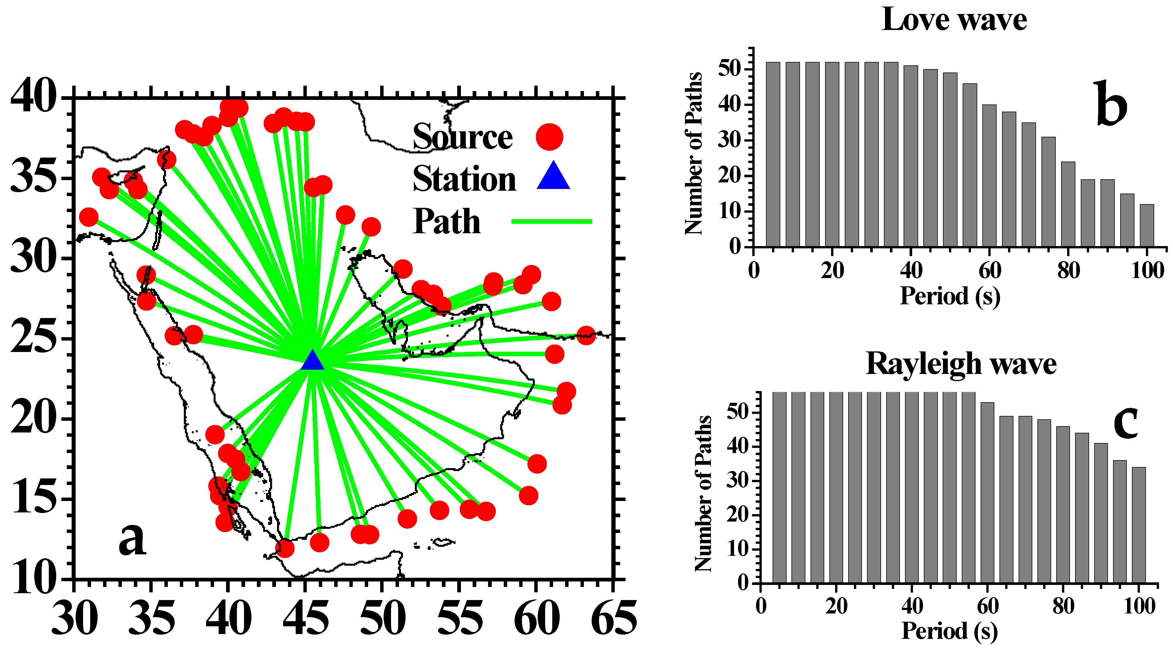
Figure 2.
Love-wave group velocity determination: (a) the observed seismogram (red line) corresponding to the event 70 (Supplement 1) recorded at station: RAYN (Supplement 2, transverse component), instrument corrected. The time-variable filtered seismogram (blue line) calculated from the observed seismogram (red line) and the initial group velocity (b,c). (b) Contour map of relative energy (normalized to 99 decibels) as a function of the period and the group time, calculated from the observed seismogram ((a), red line) with the MFT. The red points denote the group times inferred from the energy map. (c) The initial (red points, (b)) and the final (magenta line, (d)) group velocities calculated from the group times and the epicentral distance. (d) Contour map of relative energy calculated from the time-variable filtered seismogram ((a), blue line) with the MFT. The color scale is the same as in (b).
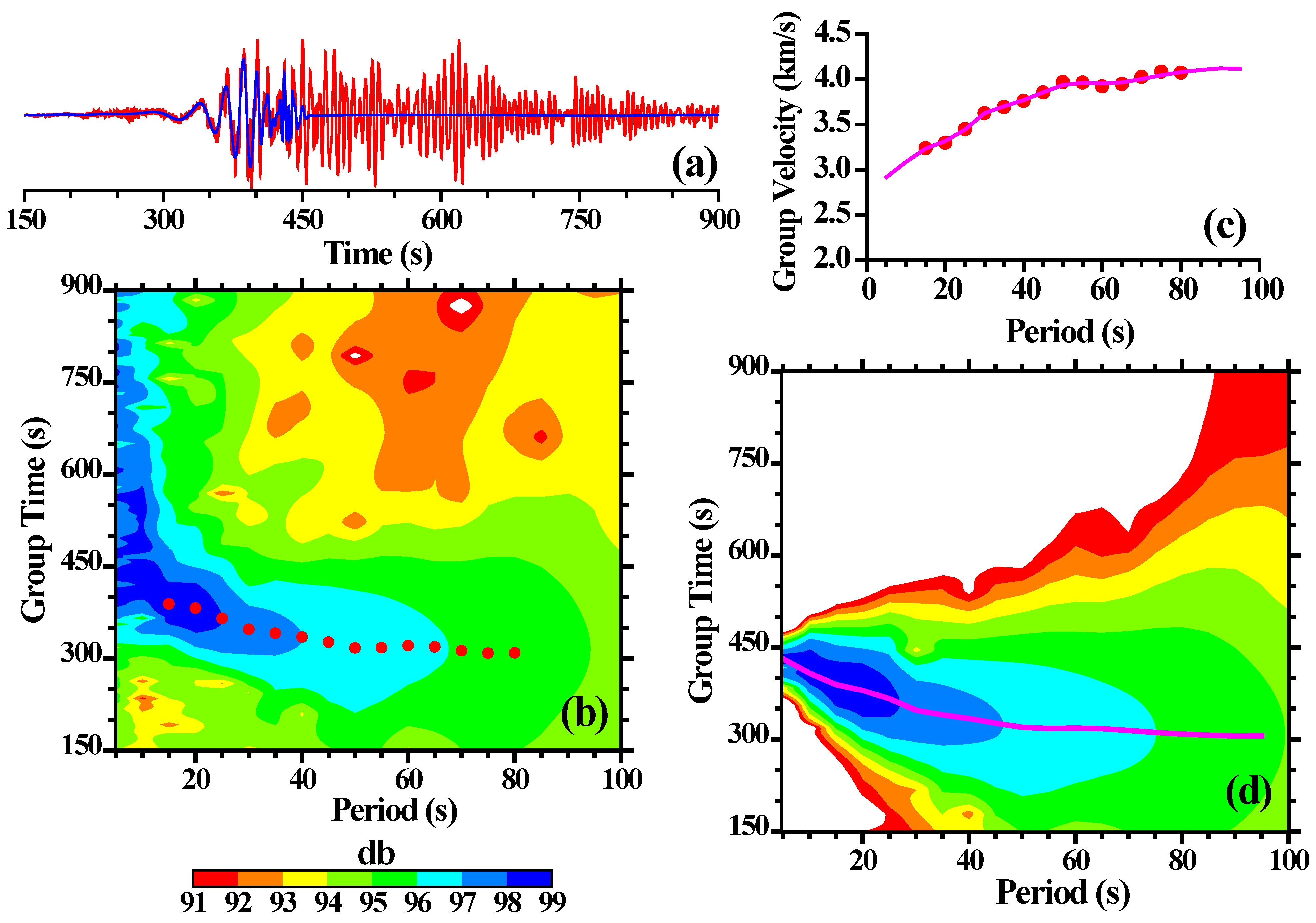
Figure 3.
Rayleigh-wave group velocity determination: (a) the observed seismogram (red line) corresponding to the event 70 (Supplement 1) recorded at station: RAYN (Supplement 2, vertical component), instrument corrected. The time-variable filtered seismogram (blue line) calculated from the observed seismogram (red line) and the initial group velocity (b,c). (b) Contour map of relative energy (normalized to 99 decibels) as a function of the period and the group time calculated from the observed seismogram ((a), red line) with the MFT. The red points denote the group times inferred from the energy map. (c) The initial (red points, (b)) and the final (magenta line, (d)) group velocities calculated from the group times and the epicentral distance. (d) Contour map of relative energy calculated from the time-variable filtered seismogram ((a), blue line) with the MFT. The color scale is the same as in (b).
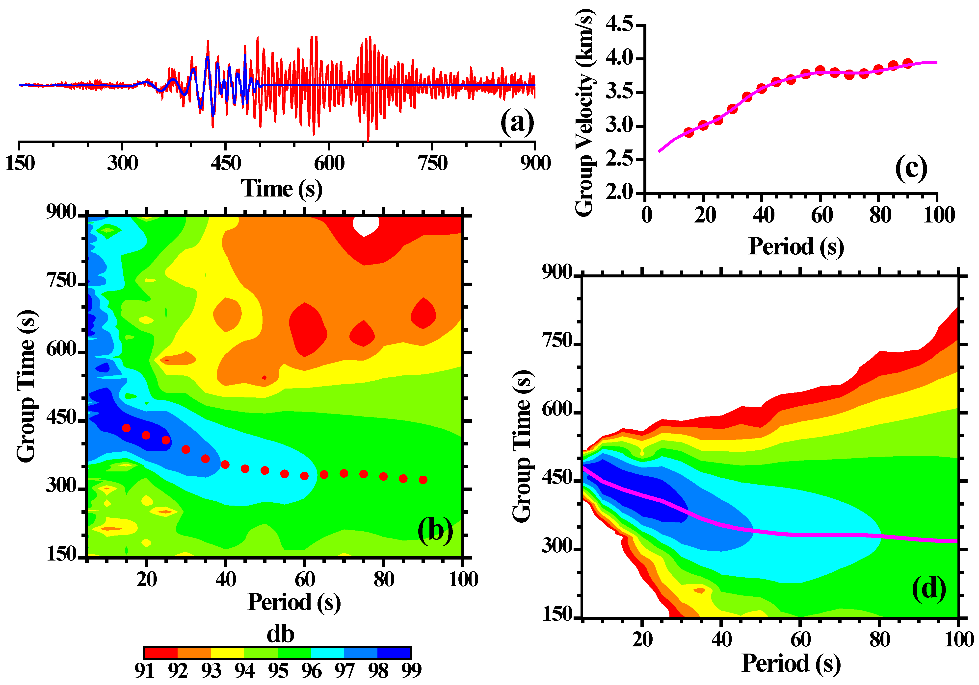
Figure 4.
Love and Rayleigh group velocities (blue line) determined for the traces of the event 70 (Figure 2c and Figure 3c, magenta line), and their corresponding phase velocities (red line) determined from their respective group velocities by inversion.
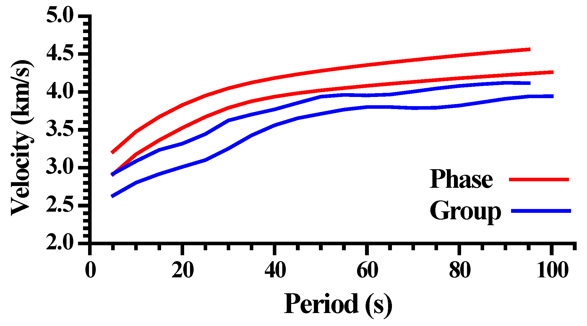
Figure 5.
Love and Rayleigh phase velocities determined for the events involved in the path S23-RAYN (Supplements 2, 3 and Figure 1). The small black circles show the mean of these velocities for each period, and the black vertical bars show the standard deviation.
Figure 5.
Love and Rayleigh phase velocities determined for the events involved in the path S23-RAYN (Supplements 2, 3 and Figure 1). The small black circles show the mean of these velocities for each period, and the black vertical bars show the standard deviation.
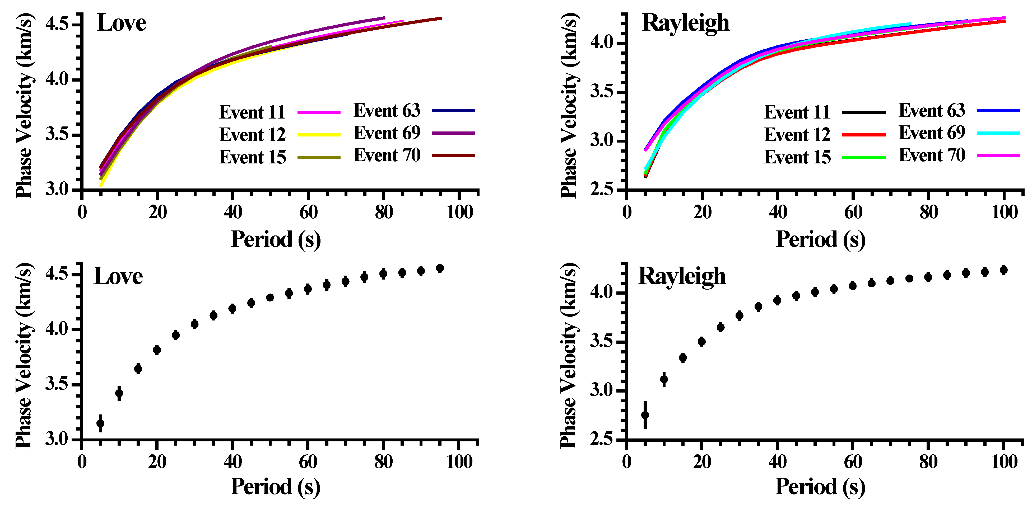
Figure 6.
Azimuthal variation in Love and Rayleigh phase velocities for the periods: 20, 40, 60 and 80 s. The black line shows the phase velocity determined by Formula (1) with the coefficients shown in Figure 7 for each selected period. The small black circles denote Love waves, and the small black triangles denote Rayleigh waves. The black vertical bars denote the standard deviation in phase velocity.
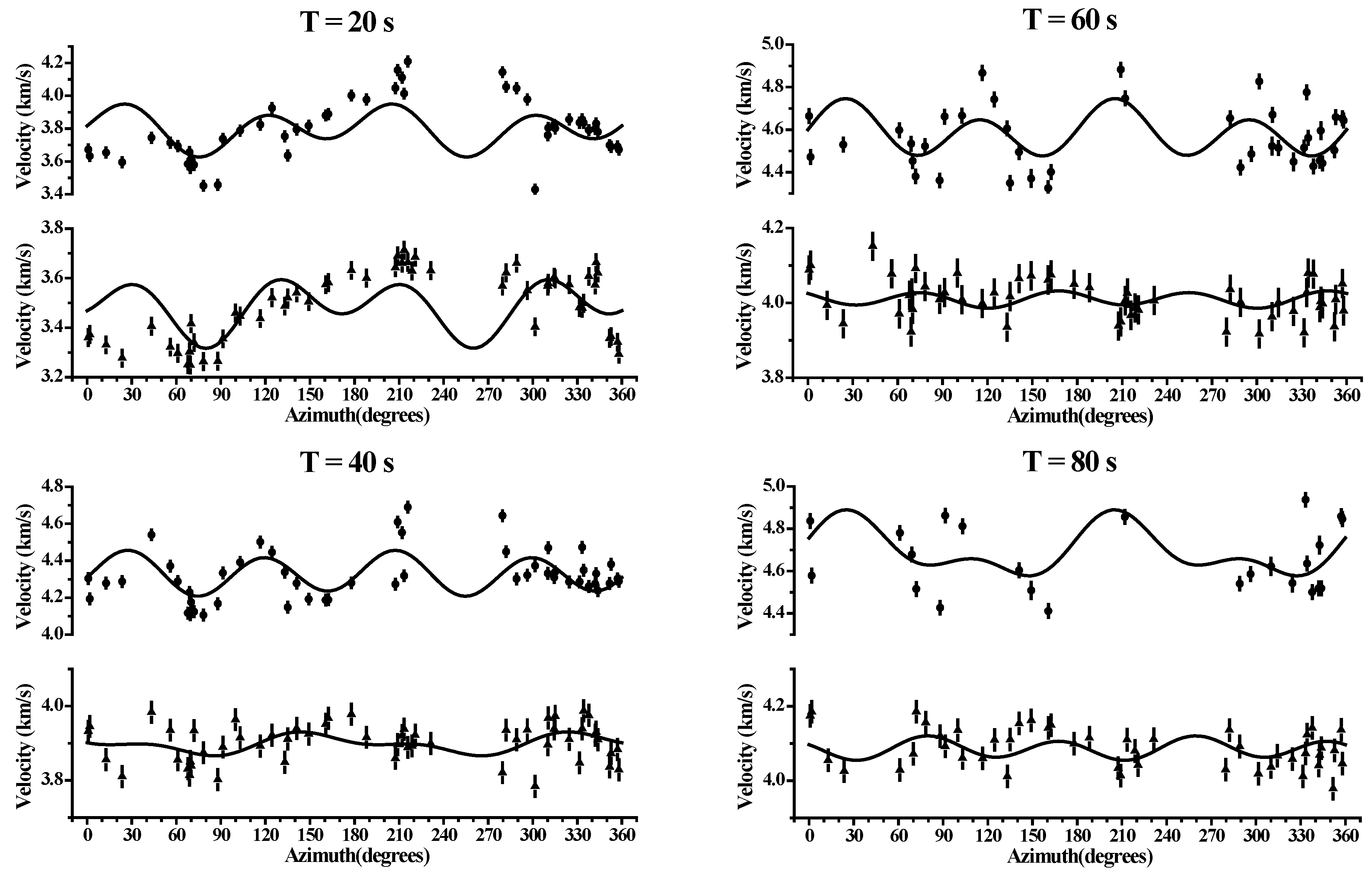
Figure 7.
Ai coefficients of Formula (1). The small black circles denote Love waves, and the small black triangles denote Rayleigh waves. The black vertical bars denote the standard deviation in these coefficients.
Figure 7.
Ai coefficients of Formula (1). The small black circles denote Love waves, and the small black triangles denote Rayleigh waves. The black vertical bars denote the standard deviation in these coefficients.
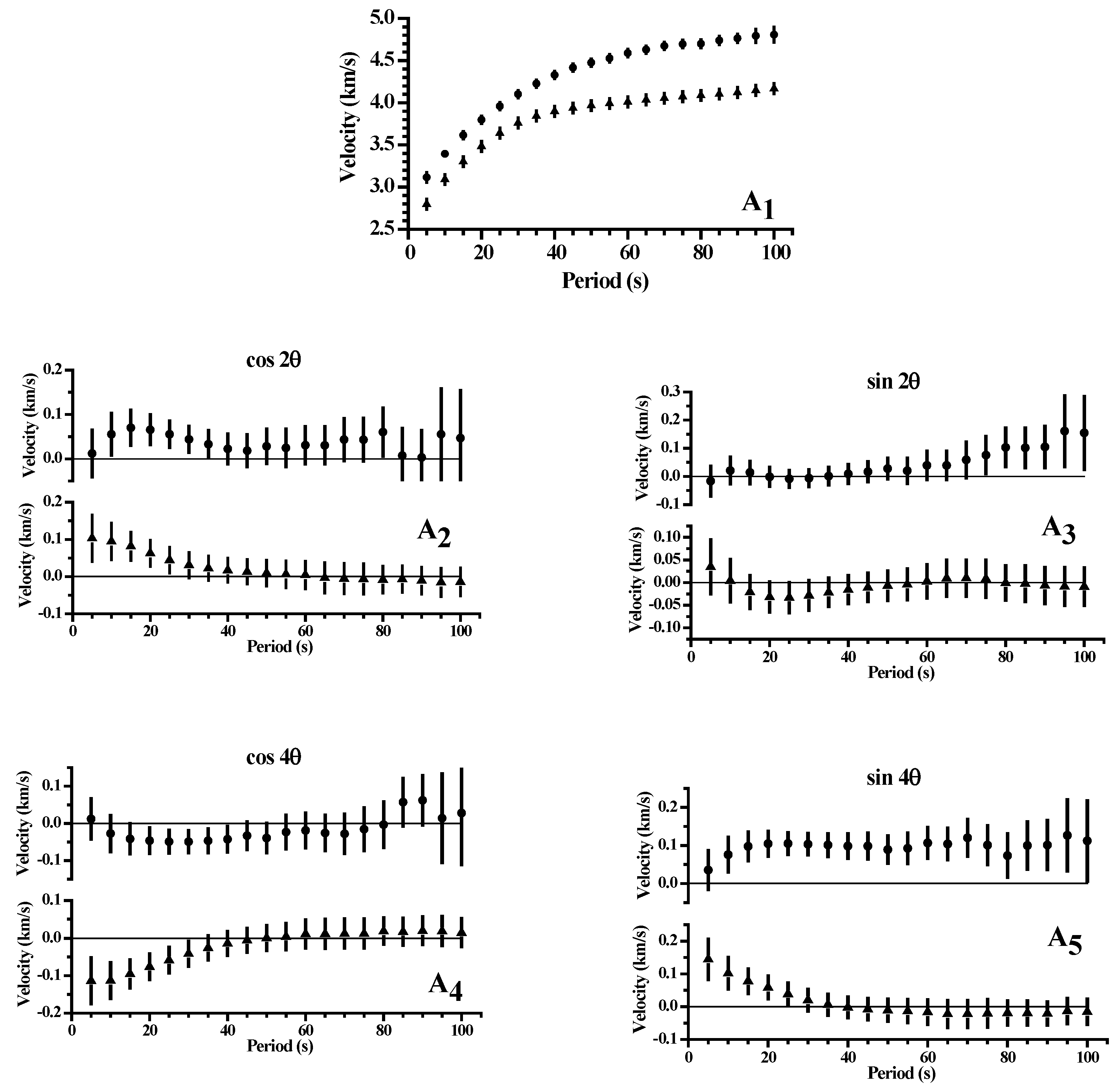
Figure 8.
(a) Error ε calculated by Formula (2), considering five (solid line) and three (dashed line) Ai coefficients in Formula (1). The red and magenta lines denote Love waves, and the blue and cyan lines denote Rayleigh waves. (b) Azimuthal variation in Love and Rayleigh phase velocities for the periods of 40 s. The solid lines show the phase velocity determined by Formula (1) with five (black line) and three (gray line) Ai coefficients. The small black circles denote Love waves and the small black triangles denote Rayleigh waves. The black vertical bars denote the standard deviation in phase velocity.

Figure 9.
(a) Schematic map of the study area [10]. The 1500 m isoline is plotted to show the elevated area resulting from the collision between the Arabian and Eurasian plates: the Turkish–Iranian continental plateau. OFZ: Oman folded zone, TZFZ—Taurus–Zagros folded zone. (b) Regions in which the seismic anisotropy will be determined (delimited by gray lines). The black circle denotes source zone (Supplement 3 and Figure 1a) and the black triangle denotes station (Supplement 2 and Figure 1a).

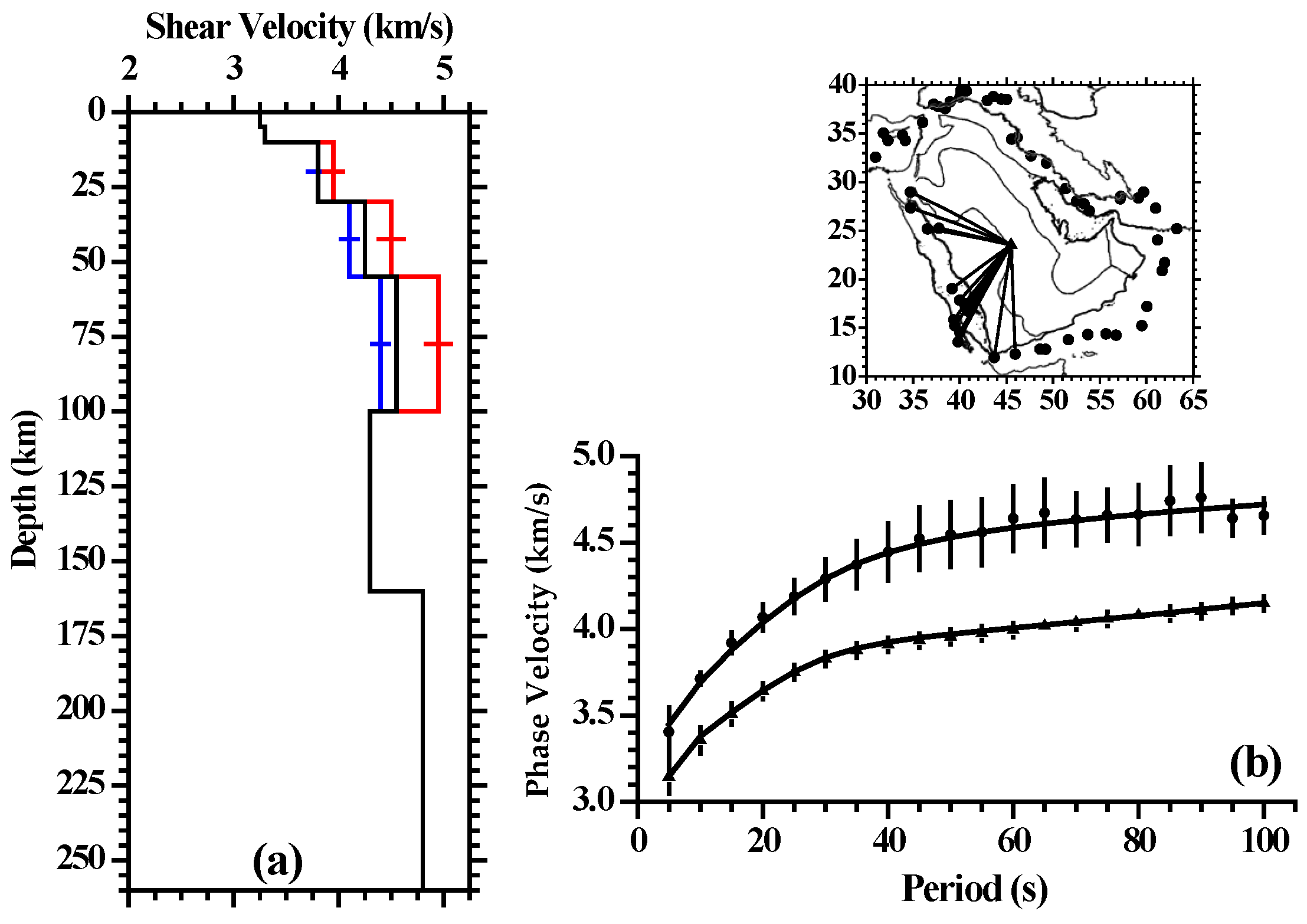
Figure 10.
Region 1: (a) The S-velocity distribution with depth of the initial model (Table 1) is plotted only from 0 to 260 km of depth. (b) The theoretical Love and Rayleigh phase velocities (continuous line), calculated from the initial model (Table 1), are compared with the Love (black circles) and Rayleigh (black triangles) phase velocities determined for this region. The vertical bars show the error in the phase velocities at each period (1-σ errors), for both Love and Rayleigh waves. (c) Resolving kernels calculated for the isotropic inversion of the Love and Rayleigh phase velocities. The reference depths are marked by vertical bars for the media depth of each layer considered.
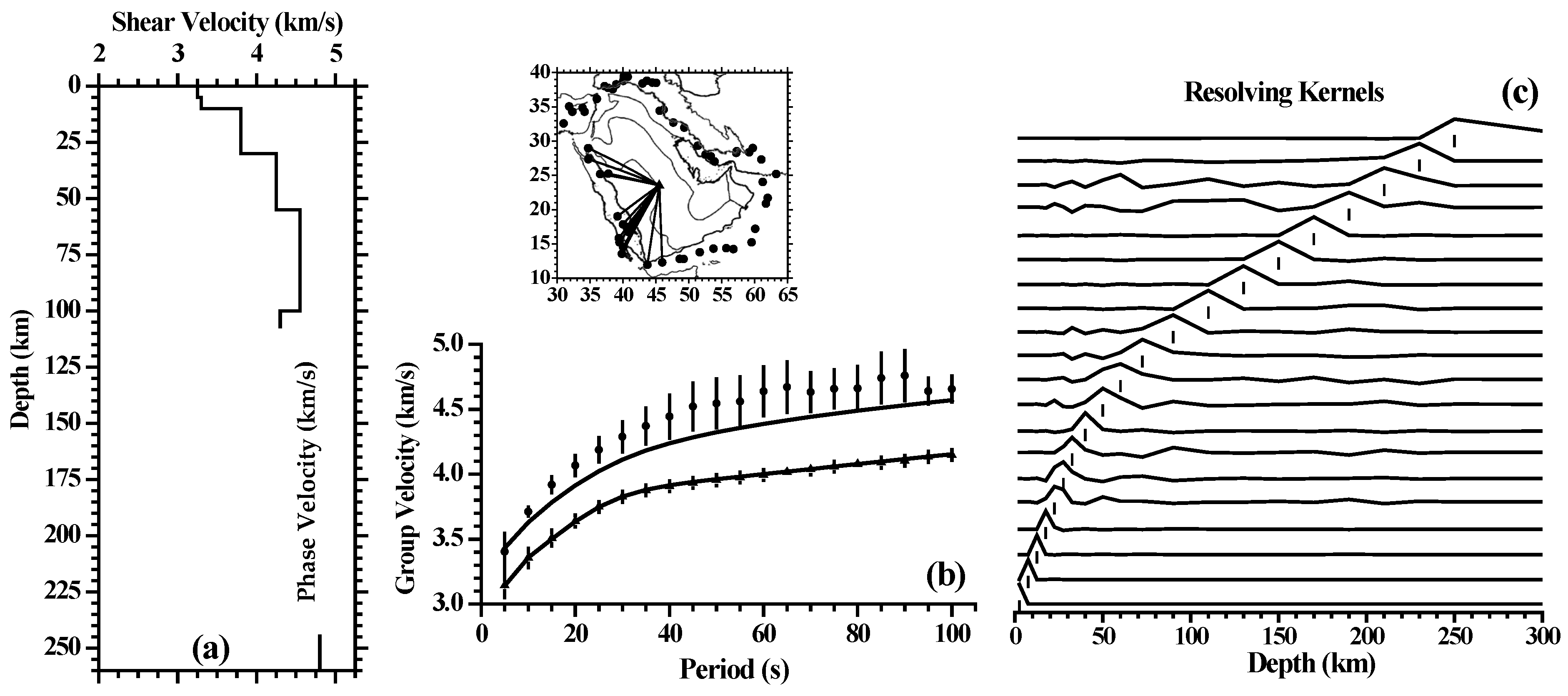
Figure 11.
Region 1: (a) The SV (blue line) and SH (red line) velocities, determined from anisotropic inversion, are compared with the isotropic S-velocity (black line, Table 1). (b) The theoretical Love and Rayleigh phase velocities (continuous line), calculated from the anisotropic model ((a), SV and SH velocities), are compared with the Love and Rayleigh phase velocities as in Figure 10. The vertical and horizontal bars have the same significance as Figure 10.

Table 1.
Region 1 (Figure 9b): Isotropic model considered as initial model (α: P-velocity, β: S-velocity and ρ: density) for the anisotropic inversion of the Love and Rayleigh phase velocities determined for this region.
Table 1.
Region 1 (Figure 9b): Isotropic model considered as initial model (α: P-velocity, β: S-velocity and ρ: density) for the anisotropic inversion of the Love and Rayleigh phase velocities determined for this region.
| Thickness (km) | α (km/s) | β (km/s) | ρ (g/cm3) |
|---|---|---|---|
| 5 | 5.63 | 3.25 | 2.30 |
| 5 | 5.72 | 3.30 | 2.77 |
| 20 | 6.58 | 3.80 | 2.85 |
| 25 | 7.36 | 4.25 | 3.20 |
| 45 | 7.88 | 4.55 | 3.35 |
| 60 | 7.45 | 4.30 | 3.40 |
| 100 | 8.31 | 4.80 | 3.53 |
| 140 | 8.31 | 4.80 | 3.60 |
| 100 | 9.41 | 5.09 | 3.64 |
| 100 | 9.72 | 5.26 | 3.84 |
| 40 | 9.97 | 5.26 | 4.08 |
| 30 | 10.54 | 5.70 | 4.16 |
| 130 | 10.68 | 5.85 | 4.22 |
| 200 | 11.10 | 6.26 | 4.43 |
| 200 | 11.48 | 6.44 | 4.61 |
| 200 | 11.78 | 6.54 | 4.74 |
| 200 | 12.06 | 6.64 | 4.83 |
| 12.32 | 6.75 | 4.92 |
Table 2.
Parameter ξ = (βH/βV)2 calculated for the regions shown in Figure 9b, from the SV (βV) and SH (βH) velocities shown in Figure 11a and Supplements F1a, F2a, F3a, F4a and F5a.
Table 2.
Parameter ξ = (βH/βV)2 calculated for the regions shown in Figure 9b, from the SV (βV) and SH (βH) velocities shown in Figure 11a and Supplements F1a, F2a, F3a, F4a and F5a.
| Depth (km) | Region 1 | Region 2 | Region 3 | Region 4 | Region 5 | Region 6 |
|---|---|---|---|---|---|---|
| 10–30 | 1.08 ± 0.08 | 1.05 ± 0.08 | 1.29 ± 0.10 | 1.25 ± 0.11 | 1.27 ± 0.10 | 1.05 ± 0.08 |
| 30–55 | 1.20 ± 0.10 | 1.02 ± 0.07 | 1.02 ± 0.07 | 1.00 ± 0.08 | 1.14 ± 0.07 | 1.05 ± 0.09 |
| 55–100 | 1.27 ± 0.10 | 1.14 ± 0.08 | 1.09 ± 0.07 | 1.09 ± 0.07 | 1.13 ± 0.07 | 1.00 ± 0.09 |
Disclaimer/Publisher’s Note: The statements, opinions and data contained in all publications are solely those of the individual author(s) and contributor(s) and not of MDPI and/or the editor(s). MDPI and/or the editor(s) disclaim responsibility for any injury to people or property resulting from any ideas, methods, instructions or products referred to in the content. |
© 2024 by the author. Licensee MDPI, Basel, Switzerland. This article is an open access article distributed under the terms and conditions of the Creative Commons Attribution (CC BY) license (https://creativecommons.org/licenses/by/4.0/).
Share and Cite
MDPI and ACS Style
Corchete, V. Azimuthal Variation in the Surface-Wave Velocity in the Arabian Plate. Appl. Sci. 2024, 14, 5142. https://doi.org/10.3390/app14125142
AMA Style
Corchete V. Azimuthal Variation in the Surface-Wave Velocity in the Arabian Plate. Applied Sciences. 2024; 14(12):5142. https://doi.org/10.3390/app14125142
Chicago/Turabian StyleCorchete, Víctor. 2024. "Azimuthal Variation in the Surface-Wave Velocity in the Arabian Plate" Applied Sciences 14, no. 12: 5142. https://doi.org/10.3390/app14125142
Note that from the first issue of 2016, this journal uses article numbers instead of page numbers. See further details here.