Abstract
To address the anti-swing issue of the payload in bridge cranes, Proportional–Integral–Derivative (PID) control is a commonly used method. However, parameter tuning of the PID controller relies on empirical knowledge and often leads to system overshoot. This paper proposes an Improved Sparrow Search Algorithm (ISSA) to optimize the gains of PID controllers, alleviating adverse effects on payload oscillation and trolley positioning during the operation of overhead cranes. First, tent map chaos mapping is introduced to initialize the sparrow population, enhancing the algorithm’s global search capability. Then, by integrating sine and cosine concepts along with nonlinear learning factors, the updating mechanism of discoverer positions is dynamically adjusted, expediting the solving process. Finally, the Lévy flight strategy is employed to update follower positions, thereby enhancing the algorithm’s local escape capability. Additionally, a fitness function containing overshoot penalties is proposed to address overshoot issues. Simulation results indicate that the overshoot rates of all algorithms remain less than 3%. Moreover, compared with the Sparrow Search Algorithm (SSA), Particle Swarm Optimization (PSO), Simulated Annealing (SA), and Whale optimization Algorithm (WOA), the optimized PID control system with the ISSA algorithm exhibits superior control performance and possesses certain robustness and adaptability.
1. Introduction
Bridge cranes play an indispensable role in modern factories as efficient handling equipment. Their flexibility, efficiency, and low impact on the floor and surrounding equipment make them essential handling tools in various types of factories. However, most industrial cranes still rely on manual operation, which often results in low efficiency and poor precision and can even cause the crane to swing due to the influence of the lifting mechanisms. This swinging can cause difficulties for operators in terms of system automation, thereby prolonging task completion times and reducing production efficiency. Therefore, anti-swing control of crane payloads and automatic trolley positioning technology have become key factors in improving the automation level of crane lifting operations.
In recent years, with the continuous improvement in industrial automation levels, the intelligent anti-swaying and positioning control of bridge crane systems has garnered significant attention and numerous control methods have been rapidly developed. These methods may differ in their basic objectives, but they can generally be categorized into two main types: closed-loop control [1,2,3] and open-loop control [4]. Open-loop control is relatively simple, as it only requires consideration of the input control signals without concerning the position of the crane trolley or the angle of the payload sway. Input shaping [5] is an open-loop technique used in real-time applications and has been widely applied in anti-swaying control for cranes. This technique achieves the reduction in system vibrations by convolving the command input signal with a series of pulses designed based on the system’s inherent frequency and damping ratio. Its fundamental principle lies in effectively suppressing vibrations that may occur within the crane system through meticulously designed pulse sequences, thereby enhancing system stability and control performance. The application of this method not only reduces vibration amplitudes but also improves the smoothness and precision of crane operation, thereby enhancing the efficiency and safety of the handling process. To address the impact of payload hoisting and the uncertainty of parameters, Cutforth and Pao [6] proposed an adaptive input shaping method based on flexible modal frequency variations. This method aims to cope with parameter uncertainties. Although input shaping techniques have achieved certain effectiveness in the anti-swaying control of cranes, their control targets are ideally determined using model parameters. Therefore, their performance may not be ideal when encountering external disturbances. Huang et al. [7,8] employed command smoothing techniques, coupled with dual pendulums and distributed mass payloads, to suppress oscillations in bridge cranes. Kim et al. [9] proposed an enhanced adaptive unscented Kalman filter. Simulations and practical experiments on a small-scale bridge crane system demonstrated that the proposed method is suitable for estimating payload swaying angles and friction forces.
Compared to open-loop control, closed-loop control allows for real-time and precise monitoring of both the payload swing angle and the position of the trolley during crane motion, enabling feedback control based on the acquired information. Therefore, in modern technological developments, the application of closed-loop control in crane sway suppression is becoming increasingly widespread. Yang and Xiong [10] employed the Linear Quadratic Regulator (LQR) method for the anti-sway control of overhead cranes. Adeli et al. [11] designed a parallel distributed fuzzy LQR controller combined with genetic algorithms for the anti-sway control of double-pendulum overhead cranes. Wang et al. [12] addressed the sway suppression and positioning issues of a double-pendulum bridge crane system by designing a novel time-varying sliding mode control (NTVSMC). This method effectively reduces the driving force of the trolley while ensuring rapid and accurate positioning, thereby suppressing the swinging of the payload sway angle. Guo et al. [13] devised a sliding mode control (SMC) method augmented with an extended state observer (ESO) for the positioning and two-stage swing suppression of a three-dimensional double-pendulum crane. Experimental findings demonstrate the method’s capability to achieve rapid and accurate positioning while effectively mitigating swing oscillations. Qiu et al. [14] proposed a disturbance observer for estimating external disturbances to address the adaptive fuzzy finite-time control problem based on disturbance observers for strict-feedback nonlinear systems. The effectiveness of this approach was verified through simulation studies on a single-link manipulator. Rubio et al. [15] proposed an observer-based differential evolutionary constraint control method for the safe reference tracking of robots. Qian et al. [16] proposed an enhanced anti-sway tracking control strategy based on adaptive neural networks for offshore crane systems, and the effectiveness of this method was validated through experiments. The PID control is a commonly used linear control technique in crane systems, where its three key parameters significantly influence the system’s stability and response characteristics. Therefore, selecting suitable parameters has become an important issue. In recent years, numerous scholars have devoted themselves to researching various intelligent optimization methods to achieve the optimization of PID parameters. Liu et al. [17] proposed a backpropagation neural network PID (BP-PID) control method for DC motor speed regulation. They compared its performance to the fuzzy PID (FPID) and traditional PID control methods, demonstrating its superiority. Xiao et al. [18] proposed a fuzzy PID control strategy optimized using the bee colony algorithm. The improved PID controller achieved excellent control precision in the torque control of magnetorheological (MR) clutches. Chen et al. [19] proposed a combined Cuckoo Search Optimization with an Improved Grey Wolf Optimization (CSO-IGWO) algorithm for tuning PID controller parameters. This algorithm utilizes the tent chaotic mapping method for population initialization and incorporates Lévy flight strategy to update position equations, enabling grey wolf individuals to make large jumps to expand the search space without easily becoming trapped in local optima. Fu et al. [20] combined the wandering lion optimization algorithm (LSO) with fuzzy PID control, introducing the LSO algorithm and incorporating a scattering operator, effectively enhancing its global search performance. This method reduces the probability of the algorithm becoming stuck in local optima and employs a nonlinear adaptive method to update inertia weights and learning coefficients. Rubio [21] proposed an improved bat control algorithm to enhance the trajectory tracking accuracy of robots. Experimental results indicate that the improved bat control algorithm achieved the best increase in trajectory tracking accuracy, and the proposed control method can be applied to other systems. Wang et al. [22] proposed an opposition-based learning jumping spider optimization algorithm to adjust the parameters of PID controllers, aiming to address the intelligent control problems related to the inlet flow rate, pressure, and temperature of heat exchangers in gas turbine cooling systems.
Since the sparrow search algorithm (SSA) proposal in 2020 [23], the SSA algorithm has been applied in many fields [24,25]. It mainly simulates the foraging behavior of sparrows to solve global optimization problems. Compared to other swarm intelligence optimization algorithms, the SSA algorithm has the characteristics of short learning time, high optimization accuracy, fast convergence speed, and good stability. However, in some cases, the SSA algorithm exhibits reduced search capability and decreased population diversity during the later stages of iteration, leading to drawbacks such as slow convergence speed, low solution accuracy, and susceptibility to local optima [26]. Therefore, improving the SSA algorithm has become a research hotspot. Qin et al. [27] combined the sparrow search algorithm with the traditional machine learning model Classification and Regression Trees (CART) to establish an SSA-CART optimization model for predicting pork prices. Jianhua and Zhiheng [28] proposed an optimization strategy that integrates the butterfly optimization algorithm (BOA). By improving the position updating strategy of the discoverers, the algorithm’s global exploration capability is enhanced. Xiong et al. [29] adopted an elite chaotic reverse learning strategy to generate the initial population and proposed an FOC-SSA algorithm. This algorithm improves the quality of initial individuals and population diversity to enhance the algorithm’s capability to escape local optima and convergence performance.
Based on the above research, it can be observed that with the continuous improvement in and application of metaheuristic algorithms, each algorithm has its unique advantages. Considering the novelty and limitations of the sparrow search algorithm (SSA), this study explored strategies suitable for addressing practical engineering problems and proposes a multi-strategy improved sparrow search algorithm (ISSA) combined with a PID controller to optimize controller gains. Firstly, by introducing tent chaotic mapping for initializing the sparrow population, the algorithm’s global search capability is enhanced while maintaining population diversity. Secondly, to tackle the slow convergence speed problem of the SSA algorithm when dealing with high-dimensional complex problems, the concepts of sine and cosine are combined, and a nonlinear learning factor is introduced to dynamically adjust the update mechanism of discoverer positions, thereby accelerating the solution process. Lastly, the Lévy flight strategy is employed to update follower positions, introducing perturbations and altering the current optimal solution, thereby enhancing the algorithm’s local escape capability. Additionally, addressing the common occurrence of overshoot in practical scenarios, a fitness function incorporating overshoot penalties is proposed to mitigate overshoot issues. This algorithm is then applied to optimize the PID controller parameters of a bridge crane. Through analysis of simulation results, the PID control system optimized by the ISSA algorithm demonstrates superior control performance compared to the SSA, PSO, SA, and WOA algorithms, while also exhibiting robustness and adaptability.
The content arrangement of this paper is as follows: Section 1 provides a general introduction. Section 2 elaborates on the theoretical model of the bridge crane, establishing its mathematical model using the Lagrangian equation. Section 3 innovatively introduces the SSA algorithm and its enhancements with multiple strategies. Section 4 describes how the ISSA algorithm is combined with PID controllers and applied to bridge crane control. Section 5 conducts simulations and analyses of the proposed method, examining the control effects of various algorithms on parameter variations and disturbances in bridge crane operations. Finally, conclusions are drawn in Section 6.
2. Mathematical Model of Bridge Crane
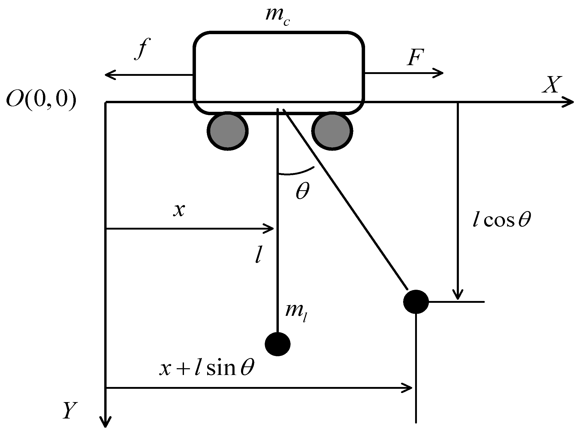
Many studies [30,31] have indicated that the coordinated motion of the trolley and crane can be decomposed and understood as independent two-dimensional motions. Focusing on the trolley’s motion allows the crane payload system to be simplified. As illustrated in Figure 1, the control system regulates the horizontal motion of the trolley on the bridge, thereby indirectly controlling the movement and sway of the payload by manipulating the trolley’s motion.

Figure 1.
Two-dimensional model of a bridge crane.
In practical operations, the crane is influenced by various factors, including the shape and mass of the payload, the length of the wire rope, external disturbances, and so on. This makes it a multivariable nonlinear system. Considering the complexity of mathematically modeling all these factors, in order to better establish motion models for studying sway suppression, it is necessary to simplify the system while ensuring that it conforms to engineering reality and sufficiently describes the system performance. By neglecting some relatively minor factors, the following assumptions are made about the system:
- Assumption 1: The motion of the trolley and the load is considered to be that of point masses.
- Assumption 2: During operation, the friction between the track and the wheels is proportional to the running speed. The effects of disturbances such as air resistance and wind force are neglected.
- Assumption 3: The driving force of the trolley is controllable, and the attenuation of transmission mechanisms such as motors is ignored.
The direction of the driving force acting on the trolley is defined as the positive horizontal direction (to the right) in the system, with the downward direction from the trolley’s center of mass designated as the positive vertical direction. The general form of the Lagrangian dynamics equations can be described as follows:
where is the Lagrangian operator, represents the kinetic energy, represents the potential energy, time is the independent variable, and the generalized coordinates (where = 1, 2, 3) are the dependent variables. Here, , , and , respectively, represent trolley position , payload swing angle , and length of the payload’s cable in Figure 1. represents the generalized external force acting on the generalized coordinate .
Using generalized coordinates to establish the differential equations for a system consisting of a three-degrees-of-freedom trolley and load, the mathematical model of the bridge crane hoisting system can be described as follows [32,33,34]:
where is the gravitational acceleration. Simplifying the system of Equations (1) and (2), we obtain the following:
Considering practical scenarios, bridge cranes often commence lifting operations only after the load has been raised to a predetermined height, and lowering of the load occurs once both the trolley and the load have reached their designated positions. Thus, the deformation of the wire rope can be disregarded, denoted as . Furthermore, to ensure safety, the sway angle is typically kept minimal, especially near the stable point, where it approximates , as derived from Equation (3):
Taking the Laplace transform of both sides of Equation (4), we obtain the following:
Simplifying Equation (5), the transfer functions for the position of the trolley and the swing angle of the load can be obtained.
where denotes the transfer function for the trolley position, where the input is the trolley driving force, and the output is the trolley position. Meanwhile, represents the transfer function for the load swing angle, where the input is the trolley driving force, and the output is the payload swing angle.
3. Multi-Strategy Improved Sparrow Search Algorithm
3.1. Traditional Sparrow Search Algorithm
The sparrow population is primarily composed of discoverers and followers. Discoverers assist the sparrow population in locating food and guiding them to food sources, while followers accompany the discoverers to obtain food. Additionally, a portion of individuals in the sparrow population are randomly selected as sentries. Sentries emit warnings upon detecting danger, prompting the entire sparrow flock to flee to safety. The sparrow aggregation matrix is as follows:
where represents the quantity of sparrows in the population, represents the dimension of the variable, . The fitness function is used to evaluate the performance or adaptability of each sparrow individual and is a critical component of optimization algorithms. The fitness function of the sparrow population is represented by Equation (8):
Each in denotes the adaptability of an individual. Sparrows with superior adaptability are given precedence in obtaining food and function as foragers, guiding the entire population towards the food source. The updating mechanism for the discoverers’ positions is outlined as follows:
where represents the position of the sparrow in the dimension. denotes the number of iterations of the population. stands for the maximum iteration times of the population. represents a random number within the range . represents a random number following a normal distribution within the range . represents a matrix of size , where each element in the matrix has a value of 1. and , respectively, represent the warning value and the safe value. When , it indicates that the sparrows have not detected any predators during the foraging process and can continue to expand the search for prey over a large area; otherwise, it indicates that predators of the sparrow population have started to appear, and the entire sparrow population needs to fly quickly to other areas.
Apart from discoverers, most sparrows are followers, which obtain food by following the discoverers. The update rule for the follower’s position is given by Equation (10):
In the equation, represents the global best position, represents the global worst position, is a matrix, and . When , it indicates that the ith follower has a higher fitness value and can obtain sufficient food; otherwise, it means that its fitness value is lower and it needs to go elsewhere to replenish food.
In order to ensure the safety of the population, a small portion of individuals in the sparrow population are selected as sentries. The position updating method for sentries is given by Equation (11):
where is a randomly generated number with a controllable step size following a normal distribution within the range . represents the sparrow’s movement direction, which is a uniformly distributed random number within the range . , and represent the fitness values of individual sparrows, the global optimal fitness value, and the global worst fitness value, respectively. is a small constant to avoid division by zero. indicates that the sparrow is at the edge of the population, making it vulnerable to predator attacks.
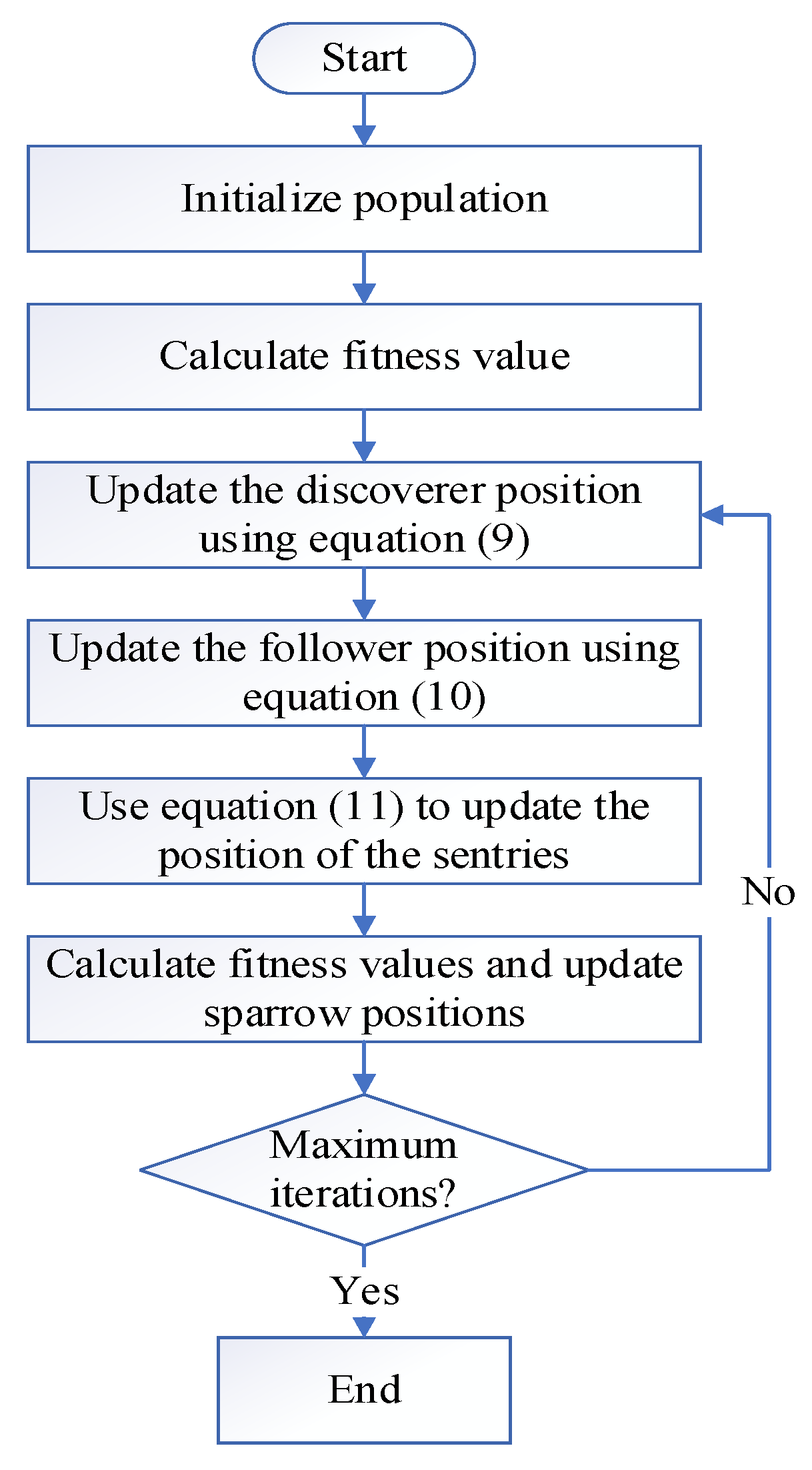
The flowchart of the traditional SSA is illustrated in the Figure 2.
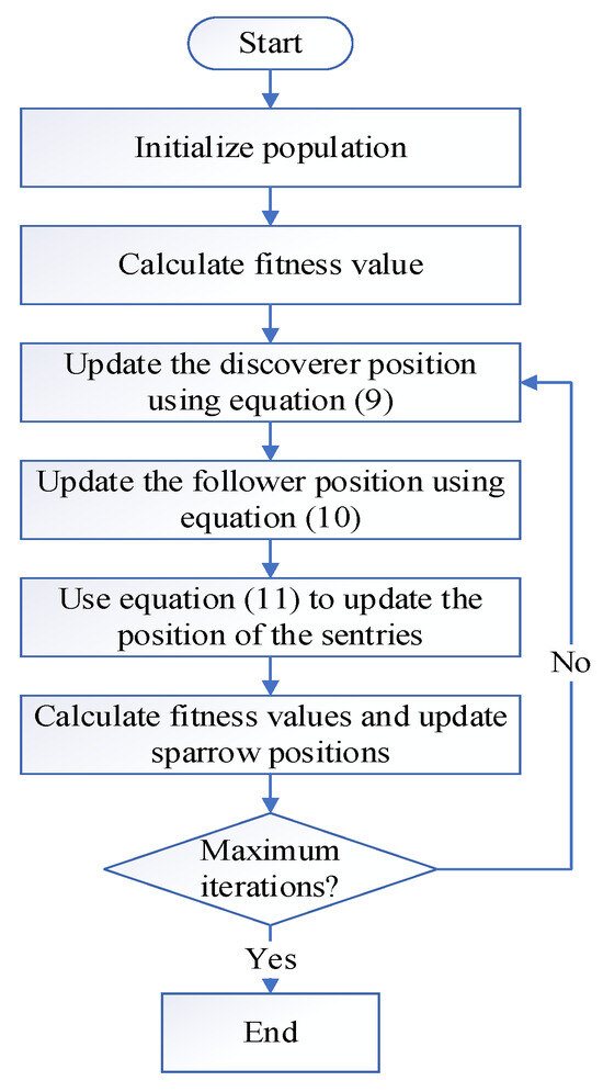
Figure 2.
Sparrow search algorithm flowchart.
3.2. Proposed ISSA Algorithm
3.2.1. Tent Chaotic Map Strategy
The tent chaotic map strategy [35] is an initialization method used in optimization algorithms. This strategy leverages the characteristic that the traversal of the tent chaotic map is uniform and random. This makes it easier for the algorithm to escape local optima and enhances its global search capability. Therefore, introducing the tent chaotic map strategy helps maintain population diversity and improves the convergence speed and optimization accuracy of the algorithm. The equation is as follows:
where is a random point between 0 and 1, and represents the current iteration number. Mapping the variable values generated by the tent chaotic map to the sparrow individuals yields the initialization of the overall tent chaotic population.
In the equation, represents the mapped individual; and denote the upper and lower bounds for each individual and each dimension, respectively. is the tent chaotic sequence generated according to Equation (12).
3.2.2. Incorporating the Ideas of the Sine–Cosine Algorithm
In the basic SSA algorithm, when the fitness of sparrow individuals falls below the threshold , the positions of discoverers gradually shrink with the increase in iterations, leading to the convergence of the search space and increasing the risk of falling into local optimal solutions. To address this issue, we incorporate the idea of the sine–cosine algorithm (SCA) [36,37] into the updating process of the discoverers’ positions and we introduce a nonlinear sine learning factor. In the early stages of the search, the learning factor has a relatively large value, facilitating global exploration. Conversely, in the later stages of the search, the learning factor has a smaller value, aiding in enhancing local exploration capability and optimization accuracy.
The nonlinear sine learning factor as in Equation (14) is as follows:
The equation for the updated positions of discoverers after improvement are shown below:
In Equation (15), is a random number in the range , and is another random number in the range .
3.2.3. Lévy Flight Strategy
The Lévy flight strategy is a random search algorithm that follows the Lévy distribution, achieving a balance between short-distance exploration and occasional long-distance movements. In the traditional SSA optimization process, when the discoverers iterate a certain number of times without a change in fitness value, followers will take over as new discoverers. This transition may lead to issues such as compromised global search capability, limited local development, and susceptibility to local optima. To mitigate the risk of falling into local optima, we introduce the Lévy flight strategy into the follower update equation. This strategy enhances the flexibility of individual position changes, expands the search space, and helps prevent the algorithm from becoming stuck, thus maintaining the discoverers’ effective global search capability.
The updated equation for the follower’s position is as follows:
where represents the current best position occupied by the discoverer. The mechanism of Lévy flight is as follows:
where and are random numbers within a range , and the value of can be taken as 1.5. The calculation method for is as follows:
where .
3.2.4. General Framework of ISSA
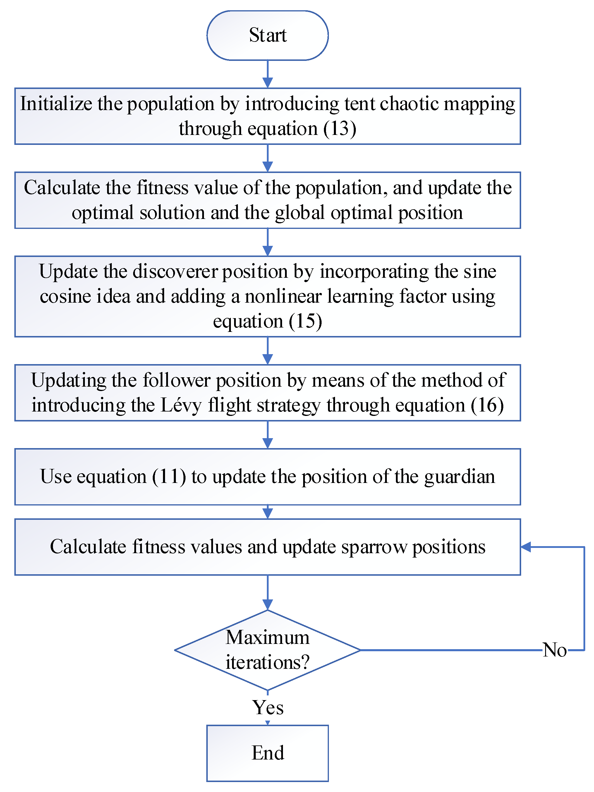
The ISSA algorithm first initializes the population using tent chaotic mapping to enhance population diversity. Next, it integrates the sine–cosine concept and introduces a nonlinear learning factor to dynamically adjust the update mechanism of the discoverer’s position, thereby accelerating the solution rate. Finally, the ISSA algorithm introduces the Lévy flight strategy into the follower’s position updating method to perturb and mutate the current optimal solution, enhancing local escape capabilities.
Step 1: Initialize algorithm parameters, including population size , dimension , discoverers , sentinels , warning value , upper bound , lower bound , and maximum iteration number .
Step 2: Initialize the entire population using the tent chaotic sequence from Equation (12), generating -dimensional vectors , then map them to the variable range of the original problem space using Equation (13).
Step 3: Compute the fitness of each sparrow, then select the current optimal fitness value and its corresponding position .
Step 4: Select the top sparrows with strong adaptability as discoverers, and the rest as followers. After incorporating the sine–cosine algorithm (SCA) idea and introducing a dynamic learning factor, update the discoverer’s position according to Equation (15).
Step 5: The remaining sparrows act as followers, introducing the Lévy flight strategy and updating the follower’s position based on Equation (16).
Step 6: Randomly select sparrows from the sparrow population as sentries and update their positions according to Equation (11).
Step 7: After one iteration, recalculate the fitness value of each sparrow and the average fitness value of the entire sparrow population.
Step 8: Based on the current status of the sparrow population, update the optimal position and its fitness value experienced by the entire population.
Step 9: Check if the algorithm meets the termination conditions. If yes, end the algorithm and output the results; otherwise, return to Step 4.
The flowchart of the ISSA is illustrated in the Figure 3.
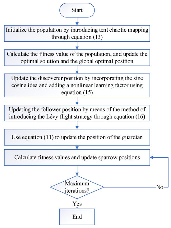
Figure 3.
Improved sparrow search algorithm flowchart.
3.3. Performance of ISSA
To validate the improved performance and effectiveness of the ISSA, we employed the CEC-2005 test suite for evaluation. The CEC-2005 suite comprises a set of challenging benchmark functions characterized by intricate local optima, effectively simulating the complexity of real search spaces. Testing on these benchmark functions allows for a comprehensive assessment of algorithmic performance and robustness. Some of the benchmark functions are listed in Table 1.

Table 1.
Benchmark test functions.
F1–F7 represent multi-dimensional unimodal functions, which are typically difficult to solve and are suitable for evaluating the solving and optimization capabilities of algorithms. Meanwhile, F8–F13 represent multi-dimensional multimodal functions, characterized by multiple local optimal points and barriers, and are suitable for evaluating the ability of algorithms to escape local optimal values.
The experiments were conducted on an Intel(R) Core(TM) i5-12600KF processor running at 3.70 GHz, with 32.00 GB of RAM, using the Windows 10 operating system and MATLAB R2022b. During the evaluation of the ISSA algorithm, it was compared against SSA and three other widely respected metaheuristic algorithms (SA, WOA, and PSO). By statistically analyzing the results from 30 independent runs, we could gain a more accurate understanding of the ISSA’s performance relative to other algorithms. Through the repeated debugging and operation of all algorithms, the parameter values are as shown in Table 2.
Table 2.
Parameter values of five algorithms.
The experimental results are based on datasets obtained from 30 independent runs for each benchmark test function. We utilize the average value and standard deviation for the 13 test functions as the final performance evaluation metrics. These metrics are presented in Table 3.
Table 3.
ISSA and optimization results of other algorithms (SSA, PSO, SA, WOA) in test functions.
Table 3 presents the mean and standard deviation of results obtained from 30 independent runs of five algorithms on benchmark test functions under 30-dimensional conditions. A smaller mean indicates the better optimization performance of the algorithm, while the standard deviation reflects the system’s stability. As shown in Table 3, ISSA generally outperforms the other four algorithms in terms of search accuracy and optimization stability for both unimodal and multimodal benchmark test functions. Compared to classical optimization algorithms and their improved versions, ISSA exhibits significant advantages in solution accuracy and robustness. This indicates that the proposed ISSA effectively improves upon SSA. Therefore, the proposed ISSA algorithm demonstrates robustness and reliable performance in solving complex optimization problems.
4. Design of Adaptive PID Controller Based on ISSA
4.1. Traditional PID Controller
In the field of control systems, the PID (Proportional–Integral–Derivative) control algorithm, as a classic feedback control method, is widely employed to regulate the dynamic performance of systems. The PID controller adjusts the control output based on the current error (difference between setpoint and actual value) and the rate of change of the error , aiming to achieve stability, rapid response, and precise tracking of targets.
The PID controller consists of proportional, integral, and derivative terms, corresponding to the current error, accumulated past errors, and the rate of change of the error, respectively. The proportional term generates the control output by adjusting the error magnitude, the integral term eliminates steady-state errors by accumulating the error over time, and the derivative term predicts the future trend based on the rate of change of the error, thereby suppressing oscillations and enhancing system stability. The PID controller is represented by Equation (19).
In the Equation (19), represents the proportional coefficient, denotes the integral time constant, and stands for the derivative time constant. The schematic diagram of the PID control system is depicted in Figure 4.
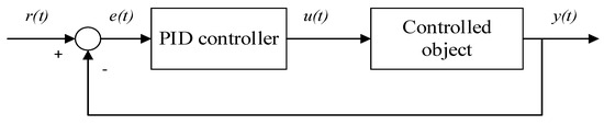
Figure 4.
Schematic diagram of the PID control system.
In Figure 4, represents the desired output, denotes the controller output, and stands for the actual output.
4.2. Improved Adaptive PID Controller
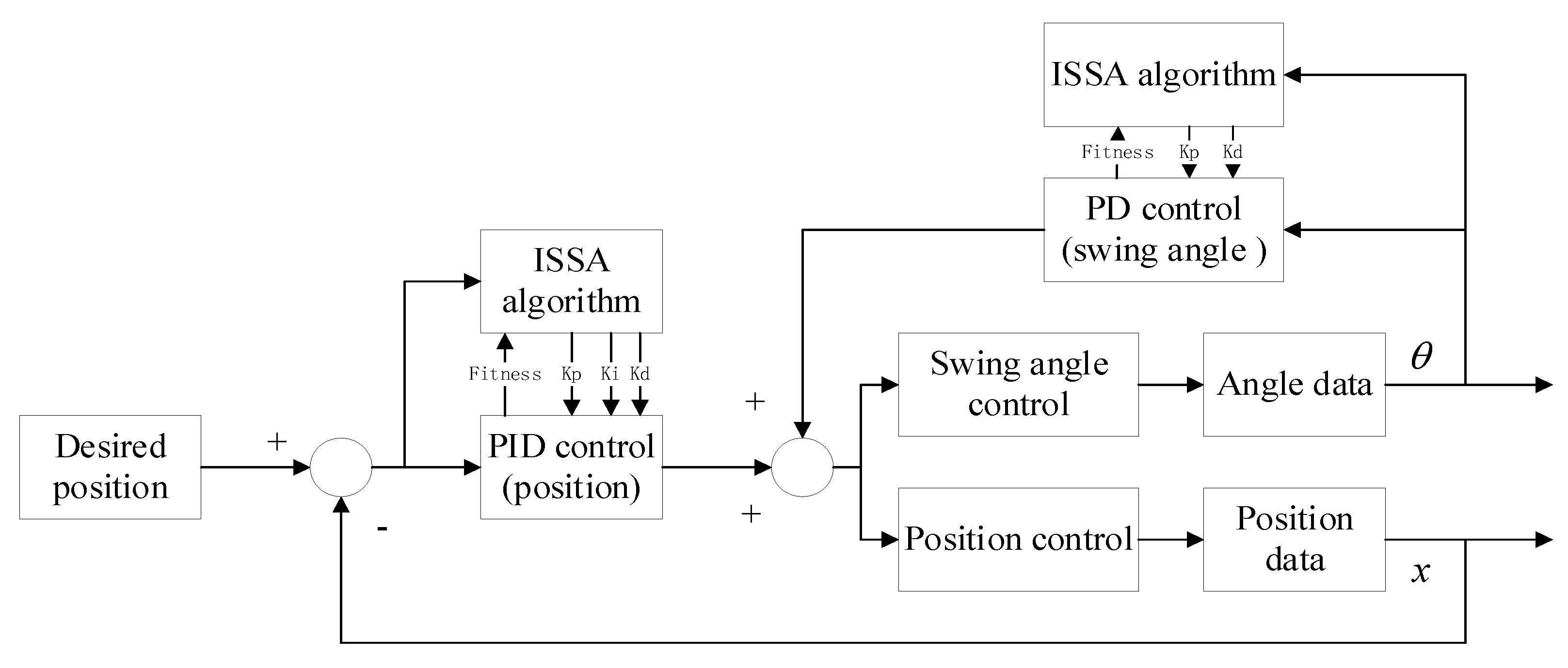
The performance of a PID controller is highly dependent on its three parameters. Determining these parameters typically involves adjustment based on empirical knowledge or experimentation, a method that often consumes significant time and effort and may result in unstable performance or suboptimal control effects. In the anti-swing control system of a bridge crane, which represents a single-input multiple-output system, the outputs include the position of the trolley and the swinging angle of the lifting load. Consequently, the system designed in this study adopts a dual-loop feedback control model. Within this model, the optimization objective is to find a set of PID values that minimize the error by optimizing the three parameters. PID control is chosen for trolley position control due to its requirement for high precision and elimination of steady-state errors, while PD control is selected for payload swing angle control because it necessitates quick response and oscillation suppression. The schematic diagram of the PID control system based on the ISSA algorithm is depicted in Figure 5.
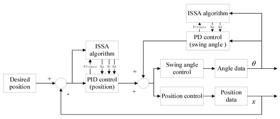
Figure 5.
Improved bridge crane PID control system with ISSA algorithm.
5. Simulation Experiments
5.1. Overshoot Optimization Methods
Each initial particle generated by the intelligent algorithm contains a total of five parameters: , , and in the PID controller, as well as and in the PD controller. The intelligent algorithm is integrated with the simulation model of the bridge crane PID control system, enabling simulation analysis of the PID controller model to derive the dynamic performance indicators of the system. Throughout the iteration process, the dynamic performance indicators of the system serve as adaptive fitness values transmitted to the intelligent algorithm program. The adaptive fitness value determines whether the termination condition of the algorithm is met. If the termination condition is satisfied, the iteration concludes, and the optimal solution is returned. Otherwise, the iteration computation continues, repeating the preceding parameter-setting steps until the optimal PID controller parameters are determined.
The optimal PID gains are determined by minimizing the objective function. There are typically four performance indices used to evaluate system performance [38]: (1) Integral of Squared Error ; (2) Integral of Absolute Error ; (3) Integral of Time multiplied by Squared Error ; (4) Integral of Time multiplied by Absolute Error . Generally, each system aims to reduce error, minimize overshoot, and enhance response speed. In this study, the is employed as the performance evaluation criterion, as it enables the system to exhibit rapid response characteristics. The expression for the fitness function is as follows:
where represents the difference between the output and input of the control system, while denotes the simulation time. Additionally, considering the necessity of limiting overshoot in crane position, a penalty term is introduced when the overshoot of the crane position controller exceeds 0. Assuming the system comprises two outputs and two controllers, the expression for fitness is as follows:
where and represent the errors of the crane position controller and the swing angle suppression controller, respectively. denotes the fitness function for all algorithms in the experiment. is a control value employed to prevent excessive control margins. and are weighting factors for adjusting the effect of different errors on the fitness function, typically ranging from 0 to 1. In this study, and are set to 0.95. is another weighting factor, also typically ranging from 0 to 1. In this study, is set to 0.05. represents the overshoot penalty coefficient. When the error in the trolley position is greater than 0, a larger will have a greater effect on the fitness value, and a calibrated value with a larger overshoot will result in a worse fitness value. In this study, is set to 100.
5.2. Simulation and Analysis
In this section, the parameters of two PID controllers were set using methods such as ISSA, SSA, PSO, SA, and WOA to validate the optimization effectiveness of the proposed algorithms. A simulation control system for each optimization method was established using the SIMULINK module in MATLAB, and the control performance obtained from each parameter-setting method was compared and analyzed under common conditions. By iteratively manually adjusting the parameters of the PID controller beforehand, the range of variation for each parameter could be approximately determined, thereby significantly reducing the scope of PID parameter optimization. The parameter ranges of the PID controller obtained through repeated testing and operation are shown in Table 4.
Table 4.
Parameter ranges for PID and PD controllers.
To evaluate the control performance of the designed bridge crane PID control system, the expected position signal of the crane trolley is set to a step signal of 5 m, and the initial swing angle of the crane payload is set to 0°. The simulation time is set to 30 s, and the solver is chosen to be variable step size. The parameter values of the crane are shown in Table 5.
Table 5.
Parameters of the bridge crane system.
The improved PID controllers generated by five intelligent algorithms were connected to the bridge crane control system, and the iteration curves are illustrated in Figure 6. The performance index functions of the ISSA, SSA, PSO, SA, and WOA algorithms were recorded as 17.03, 18.64, 37.15, 24.05, and 22.11, respectively. The performance index function value achieved by the ISSA algorithm was the smallest among all algorithms, exhibiting an improvement of 8.64% in search accuracy compared to the SSA algorithm. The iteration count was reduced by 10.77% to 58 iterations. Compared to the PSO, SA, and WOA algorithms, the performance index function values decreased by 20.02, 7.02, and 5.08, respectively, for the ISSA algorithm. These results suggest that the proposed ISSA algorithm holds a certain advantage over other algorithms in terms of iteration count and precision. The values of the PID parameters calculated by the five algorithms are shown in Table 6.
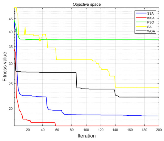
Figure 6.
Iterative curves of ISAA, SSA, PSO, SA, and WOA algorithms.
Table 6.
Parameters of bridge crane PID controllers obtained by ISSA, SSA, PSO, SA, and WOA algorithms.
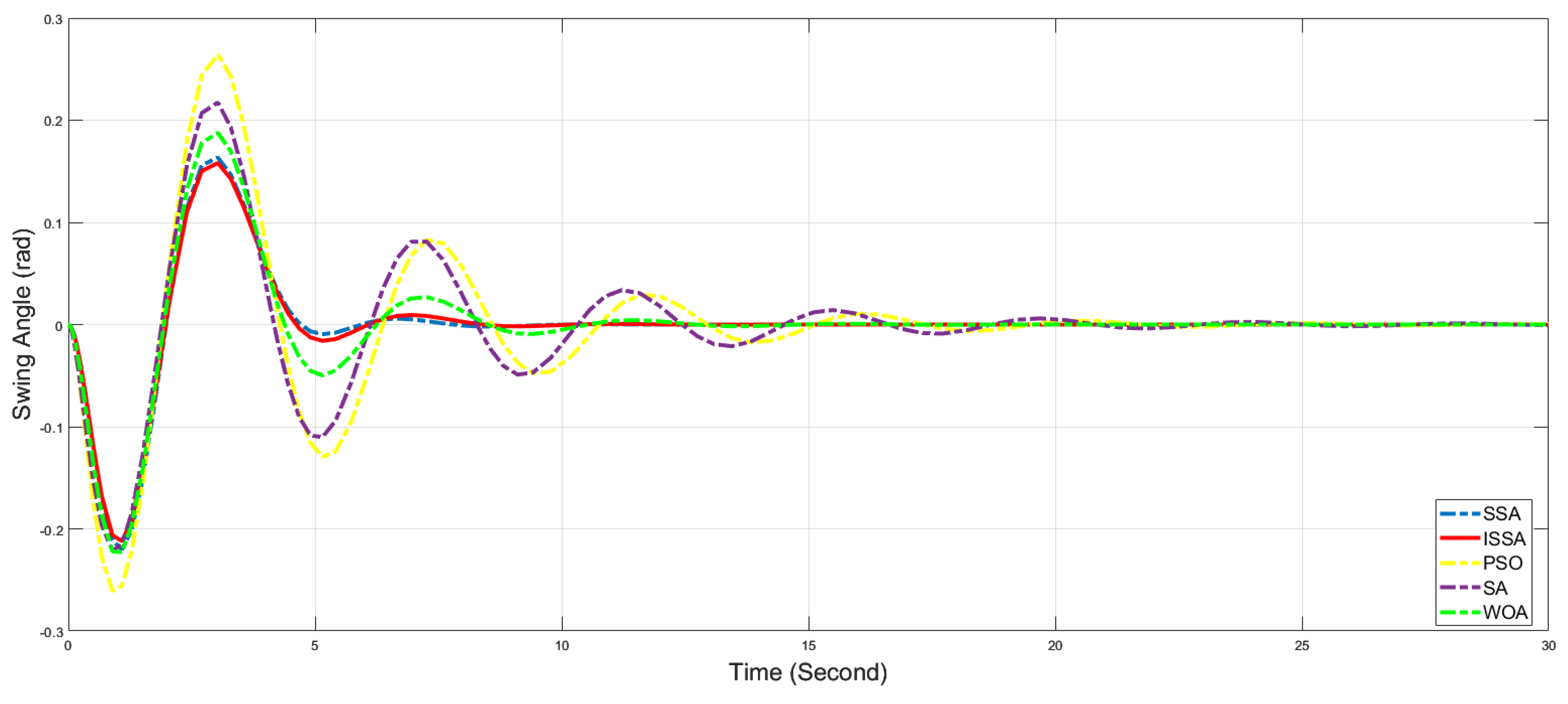
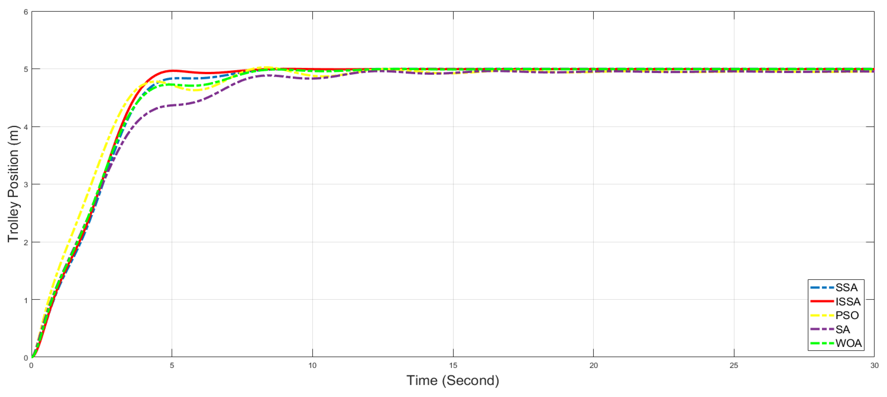
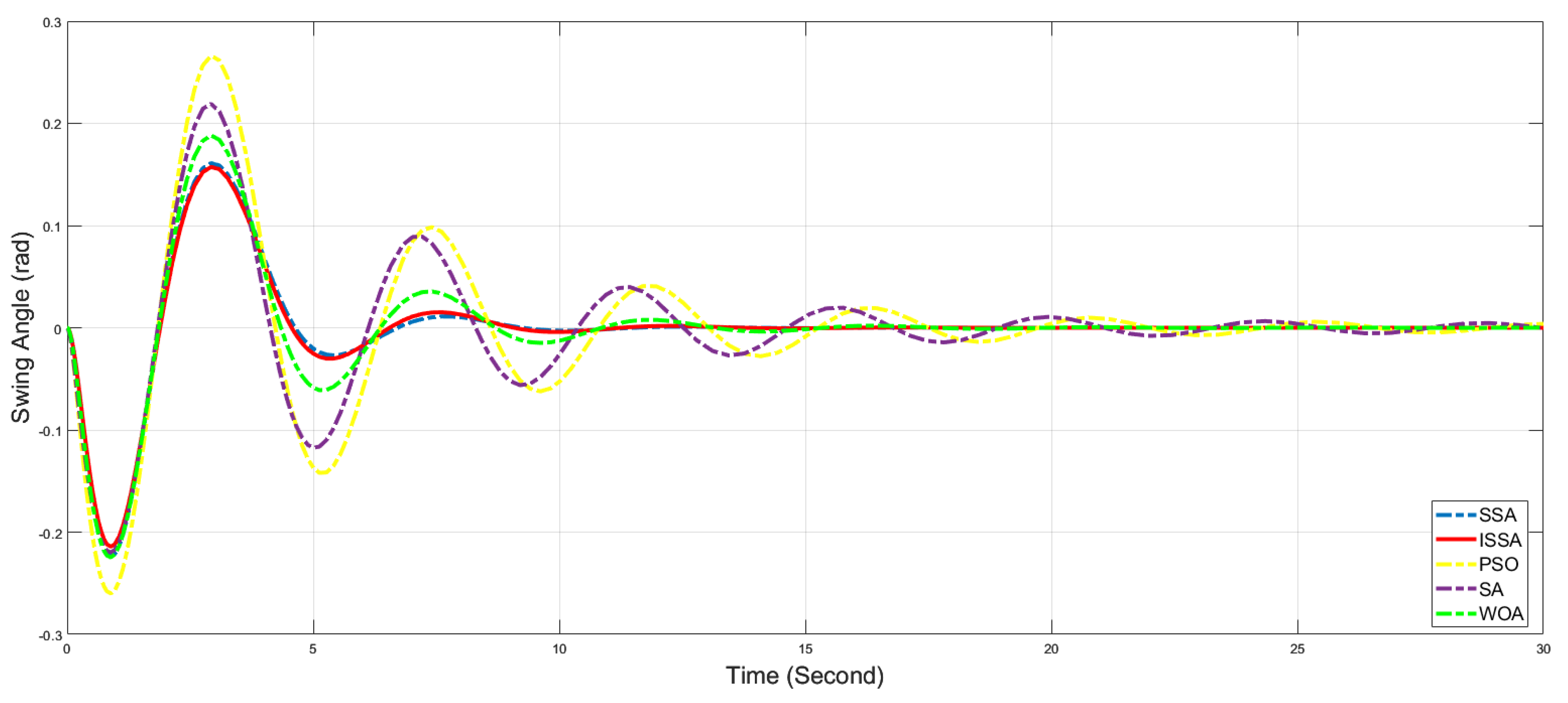
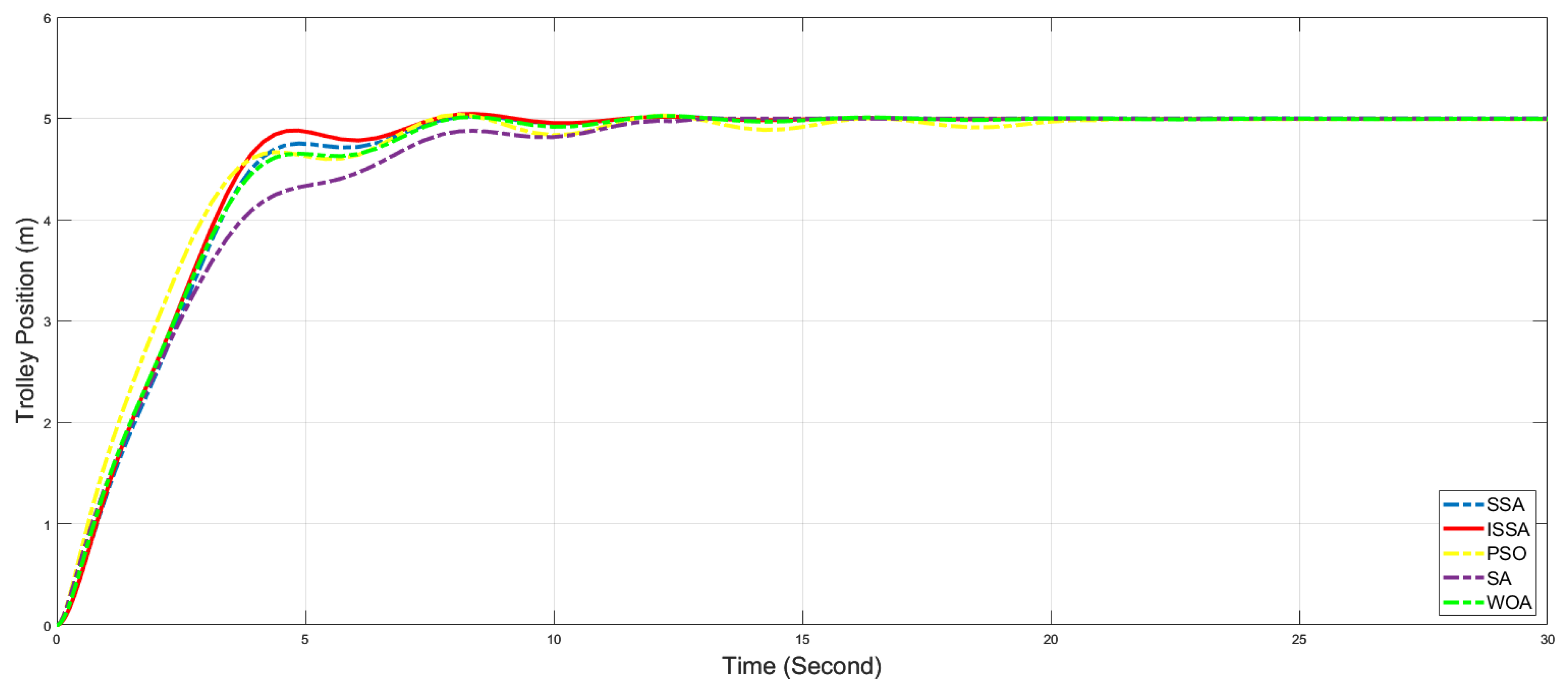
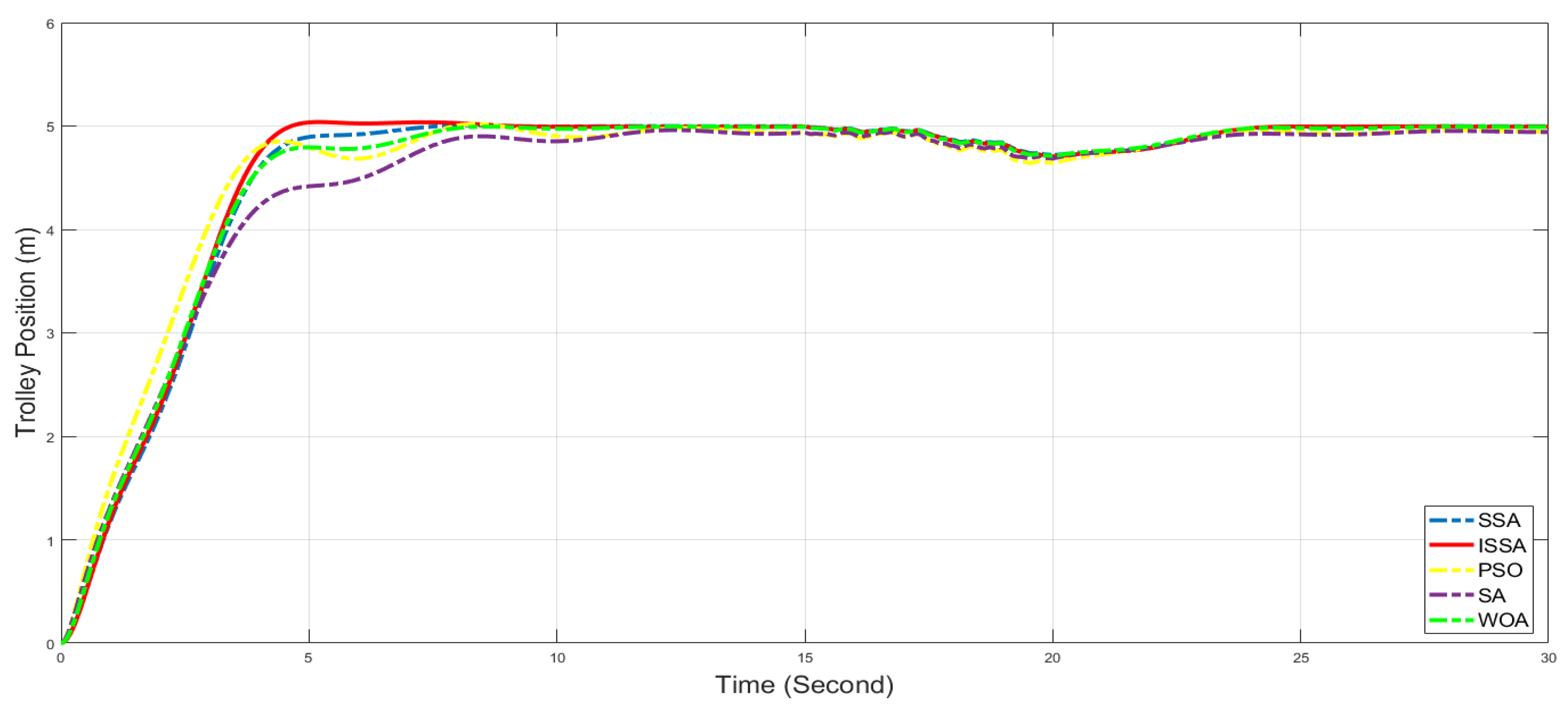
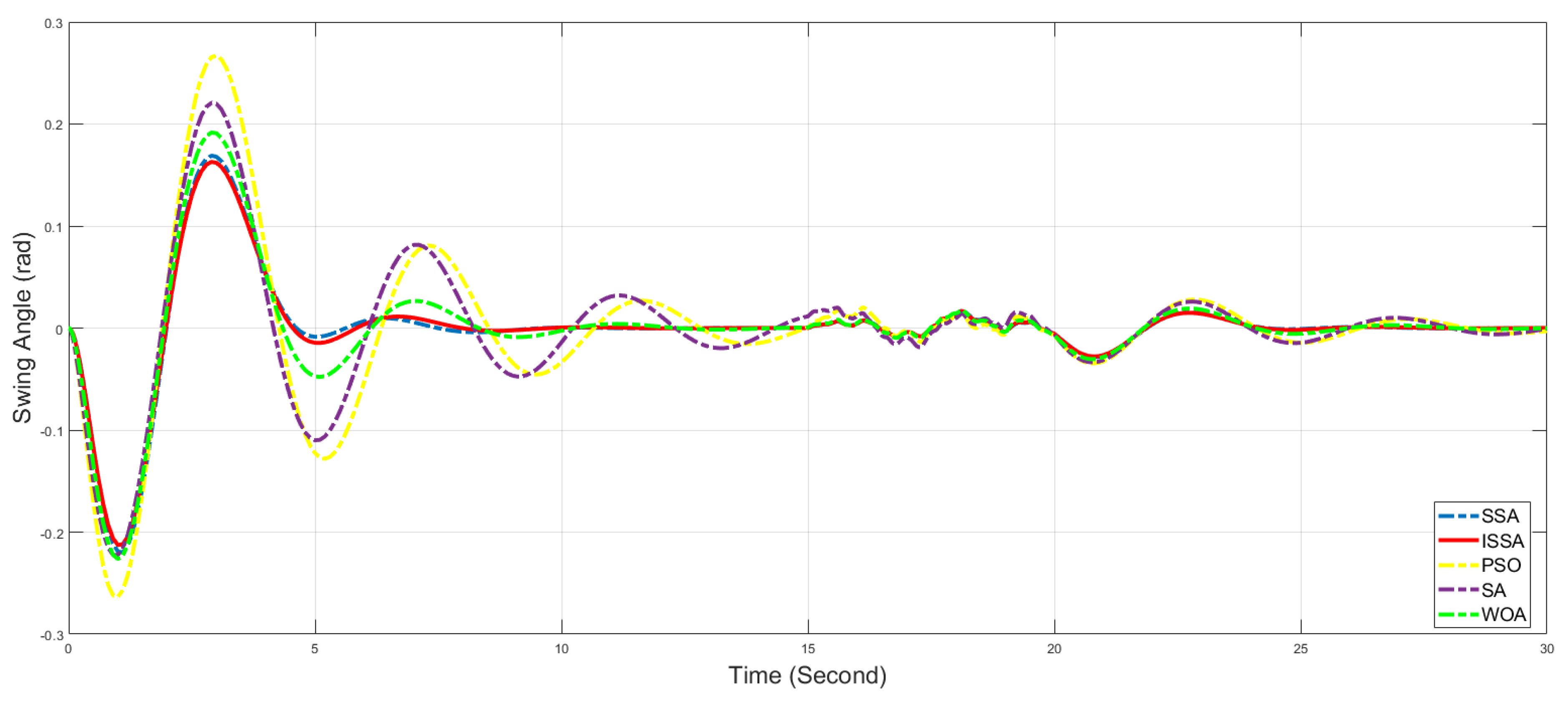
The outputs of trolley position and payload swing angle obtained by the ISSA, SSA, PSO, SA, and WOA algorithms are shown in Figure 7 and Figure 8, respectively. The performance metrics of the five algorithms are shown in Table 7.
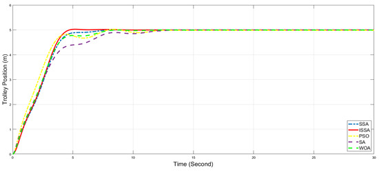
Figure 7.
Trolley position control effects for five algorithms.

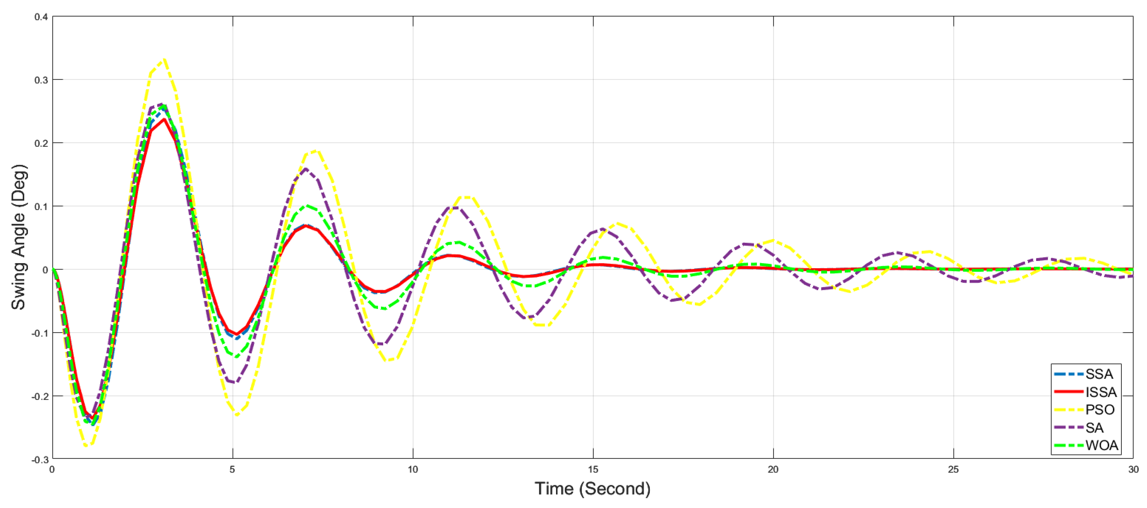
Figure 8.
Payload swing angle suppression effects of five algorithms.
Table 7.
Performance index of PID control systems improved by five algorithms.
In the position curves of the trolley, the peak times for the ISSA, SSA, PSO, SA, and WOA algorithms are 5.074 s, 7.904 s, 8.268 s, 12.392 s, and 8.673 s, respectively, while the steady-state times are 4.791 s, 7.379 s, 15.586 s, 12.837 s, and 8.632 s, respectively. Among these algorithms, the ISSA algorithm exhibits the smallest peak time and steady-state times, followed by the SSA and WOA algorithms. Conversely, the PSO algorithm requires the longest time to stabilize after reaching the peak, needing 7.378 s. Furthermore, the ISSA algorithm demonstrates the smallest steady-state error of 0.002, followed by the SSA, WOA, SA, and PSO algorithms, with errors of 0.006, 0.006, 0.048, and 0.050, respectively. These results indicate that the ISSA algorithm performs well in controlling the trolley position, meeting the positional control requirements of the bridge crane system effectively. In the payload swing angle curves, the maximum swing angles for the SSA, PSO, SA, and WOA algorithms are 0.163, 0.264, 0.217, and 0.188, respectively, while for the ISSA algorithm, it is 0.158, which is lower than that of the other four algorithms. Additionally, the ISSA algorithm exhibits a steady-state time for the payload swing angle of 9.382, which is smaller compared to 0.011 s, 12.142 s, 13.384 s, and 4.893 s for the other four algorithms, respectively. Both the maximum swing angle and steady-state time of the ISSA algorithm are the smallest, indicating its effectiveness in suppressing the payload swing angle in bridge crane applications.
Experimental data show that after incorporating overshoot penalty terms into the fitness function, none of the control curves for the crane’s trolley position exhibit overshoot for any of the five algorithms. Furthermore, the PID controller optimized by the ISSA algorithm demonstrates excellent control performance in the bridge crane control system, indicating its superior suitability for both trolley positioning control and payload swing angle suppression compared to the other four algorithms.
5.3. Robustness Simulation Experiments
In practical operating scenarios, certain parameters of a bridge crane may incur errors due to measurement methods and environmental variations. Therefore, to evaluate the adaptability and stability of the PID gains obtained by each optimization technique, simulations of the crane control systems using the five algorithms were conducted under different operating conditions. The parameters corresponding to each of the five scenarios are listed in Table 8.
Table 8.
Parameters of bridge crane control systems under five other working conditions.
Figure 9, Figure 10, Figure 11, Figure 12, Figure 13, Figure 14, Figure 15, Figure 16, Figure 17 and Figure 18 illustrate the trolley position and payload swing obtained by the five algorithms under five different working conditions. The values of the performance index of the five algorithms under these conditions are presented in Table 9. In the position curves under conditions 1 to 5, the ISSA algorithm exhibits the smallest peak time among the four algorithms, with values of 5.014, 9.147, 8.247, 6.070, and 8.147, respectively. Under conditions 2 and 4, all five algorithms demonstrate no overshoot. However, in conditions 1 and 5, the PSO algorithm experiences overshoot, measuring 0.46% and 0.72%, respectively. In condition 3, four algorithms exhibit overshoot, with PSO having the highest value of 0.7%. Across all five scenarios, ISSA showcases shorter settling times and lower steady-state errors compared to the other four algorithms, with values of 7.101 and 0.002, 7.715 and 0.002, 7.469 and 0.005, and 7.136 and 0.002, respectively. In the payload swing angle curves for the five scenarios, ISSA consistently demonstrates the shortest settling time for the maximum swing angle compared to the other four algorithms, with values of 0.156 and 10.836, 0.157 and 11.030, 0.236 and 16.194, and 0.189 and 11.687, respectively.
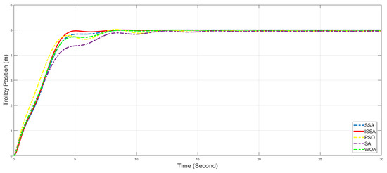
Figure 9.
Trolley position control effects for five algorithms under working condition 1.
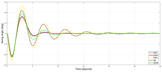
Figure 10.
Payload swing angle suppression effects for five algorithms under working condition 1.
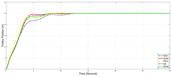
Figure 11.
Trolley position control effects for five algorithms under working condition 2.
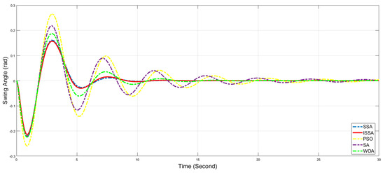
Figure 12.
Payload swing angle suppression effects for five algorithms under working condition 2.
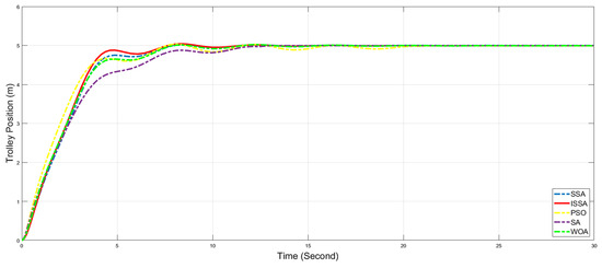
Figure 13.
Trolley position control effects for five algorithms under working condition 3.
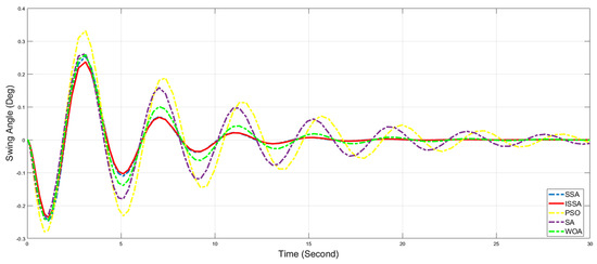
Figure 14.
Payload swing angle suppression effects for five algorithms under working condition 3.
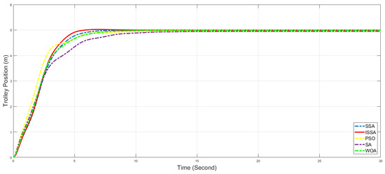
Figure 15.
Trolley position control effects for five algorithms under working condition 4.
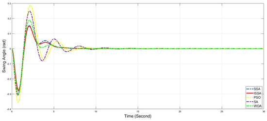
Figure 16.
Payload swing angle suppression effects for five algorithms under working condition 4.
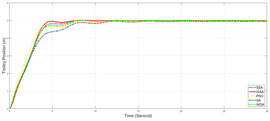
Figure 17.
Trolley position control effects for five algorithms under working condition 5.
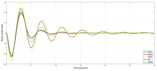
Figure 18.
Payload swing angle suppression effects for five algorithms under working condition 5.
Table 9.
Performance index of five algorithms under five working conditions.
These findings suggest that, following the integration of overshoot penalty terms into the fitness function, the occurrence of overshoot in the position curves across the five scenarios is notably reduced for all five algorithms, with overshoot values consistently below 1%. This indicates that the devised fitness function effectively suppresses overshoot. Furthermore, in comparison to the SSA, PSO, SA, and WOA algorithms, the PID control optimized by the ISSA algorithm demonstrates enhanced adaptability and stability, enabling effective control performance in bridge crane control systems across diverse operational scenarios.
5.4. Anti-Disturbance Simulation Experiments
Additionally, during practical operations, bridge cranes often encounter various sources of disturbances. These disturbances may stem from operator commands or external environmental uncertainties such as wind forces, fluctuations in payloads, and environmental noise, among others. These disturbances can potentially affect the crane’s performance and lead to deterioration or failure of the control system. To validate the robustness of the algorithm, disturbance tests were conducted on the system to simulate its responses under different disturbances and influences. The algorithm’s resistance to disturbances was evaluated accordingly.
To simulate the effects of wind forces and environmental noise on bridge cranes operating outdoors, white noise was added to the feedback signal during the simulation period of 15–20 s. Figure 19, Figure 20, Figure 21 and Figure 22 illustrate the trolley position and effective payload swing angle curves of the bridge crane under two types of white noise disturbances. Table 10 presents the performance indicators of the system after being subjected to disturbances. In Figure 19 and Figure 21, the ISSA algorithm demonstrates the minimum peak time and steady-state time, measuring 15.825 and 24.058, and 24.248 and 23.016, respectively. In Figure 20 and Figure 22, the maximum swing angle achieved by the ISSA algorithm is 0.052 and 0.014, respectively, both lower than the corresponding values for the other four algorithms. The steady-state times are 24.403 and 25.299, respectively, both lower than the PSO algorithm’s 10.149 and 9.104. It can be observed that under external disturbances, the ISSA algorithm exhibits the optimal response and recovery speeds among the five algorithms, demonstrating the favorable stability of the bridge crane system controlled by the ISSA algorithm-optimized PID controller in the presence of disturbances.

Figure 19.
Trolley position control effects for five algorithms under white noise 1.
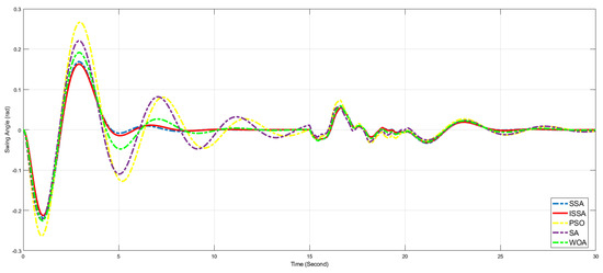
Figure 20.
Payload swing angle suppression effects for five algorithms under white noise 1.
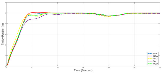
Figure 21.
Trolley position control effects for five algorithms under white noise 2.
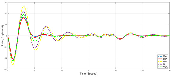
Figure 22.
Payload swing angle suppression effects for five algorithms under white noise 2.
Table 10.
Performance index of five algorithms under two types of noise.
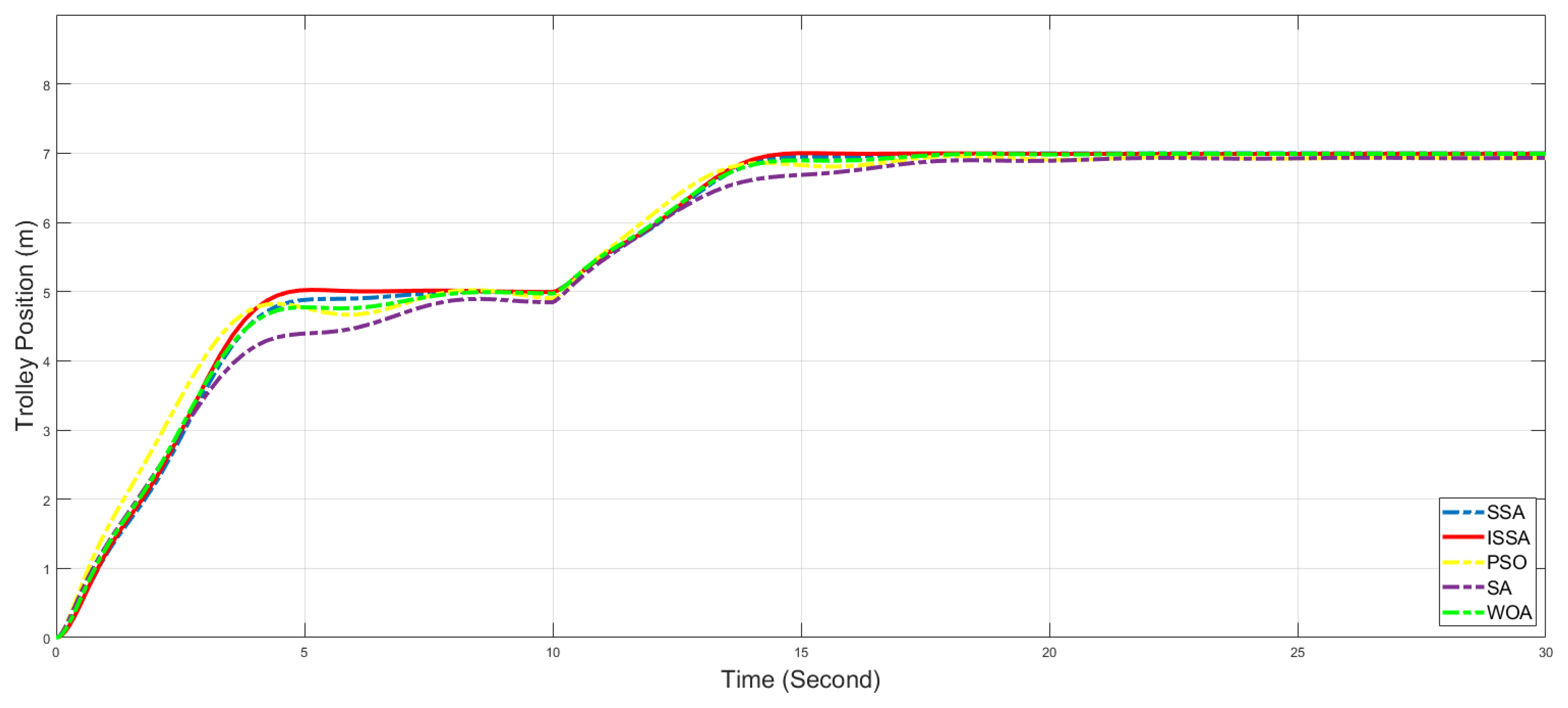
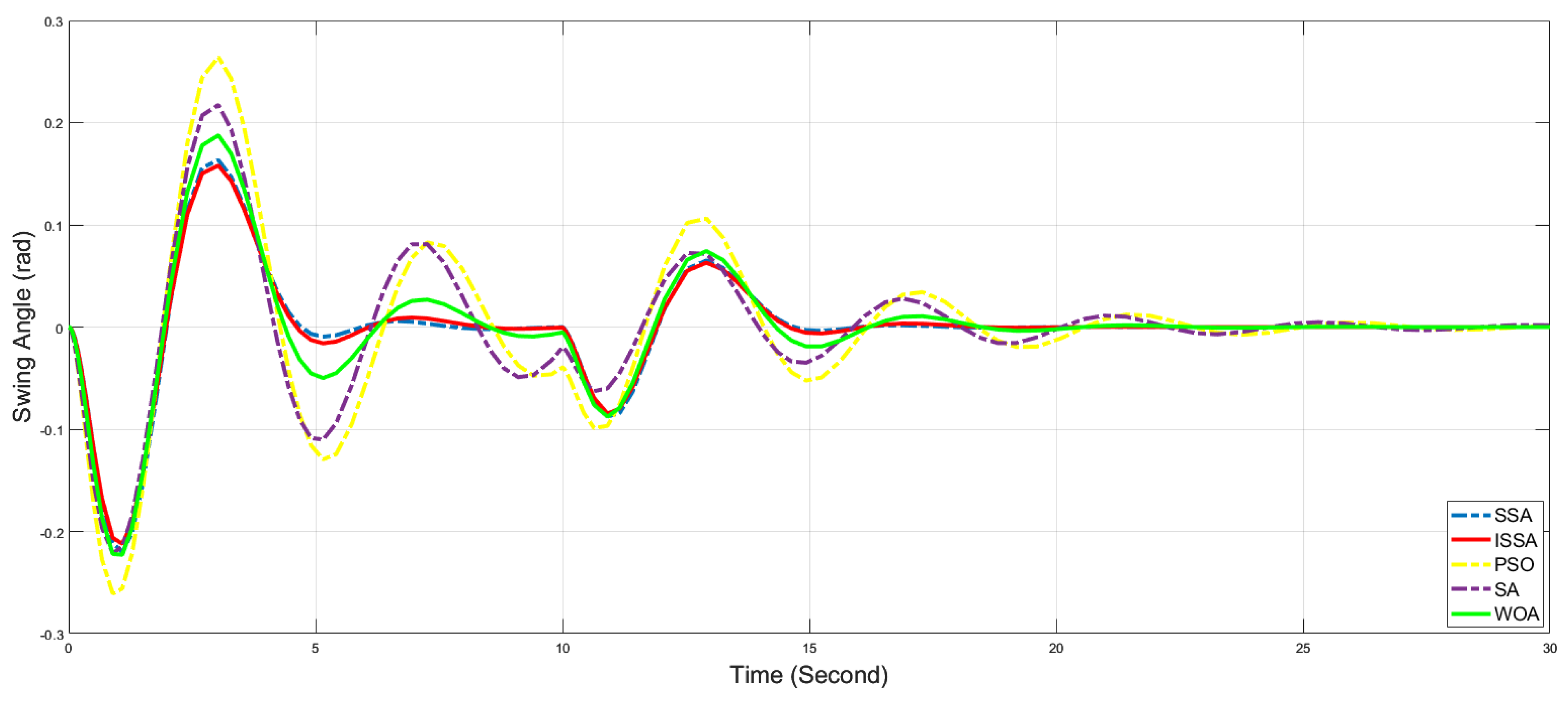
At = 10 s during simulation, a step signal with a magnitude of 2 is introduced into the expected position signal of the trolley to simulate the requirement of operator command change. Figure 23 and Figure 24 depict the trolley position curve and payload swing angle curve, respectively, after the input command change. The parameters of the bridge crane system are provided in Table 11. Following the change in the expected position of the trolley, the ISSA algorithm exhibits the smallest peak time and the shortest steady-state time among the five algorithms, with values of 14.905 s and 14.495 s, respectively. The maximum swing angle of the payload is 0.063, with a steady state time of 18.471 s, both of which are smaller than the corresponding values for the other four algorithms. It is evident that the ISSA algorithm demonstrates faster response and recovery speeds than the other four algorithms following the receipt of operator command change, indicating the better stability of the bridge crane control system when using the ISSA algorithm in the event of input signal variations.
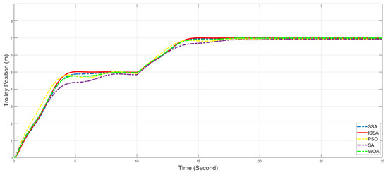
Figure 23.
Trolley position control effects of the five algorithms after input command variations.
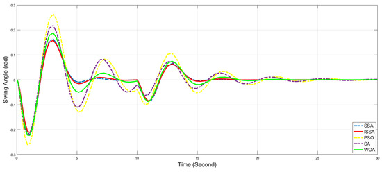
Figure 24.
Payload swing angle suppression effects of the five algorithms after input command variations.
Table 11.
Performance index of the five algorithms after input command variations.
6. Conclusions
This paper proposes an improved Sparrow Search Algorithm (ISSA) for optimizing the PID parameters of a bridge crane control system. Firstly, the traditional Sparrow Search Algorithm is enhanced by introducing Tent Map Chaos during the initialization phase of the algorithm iteration to enhance the quality of initial solutions. Additionally, the algorithm integrates the concepts of the sine–cosine algorithm and introduces a nonlinear learning factor to adjust the position updating mechanism of discoverers, thereby enhancing both local exploitation and global exploration capabilities. The Lévy flight strategy is introduced to improve the follower’s position updating method, enhancing its ability to escape local optima. Finally, to address overshoot in the trolley position of the crane, an overshoot penalty term is introduced into the fitness function. Comparative analysis with existing PSO, SA, WOA, and SSA algorithms demonstrates that the ISSA algorithm exhibits more precise search capability while meeting the convergence requirements.
The application of the proposed algorithm to the control system revealed experimental results indicating that the overshoot of all five algorithms was less than 5%, underscoring the effectiveness of the improved fitness function. Furthermore, in comparison with other algorithms, the ISSA algorithm demonstrated superior performance in both trolley position control and effective suppression of payload swing angle. When subjected to varying working conditions and external disturbances, the ISSA algorithm exhibited the fastest response time and shortest steady-state time. These findings validate the robustness and high performance of the ISSA algorithm. Consequently, the PID controller optimized using the ISSA algorithm can be effectively employed for trolley position control and payload swing angle suppression in bridge crane systems, thereby satisfying the control requirements of such systems.
Subsequent research will combine other control methods of the proposed ISSA, such as fuzzy control and neural networks, and apply them to more complex systems, such as crane double-pendulum systems, power generation, and so on.
Author Contributions
Conceptualization, Y.Z. and L.L.; methodology, Y.Z. and L.L.; software, Y.Z., L.L. and J.L.; validation, Y.Z., L.L., J.L., J.C., C.K. and D.H.; formal analysis, Y.Z. and L.L.; investigation, Y.Z. and L.L.; resources, Y.Z. and L.L.; data curation, Y.Z., L.L., J.L., J.C., C.K. and D.H.; writing—original draft, Y.Z. and L.L.; writing—review and editing, Y.Z., L.L., J.L. and C.K.; visualization, Y.Z. and L.L.; supervision, Y.Z. and L.L.; project administration, Y.Z. and L.L. All authors have read and agreed to the published version of the manuscript.
Funding
This research was funded by the University-Industry Cooperation Project “Research and Application of Intelligent Traveling Technology for Steel Logistics Based on Industrial Internet”, grant number 2022H6005; Natural Science Foundation of Fujian Provincial Science and Technology Department, grant number 2022J01952; Research Start-up Projects, grant number GY-Z12079; Fujian University Industry-University Cooperation Science and Technology Programme, grant number 2022N5020.
Institutional Review Board Statement
Not applicable.
Informed Consent Statement
Not applicable.
Data Availability Statement
The data presented in this study are available on request from the corresponding author. The data are not publicly available due to privacy.
Conflicts of Interest
The authors declare no conflicts of interest.
References
- Rubio, J.D.J.; Hernandez, M.A.; Rosas, F.J.; Orozco, E.; Balcazar, R.; Pacheco, J. Genetic high-gain controller to improve the position perturbation attenuation and compact high-gain controller to improve the velocity perturbation attenuation in inverted pendulums. Neural Netw. 2024, 170, 32–45. [Google Scholar] [CrossRef] [PubMed]
- Xie, X.; Wei, C.; Gu, Z.; Shi, K. Relaxed Resilient Fuzzy Stabilization of Discrete-Time Takagi–Sugeno Systems via a Higher Order Time-Variant Balanced Matrix Method. IEEE Trans. Fuzzy Syst. 2022, 30, 5044–5050. [Google Scholar] [CrossRef]
- García-Chávez, R.E.; Silva-Ortigoza, R.; Hernández-Guzmán, V.M.; Marciano-Melchor, M.; Orta-Quintana, Á.A.; García-Sánchez, J.R.; Taud, H. A Robust Sliding Mode and PI-Based Tracking Control for the MIMO “DC/DC Buck Converter–Inverter–DC Motor” System. IEEE Access 2023, 11, 119396–119408. [Google Scholar] [CrossRef]
- Al-Fadhli, A.; Khorshid, E. A smooth optimized input shaping method for two-dimensional crane systems using Bezier curves. Trans. Inst. Meas. Control. 2021, 43, 2512–2524. [Google Scholar] [CrossRef]
- Fujioka, D.; Shah, M.; Singhose, W. Robustness analysis of input-shaped model reference control on a double-pendulum crane. In Proceedings of the American Control Conference, Chicago, IL, USA, 1–3 July 2015; pp. 2561–2566. [Google Scholar]
- Cutforth, C.F.; Pao, L.Y. Adaptive input shaping for maneuvering flexible structures. Automatica 2004, 40, 685–693. [Google Scholar] [CrossRef]
- Huang, J.; Liang, Z.; Zang, Q. Dynamics and swing control of double-pendulum bridge cranes with distributed-mass beams. Mech. Syst. Signal Process. 2015, 54–55, 357–366. [Google Scholar] [CrossRef]
- Huang, J.; Xie, X.; Liang, Z. Control of Bridge Cranes with Distributed-Mass Payload Dynamics. IEEE/ASME Trans. Mechatron. 2015, 20, 481–486. [Google Scholar] [CrossRef]
- Kim, J.; Lee, D.; Kiss, B.; Kim, D. An Adaptive Unscented Kalman Filter with Selective Scaling (AUKF-SS) for Overhead Cranes. IEEE Trans. Ind. Electron. 2020, 68, 6131–6140. [Google Scholar] [CrossRef]
- Yang, B.; Xiong, B. Application of LQR Techniques to the Anti-Sway Controller of Overhead Crane. Adv. Mater. Res. 2010, 139–141, 1933–1936. [Google Scholar] [CrossRef]
- Adeli, M.; Zarabadipour, H.; Zarabadi, S.H.; Shoorehdeli, M.A. Anti-swing control for a double-pendulum-type overhead crane via parallel distributed fuzzy LQR controller combined with genetic fuzzy rule set selection. In Proceedings of the 2011 IEEE International Conference on Control System, Computing and Engineering, Penang, Malaysia, 25–27 November 2011. [Google Scholar]
- Wang, T.; Tan, N.; Zhou, J.; Zhang, X.; Zhang, J. A Novel Sliding Mode Control Method for Double Pendulum Crane. In Proceedings of the 3rd International Conference on Information Technologies and Electrical Engineering 2020, Changde, China, 3–5 December 2020. [Google Scholar]
- Guo, Q.; Chai, L.; Liu, H. Anti-swing sliding mode control of three-dimensional double pendulum overhead cranes based on extended state observer. Nonlinear Dyn. 2023, 111, 391–410. [Google Scholar] [CrossRef]
- Qiu, J.; Wang, T.; Sun, K.; Rudas, I.J.; Gao, H. Disturbance Observer-Based Adaptive Fuzzy Control for Strict-Feedback Nonlinear Systems with Finite-Time Prescribed Performance. IEEE Trans. Fuzzy Syst. 2022, 30, 1175–1184. [Google Scholar] [CrossRef]
- de Jesús Rubio, J.; Orozco, E.; Cordova, D.A.; Hernandez, M.A.; Rosas, F.J.; Pacheco, J. Observer-based differential evolution constrained control for safe reference tracking in robots. Neural Netw. 2024, 175, 106273. [Google Scholar] [CrossRef] [PubMed]
- Qian, Y.; Hu, D.; Chen, Y.; Fang, Y.; Hu, Y. Adaptive Neural Network-Based Tracking Control of Underactuated Offshore Ship-to-Ship Crane Systems Subject to Unknown Wave Motions Disturbances. IEEE Trans. Syst. Man Cybern. Syst. 2021, 52, 3626–3637. [Google Scholar] [CrossRef]
- Liu, L.; Zhang, Y.; Chen, J.; Chen, J. Research and Application of Control Algorithm Based on Intelligent Traveling Crane. In Proceedings of the 2023 IEEE 13th International Conference on CYBER Technology in Automation, Control, and Intelligent Systems (CYBER), Qinhuangdao, China, 11–14 July 2023; pp. 148–153. [Google Scholar]
- Xiao, L.; Wang, X.; Chen, F.; Li, A. Fuzzy proportional integral differential control of magnetorheological clutch torque based on bee colony algorithm optimization. J. Vib. Control. 2023, 10775463231223585. [Google Scholar] [CrossRef]
- Chen, K.; Xiao, B.; Wang, C.; Liu, X.; Liang, S.; Zhang, X. Cuckoo Coupled Improved Grey Wolf Algorithm for PID Parameter Tuning. Appl. Sci. 2023, 13, 12944. [Google Scholar] [CrossRef]
- Fu, J.; Liu, J.; Xie, D.; Sun, Z. Application of Fuzzy PID Based on Stray Lion Swarm Optimization Algorithm in Overhead Crane System Control. Mathematics 2023, 11, 2170. [Google Scholar] [CrossRef]
- Rubio, J.D.J. Bat algorithm based control to decrease the control energy consumption and modified bat algorithm based control to increase the trajectory tracking accuracy in robots. Neural Netw. 2023, 161, 437–448. [Google Scholar] [CrossRef] [PubMed]
- Wang, D.; Li, T.; Ni, Y.; Song, K.; Li, Y. Application of Opposition-Based Learning Jumping Spider Optimization Algorithm in Gas Turbine Coupled Cooling System. Actuators 2023, 12, 396. [Google Scholar] [CrossRef]
- Xue, J.; Shen, B. A novel swarm intelligence optimization approach: Sparrow search algorithm. Syst. Sci. Control. Eng. 2020, 8, 22–34. [Google Scholar] [CrossRef]
- Liu, G.; Shu, C.; Liang, Z.; Peng, B.; Cheng, L. A Modified Sparrow Search Algorithm with Application in 3D Route Planning for UAV. Sensors 2021, 21, 1224. [Google Scholar] [CrossRef]
- Liu, J.; Wang, Z. Artificial immune algorithm-sparrow search algorithm and its application in network intrusion detection. J. Intell. Fuzzy Syst. 2022, 43, 5001–5011. [Google Scholar] [CrossRef]
- Gao, B.; Shen, W.; Guan, H.; Zheng, L.; Zhang, W. Research on Multistrategy Improved Evolutionary Sparrow Search Algorithm and its Application. IEEE Access 2022, 10, 62520–62534. [Google Scholar] [CrossRef]
- Qin, J.; Yang, D.; Zhang, W. A Pork Price Prediction Model Based on a Combined Sparrow Search Algorithm and Classification and Regression Trees Model. Appl. Sci. 2023, 13, 12697. [Google Scholar] [CrossRef]
- Jianhua, L.; Zhiheng, W. A Hybrid Sparrow Search Algorithm Based on Constructing Similarity. IEEE Access 2021, 9, 117581–117595. [Google Scholar] [CrossRef]
- Xiong, Q.; Zhang, X.; He, S.; Shen, J. A Fractional-Order Chaotic Sparrow Search Algorithm for Enhancement of Long Distance Iris Image. Mathematics 2021, 9, 2790. [Google Scholar] [CrossRef]
- Yu, Z.; Dong, H.-M.; Liu, C.-M. Research on Swing Model and Fuzzy Anti Swing Control Technology of Bridge Crane. Machines 2023, 11, 579. [Google Scholar] [CrossRef]
- Ranjbari, L.; Shirdel, A.H.; Aslahi-Shahri, M.; Anbari, S.; Ebrahimi, A.; Darvishi, M.; Alizadeh, M.; Rahmani, R.; Seyedmahmoudian, M. Designing precision fuzzy controller for load swing of an overhead crane. Neural Comput. Appl. 2015, 26, 1555–1560. [Google Scholar] [CrossRef]
- Chen, Q.; Cheng, W.; Gao, L.; Fottner, J. A pure neural network controller for double-pendulum crane anti-sway control: Based on Lyapunov stability theory. Asian J. Control. 2019, 23, 387–398. [Google Scholar] [CrossRef]
- Sun, N.; Yang, T.; Fang, Y.; Wu, Y.; Chen, H. Transportation Control of Double-Pendulum Cranes with a Nonlinear Quasi-PID Scheme: Design and Experiments. IEEE Trans. Syst. Man Cybern. Syst. 2019, 49, 1408–1418. [Google Scholar] [CrossRef]
- Ramli, L.; Mohamed, Z.; Efe, M.Ö.; Lazim, I.M.; Jaafar, H.I. Efficient swing control of an overhead crane with simultaneous payload hoisting and external disturbances. Mech. Syst. Signal Process. 2020, 135, 106326. [Google Scholar] [CrossRef]
- Li, X.; Gu, J.; Sun, X.; Li, J.; Tang, S. Parameter identification of robot manipulators with unknown payloads using an improved chaotic sparrow search algorithm. Appl. Intell. 2022, 52, 10341–10351. [Google Scholar] [CrossRef]
- Liu, L.; Liang, J.; Guo, K.; Ke, C.; He, D.; Chen, J. Dynamic Path Planning of Mobile Robot Based on Improved Sparrow Search Algorithm. Biomimetics 2023, 8, 182. [Google Scholar] [CrossRef] [PubMed]
- Liu, L.; Xu, H.; Wang, B.; Ke, C. Multi-Strategy Fusion of Sine Cosine and Arithmetic Hybrid Optimization Algorithm. Electronics 2023, 12, 1961. [Google Scholar] [CrossRef]
- Zhang, P.; Shi, Z.; Yu, B.; Qi, H. Research on the Control Method of a Brushless DC Motor Based on Second-Order Active Disturbance Rejection Control. Machines 2024, 12, 244. [Google Scholar] [CrossRef]


Disclaimer/Publisher’s Note: The statements, opinions and data contained in all publications are solely those of the individual author(s) and contributor(s) and not of MDPI and/or the editor(s). MDPI and/or the editor(s) disclaim responsibility for any injury to people or property resulting from any ideas, methods, instructions or products referred to in the content. |
© 2024 by the authors. Licensee MDPI, Basel, Switzerland. This article is an open access article distributed under the terms and conditions of the Creative Commons Attribution (CC BY) license (https://creativecommons.org/licenses/by/4.0/).