A One-Class-Based Supervision System to Detect Unexpected Events in Wastewater Treatment Plants

Abstract

The increasing importance of water quality has led to optimizing the operation of Wastewater Treatment Plants. This implies the monitoring of many parameters that measure aspects such as solid suspension, conductivity, or chemical components, among others. This paper proposes the use of one-class algorithms to learn the normal behavior of a Wastewater Treatment Plants and detect situations in which the crucial parameters of Chemical Oxygen Demand, Ammonia, and Kjeldahl Nitrogen present unexpected deviations. The classifiers are tested using different deviations, achieving successful results. The final supervision systems are capable of detecting critical situation, contributing to decision-making and maintenance effectiveness.

1. Introduction

The current reality of water scarcity, influenced by factors like climate change, is widely acknowledged [1]. Simultaneously, the global population is steadily increasing [2], and with an improved standard of living, there is a noticeable rise in water consumption [3]. Predictably, this heightened water usage leads to an upsurge in wastewater production. The increased wastewater production poses a challenge for treatment plants, as they often struggle to keep up with the growing energy and resource demands needed to process these substantial water quantities [4].

In light of these challenges, optimizing the operation of Wastewater Treatment Plants (WWTPs) becomes crucial [5]. Various efforts have been made to enhance the efficiency of these facilities through different approaches. Depending on the sewer network type, WWTPs may receive either domestic and industrial wastewater in separative sewer networks or a combination of rainwater, domestic, and industrial wastewater in combined sewer networks. In the latter case, although the pollution level in wastewater is generally lower during rainfall events, the volume of water significantly increases, occasionally surpassing the treatment capacity of WWTPs [6,7].

The unique characteristics and location of each WWTP, along with temporal variations in the quantity and quality of the wastewater, necessitate thorough monitoring in various treatment processes to optimize their operation and comply with water purification regulations [8,9]. Monitoring in WWTPs is crucial for several reasons:

• Real-time control of treatment processes by tracking key parameters.
• Optimization of energy consumption based on treatment demands.
• Early detection of anomalies and implementation of predictive maintenance strategies.
• Optimization of sludge generation and management.
• Adjustment of WWTP operation in response to changes in pollutant load due to climatic factors or temporal patterns in water consumption.
• Ensuring the quality of treated water discharged into water bodies.

Despite the numerous benefits in efficiently managing WWTPs, the initial economic investment required for extensive monitoring in all treatment processes is often substantial. Therefore, minimizing the number of sensors, identifying crucial variables for measurement, or employing virtual sensors is vital in optimizing management and cost savings associated with WWTP operation [10,11,12]. For instance, monitoring parameters like total nitrogen in WWTPs, which quantifies the amount of organic matter, proteins, and amino acids in water, is crucial for understanding contamination levels and serves as an indicator to optimize various treatment processes. Additionally, measuring this variable extends beyond the use of a simple sensor, requiring focus, experience, and specific measurement methods for reliable results [13,14,15].

The investigation of approaches to enhance the energy efficiency of WWTPs is a crucial area of study, as evidenced by a study outlined in [16]. This research explores various options for optimizing the energy consumption of Italy’s largest WWTP, acknowledging that energy usage constitutes a significant operational cost for these facilities and that efficiency improvements can result in substantial economic advantages.

In a complementary modeling approach, as discussed in [17], determining the optimal solid retention time is identified as a key aspect of effectively reducing operating expenses. The optimization of solid retention time contributes to the efficient removal of pollutants from wastewater, streamlining the treatment process and enhancing cost-effectiveness.

Additionally, the enhancement of ozonation processes by eliminating standard substances is addressed in [18]. This approach is crucial for improving the overall treatment efficiency of WWTPs by focusing on optimizing a specific treatment step, ultimately leading to more effective pollutant removal and reduction in operational costs.

Multiple studies support the idea that optimizing WWTPs brings tangible benefits [19]. For example, in [20], an index is presented that allows evaluating the monitoring and diagnostic performance of fault detection methods which takes into account several characteristics such as false alarms, false acceptances, and undesirable changes from correct detection to non-detection during a fault event.

Considering that many wastewater treatment facilities are publicly owned, the need for cost optimization becomes even more pronounced [21]. Publicly funded facilities must operate efficiently to ensure responsible resource allocation and effective waste management [22]. Moreover, the significance of treated water as a valuable resource is emphasized, particularly in regions facing frequent droughts [5]. This highlights the dual benefit of wastewater treatment optimization, not only in terms of cost reduction but also in the sustainable production of a valuable water resource, addressing challenges posed by water scarcity in drought-prone areas.

In [23], a novel technique is proposed for real-time monitoring of foam presence in WWTP tanks using texture segmentation models trained with centralized and federated approaches. The proposed methodology integrates into an image processing chain that involves capturing images with a professional camera, ensuring the absence of anomalies in the captured images, and implementing a real-time communication method for event notifications to plant operators.

While the studies mentioned earlier [4,16,17,18,19,20,21,22] have made valuable contributions to the field by investigating strategies like enhancing energy efficiency, determining the optimal retention time of solids, and refining the ozonation process, there remains a need for further research to address specific limitations. For instance, the study’s exclusive focus on Italy’s largest WWTP might restrict the applicability of the findings to diverse geographical and operational settings. Additionally, the optimization strategies proposed in [18] may not comprehensively consider the myriad challenges encountered by WWTPs, including the identification of anomalies in sensor measurements within the plant.

In light of these considerations, this work presents a novel method for optimizing WWTPs, offering a unique approach to address the complex and dynamic nature of wastewater treatment. Unlike the studies mentioned above, the proposed approach emphasizes the importance of continuous monitoring of a wide set of parameters, diagnosing and detecting possible faults in the sensors’ measurements. This control not only minimizes the economic investment associated with the exhaustive review of measurements by an operator but also guarantees that the sensors measure correctly, a crucial point for regulatory compliance [24,25].

This paper presents an approach to optimize WWTP through fault detection. During plant operation, numerous parameters are monitored with the aim of applying different techniques to detect anomalies that may occur in certain plant areas. The approach is based on one-class classifiers trained with data registered during normal operation and tested with synthetic anomalies involving critical parameter deviations.

The document is structured as follows: after this introduction, the materials and methods are presented, then the experiments and results are described. Finally, conclusions are drawn, and future work is proposed.

2. Materials and Methods

2.1. Dataset Description

A WWTP constitutes a collection of facilities, typically situated within a population center, with its primary purpose being the reduction in wastewater pollution to acceptable levels before discharge into the aquatic environment. Depending on their size and the specific pollutants targeted for treatment, WWTPs consist of various treatment lines and processes. Generally, two main operational lines are recognized: the water line, which is dedicated to wastewater purification, and the sludge line, which focuses on managing solids (sludges) generated during the treatment processes. This study was conducted on a medium-sized wastewater treatment plant located in a Mediterranean climate setting, serving a population of approximately 15,000 individuals. Figure 1 illustrates the operational scheme of the WWTP utilized in this investigation, covering the primary wastewater treatments from the intake of raw wastewater into the WWTP to the release of the treated effluent into the aquatic environment. The water line of this WWTP primarily includes pretreatment, secondary treatment, and tertiary treatment stages.

The initial phase of the water treatment process in the WWTP involves the introduction of raw wastewater into the water line, where pretreatment occurs. The primary objective of pretreatment is the elimination of coarse and fine solids through the screening stage, as well as the removal of greases and oils via the grit and grease removal system. Following pretreatment, the resulting wastewater undergoes secondary treatment to eliminate dissolved and suspended organic matter that persists after the initial pretreatment. The WWTP in question employs activated sludge technology and prolonged aeration for this process, providing oxygen to aerobic microorganisms responsible for breaking down organic matter, as referenced in [26]. Subsequently, secondary settling takes place to separate solid waste or sludge formed during preceding biological processes.

The water treatment line concludes with tertiary treatment, aiming for a more extensive removal of specific contaminants, such as phosphorus, which may still be present in the water post secondary settling. In the examined WWTP, physicochemical treatments including coagulation–flocculation, lamellar settling, and filtration are implemented, as documented in [27]. The tertiary treatment process culminates with a disinfection step, involving the exposure of treated water to ultraviolet rays and the addition of sodium hypochlorite to eliminate pathogenic microorganisms. After traversing all the processes in the water line, the treated water is discharged into a water body.

Concerning the sludge line, a portion of the sludge generated during wastewater treatment is collected from the bottom of the secondary settling tanks of the WWTP, and subsequently recirculated to the biological reactor to become part of the biological concentrate. Simultaneously, any excess sludge is directed to the sludge line for treatment. This sludge often contains a significant water content, prompting its passage through a gravity-thickening process to increase the concentration of solids, facilitating handling and further processing. Following thickening, centrifugal dewatering is employed to further reduce the water content. The sludge is then temporarily stored at the WWTP until its final transfer for various applications, such as agricultural fertilizers.

In the scope of this research, a dataset comprising 23 monitored variables within the WWTP was examined. The samples constituting the dataset were collected over nine months, with a recording frequency of one value per day.

Table 1. Variables in the dataset.

Description of the Measured Variable	Variable Name
pH at the Entrance	PH_E
pH on Exit	PH_S
Conductivity at the Entrance	Conductivity_E
Conductivity at the Exit	Conductivity_S
V60 at the Entrance	V60_E
Solids in Suspension at the Entrance	SS_E
Solids in Suspension on Exit	SS_S
Biological Oxigen Demand on Exit	BOD_S
Chemical Oxygen Demand at the Entrance	COD_E
Chemical Oxygen Demand on Exit	COD_S
Total Nitrogen at the Entrance	NITROGEN_T_E
Total Phosphoro at the Entrance	PHOSPHORO_T_E
Total Phosphoro on Exit	PHOSPHORUS_T_S
Ammonia at the Entrance	NH3_E
Total Kjeldahl Nitrogen at the Entrance	NTK_E
Nitrate at the Entrance	NO3_E
Nitrogen dioxide at the Entrance	N02_E
Ammonia on Exit	NH3_S
Total Kjeldahl Nitrogen on Exit	NTK_S
Nitrate on Exit	NO3_S
Nitrogen dioxide on Exit	N02_S
Thickener input	INPUT_ESP
Total Nitrogen on Exit	NITROGEN_T_S

summarizes the description of each variable and the tags used for each one, indicating the key variables in bold font.

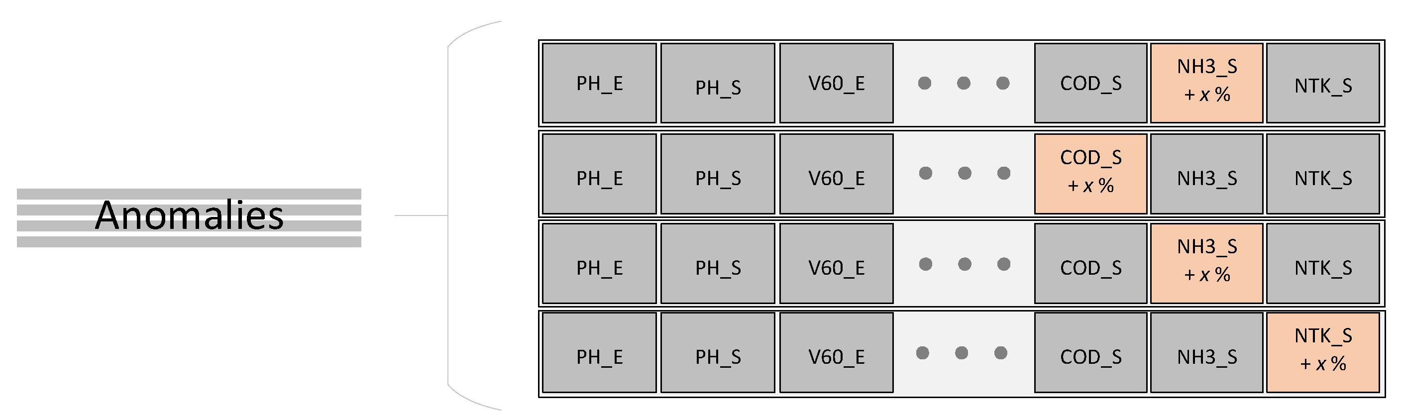
2.2. Unexpected Events Description

The present document deals with the detection of unexpected events in WWTPs that may represent a potential risk for final water quality. This offers help in managing undesired working situations, contributing to enhancement of optimum decision-making. However, given the unfeasibility of registering datasets in that kind of situation, a synthetic dataset is required to emulate anomalies. Different experts in the field of chemistry and water treatment were consulted to determine which variables are especially significant in detecting dangerous situations in a WWTP. Following these criteria, the output variables of Chemical Oxygen Demand (COD), Ammonia (NH3), and Total Kjeldahl Nitrogen (NTK) were identified as the most critical due to their relevance in assessing water quality and environmental impact. Specific reasons why these variables are essential in environmental and water treatment studies are described below.

• Chemical Oxygen Demand:

  –

  Organic Pollution Indicator: COD measures the amount of oxygen needed to oxidize organic matter in a water sample. It is a direct indicator of the amount of organic contaminants present [28].

  –

  Environmental Impact: High levels of COD in water bodies can result in decreased dissolved oxygen, affecting aquatic life and ecosystems [29].

  –

  Process Control: In wastewater treatment plants, COD is essential to monitor and control the efficiency of treatment processes [30].

• Ammonia:

  –

  Direct Toxicity: Ammonia is toxic to many aquatic species. Elevated levels can cause adverse effects in fish and other aquatic organisms [31].

  –

  Eutrophication: Ammonia is a nutrient that, in excess, can contribute to the eutrophication of water bodies, promoting extensive growth of algae and aquatic plants, which can lead to water quality degradation and the death of aquatic fauna by anoxia [32].

  –

  Pollution Indicator: The presence of ammonia can indicate recent contamination by agricultural, industrial, or domestic waste [33].

• Total Kjeldahl Nitrogen:

  –

  Total Nutrient Component: TKN measures the total amount of nitrogen in the form of ammonia and organic matter, providing a more complete view of the nitrogen load in water [34].

  –

  Eutrophication and Water Quality: Like ammonia, TKN is related to eutrophication. Excess nitrogen can promote the growth of oxygen-consuming organisms, degrading water quality and negatively affecting aquatic ecosystems [35].

  –

  Evaluation of Sources of Pollution: TKN helps to identify and quantify the sources of nitrogen pollution, whether agricultural, industrial, or urban [36].

In summary, these parameters are critical because they provide a comprehensive view of the pollutant load, potential toxicity, and environmental impact of water bodies. Their monitoring and control are essential for sustainable water resource management and protecting aquatic ecosystems. Hence, the generation of unexpected events followed the next steps:

• From the initial 237 samples, 16% were randomly selected to be converted to anomalies.
• For each instance selected, one of the three variables (COD_S, NH3_S, and NTK_S) was randomly selected.
• Once the variable to be modified was selected, its value was deviated by a given percentage.

Figure 2 represents the process of selecting random instances for anomaly generation. The original set is represented as a blue-colored square, and then, four random instances, represented in grey color, are converted to anomalies. The final set is divided into normal samples (target samples) and anomalous ones. Once the anomalous set is selected, Figure 3 represents the process to generate anomalies: one of the three key variables (COD_S, NH3_S, and NTK_S) is randomly selected, and its value is modified by a given percentage.

The final goal of this synthetic dataset is to determine situations that represent an emergency situation derived from abnormal values of critical variables such as COD_S, NH3_S, and NTK_S. Furthermore, the possibility of modifying the percentage x tested can provide an idea of classifier sensitivity.

2.3. One-Class Techniques

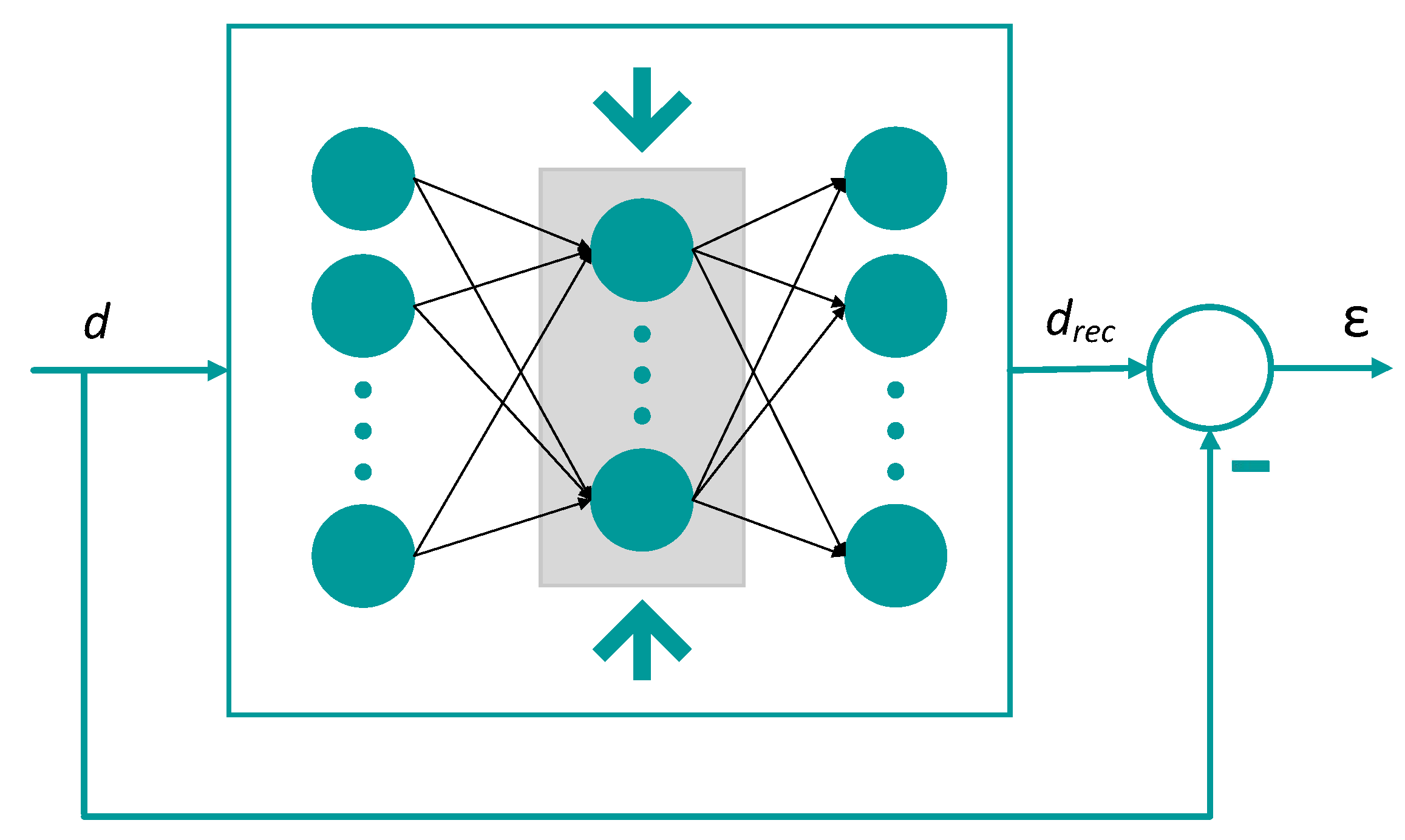
This paper proposes an intelligent classifier to detect risky situations in a WWTP. The proposal is based on learning the patterns of data registered only during normal operation. Once the model is trained, unexpected events can be determined if data differ from the learned patterns. Four different one-class techniques are proposed and described below to achieve this objective.

2.3.1. Autoencoder

This method utilizes an Autoencoder which relies on an Artificial Neural Network (ANN) to detect anomalies by determining their characteristics. Typically, the ANN setup includes an input layer, one or more hidden layers, and an output layer interconnected by weighted links [37]. The fundamental concept behind this approach involves reconstructing the input data (d) into output data ($d_{rec}$) through nonlinear dimensional reduction within the hidden layer, as depicted in Figure 4. Consequently, the number of neurons in the hidden layer is smaller than the input dimensions.

After the network undergoes training exclusively on the training dataset, data exhibiting distinct behaviors are expected to exhibit notable distinctions within the hidden layer space. Consequently, a test data point (q) is anticipated to demonstrate a substantial reconstruction error, quantified as $|d-d_{rec}|$. This metric serves as the criterion for categorizing the data as anomalous [38].

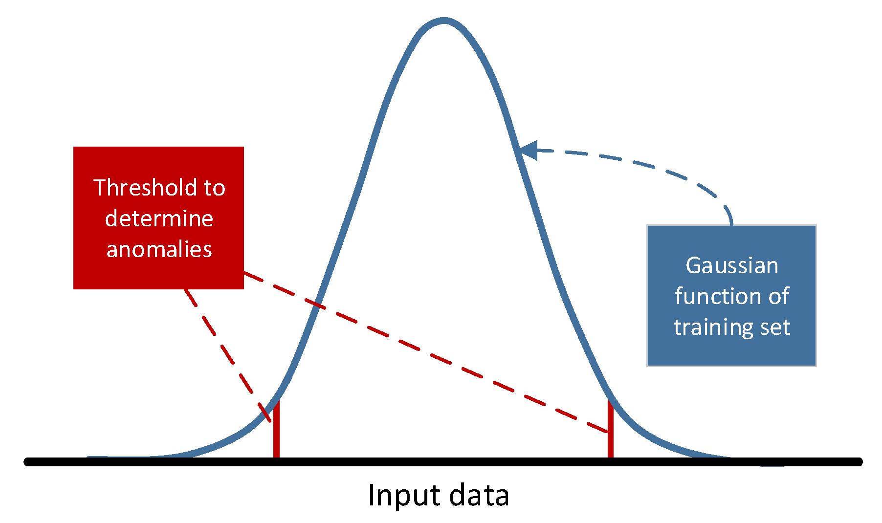
2.3.2. Gaussian Model

An alternative method for tackling anomaly detection, particularly in facial recognition, involves employing one-class techniques that rely on density functions. One straightforward approach within this paradigm is to apply a normal or Gaussian distribution function to the target dataset [38]. This function is derived from the same dataset used for training purposes.

After establishing the mean vector and covariance matrix, the method for identifying the anomalous status of a test sample relies on its evaluation within the Gaussian function. This straightforward approach offers a low computational overhead, making it advantageous, particularly for large datasets with a normal distribution shape.

In Figure 5, a simplified representation of a Gaussian function (depicted by the blue line) with a one-dimensional set is illustrated. The determination of whether a test instance is anomalous or not is based on comparing it to a predefined threshold (indicated by the red lines), which is set during the training phase.

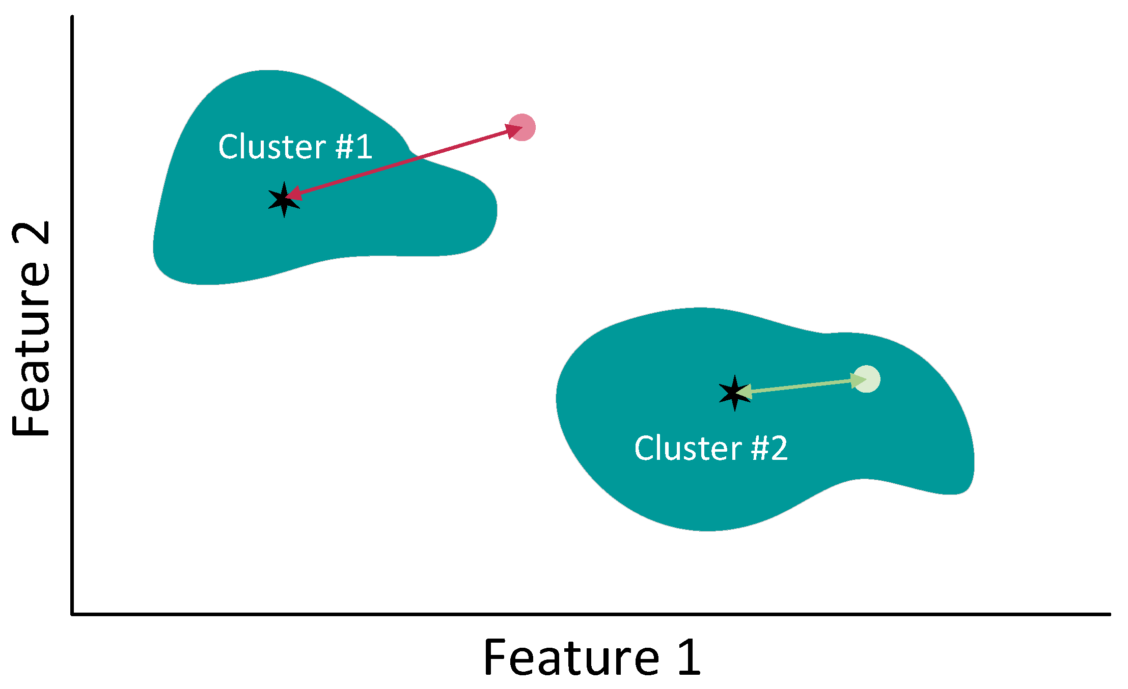
2.3.3. The K-means Algorithm

The K-means algorithm, an unsupervised technique widely employed in various domains like machine learning, image processing, and pattern recognition [39], aims to partition the dataset into clusters containing data points with similar characteristics [39].

Given a set $X=x_1,x_2,\dots ,x_N$, where $x_i\in {\mathbb{R}}^n$, the K-means algorithm partitions the data into K subsets $G_1,G_2,\dots ,G_K$, each associated with centroids $C=c_1,c_2,\dots ,c_K$, where $c_j\in {\mathbb{R}}^n$. This partitioning is performed based on a clustering error criterion [40], typically computed as the sum of Euclidean distances between each point $x_i\in {\mathbb{R}}^n$ and its centroid $c_j$.

The application of this algorithm using a one-class approach is based on the distance from test instances to their nearest centroid. It is considered anomalous if this value is greater than the maximum distance registered for that cluster during the training stage. Figure 6 shows an example in ${\mathbb{R}}^2$ where the training set is grouped into two clusters. Then, the green dot represents a test instance that is labeled as normal because the distance to its nearest centroid is below the maximum distance of that cluster. On the contrary, the long distance from the red dot to its centroid reveals the anomalous nature of the test instance.

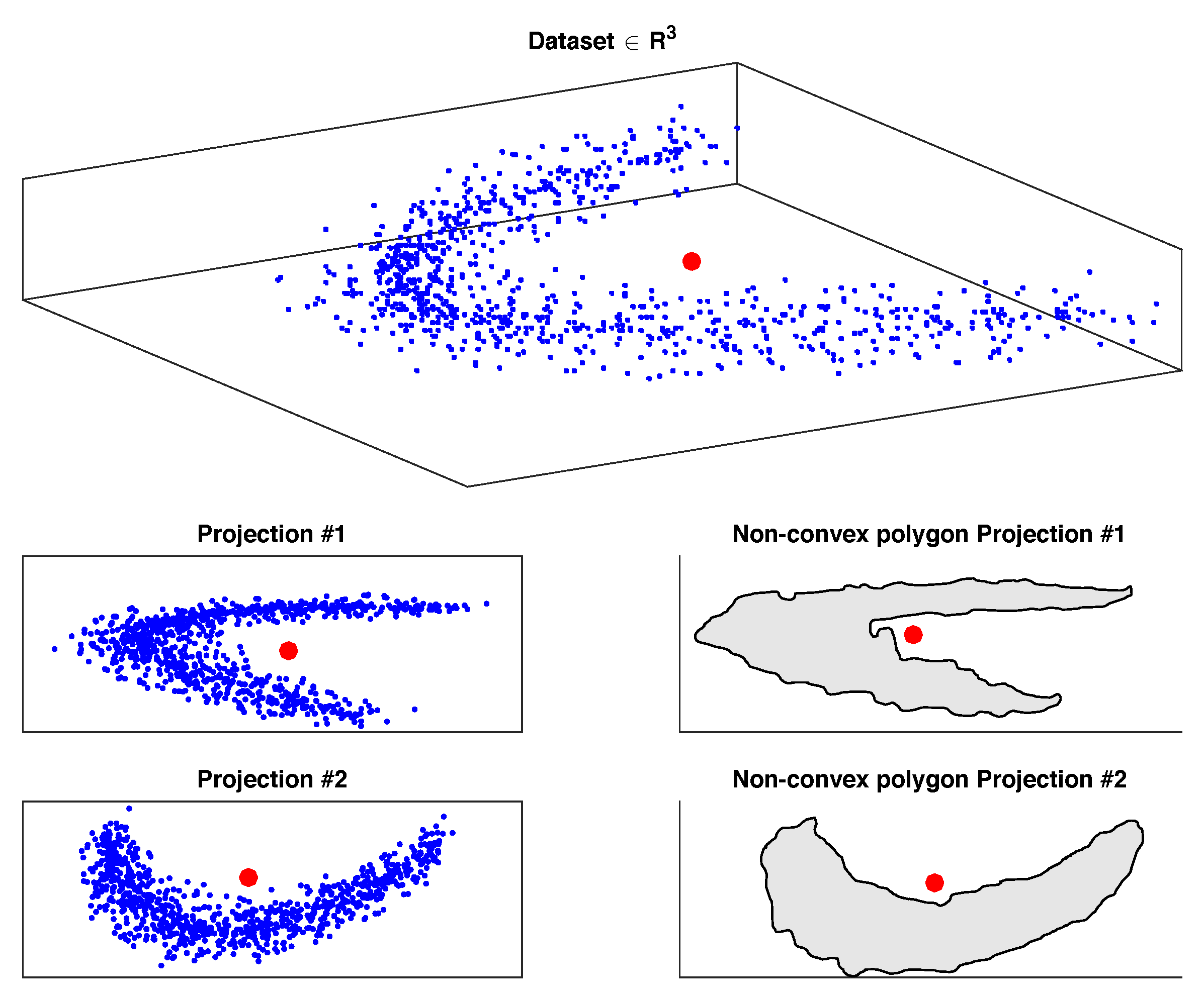
2.3.4. Non-Convex Boundary over Projections

The Non-Convex Boundary over Projections (NCBoP) algorithm innovatively utilizes non-convex hull calculations to model the shape of the target dataset [41]. This approach addresses limitations observed in the conventional convex hull method applied to random projections [42]. The fundamental principle of NCBoP involves approximating dataset boundaries in ${\mathbb{R}}^n$ by employing non-convex hulls across $\pi$ random projections onto 2D planes. Subsequently, non-convex limits are determined on these planes, thereby reducing the computational complexity associated with calculating non-convex limits across ${\mathbb{R}}^n$.

The NCBoP algorithm computes a non-convex polygon for each $\pi$ 2D random projection by initially selecting a starting point, determined as the lowest y coordinate among all points projected onto the $p_i$ plane. Subsequently, it identifies the K-nearest points and arranges them based on the polar angle, retaining only the furthest point from the starting point. This process is repeated for each 2D random projection.

After computing the initial points, a stack structure is established to accommodate the next third point. Subsequently, it evaluates whether the subsequent point in the list turns left (added to the stack) or right (removes the top point from the stack). This iterative process continues until it returns to the starting point. Once the training process concludes, all points are situated within the non-convex polygon generated by the algorithm.

Upon completion of the training phase, the criterion for identifying whether a new test point is anomalous is as follows: if the data fall outside of at least one of the t projected hulls, it is deemed anomalous. This determination is illustrated in Figure 7.

3. Experiments and Results

This section describes the different configurations considered for each one-class technique and the results derived from the proposed experiments.

3.1. Experiment Setup

As stated in previous sections, an initial dataset corresponding to normal working operations is used to train one-class classifiers. Then, unexpected and undesired data are introduced into those classifiers to determine whether they are capable of detecting hazardous situations. The severity of the anomalous event is checked with the aim of evaluating the classifier’s sensitivity. The percentage deviation is swept from 5 % to 95 % with a 10 % step. As no information about those anomalies is available during the training process, it is not feasible to apply feature selection techniques to evaluate the importance of each input variable in the classification process, so all variables are considered. In this sense, using an Autoencoder can contribute to reducing data dimension, compressing the data, and identifying sub-spaces with better performance.

To implement the best classifier for each type of anomaly, the experiments are configured according to the following parameters:

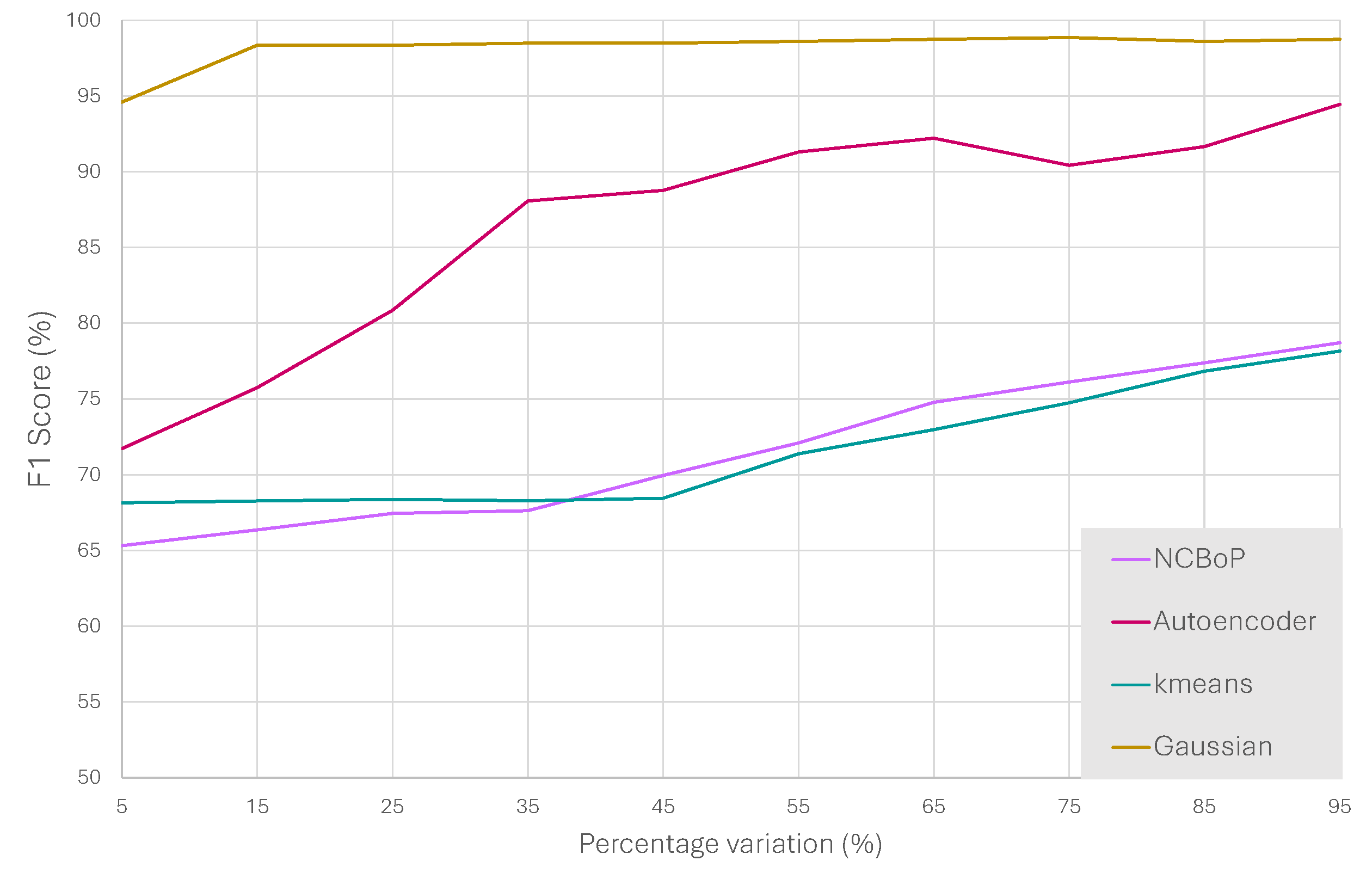
• Autoencoder: the input data of the neural network are comprised of the 23 variables monitored in the WWTP. The system is trained to learn the patterns from normal operation and replicate, at the output, the same value as the input. Once the model is trained, anomalous instances replicate the data at the output with significant error. This error, known as the reconstruction error, is the criteria to determine the anomaly detection. The number of layers is swept from 1 to 22, which is the number of variables minus one. The possibility of considering a percentage of anomalous points (OP) in the training set is checked: 0%, 5%, 10%, and 15%.
• Gaussian Model: the regularization parameter is swept from 0 to 0.005 with a step of 0.001. The possibility of considering a percentage of anomalous points (OPs) in the training set is checked: 0%, 5%, 10%, and 15%.
• K-means: the number of clusters is swept from 1 to 30. The possibility of considering a percentage of anomalous points (OPs) in the training set is checked: 0%, 5%, 10%, and 15%.
• NCBoP: the projections $\pi$ tested are 10, 50, 100, 500 and 1000. Furthermore, the $\lambda$ parameter in charge of reducing and expanding the boundaries is set to 0.6, 0.8, 1, 1.2, and 1.4.

All these configurations are tested through a five K-fold cross-validation process with three different data preparation methods: no preparation, Z-score, and 0–1 normalization. The mean values of the confusion matrix components during the five folds are registered. Furthermore, the F1-score parameter (%) is also included since it is an underscored metric in the field of anomaly detection, particularly in evaluating classifier ability to detect irregularities in complex systems [43,44]. To ensure classifier robustness, three aspects are taken into consideration:

• The instances converted to anomalies are randomly selected from the initial dataset.
• From each selected instance, the variable modified is also randomly selected.
• The process is repeated following K-fold cross-validation, ensuring that all data are subjected to both training and test phases.

3.2. Results

Autoencoder. The results achieved using Autoencoder classifiers are shown in

Table 2. Results and configuration for the best Autoencoder classifier depending on anomaly percentage deviation.

Dev (%)	Preproc	Hidden Layer	OP (%)	TP	TN	FP	FN	F1 (%)
5	Zscore	19	0	38.3	8.5	28.5	1.7	71.7
15	Zscore	20	5	34.2	20.9	16.1	5.8	75.7
25	Zscore	20	0	39.5	18.8	18.2	0.5	80.9
35	Zscore	20	5	34.3	33.4	3.6	5.7	88.1
45	Zscore	20	5	34	34.4	2.6	6	88.8
55	Zscore	18	5	34.1	36.4	0.6	5.9	91.3
65	Zscore	18	5	34.9	36.2	0.8	5.1	92.2
75	Zscore	20	5	34	35.8	1.2	6	90.4
85	Zscore	20	5	34.6	36.1	0.9	5.4	91.7
95	Zscore	18	5	35.8	37	0	4.2	94.5

. This technique shows a remarkable improvement in performance when the deviation percentage increases. In most cases, the best result corresponds to a configuration that considers 5% of the training set as anomalous. A common trend in all experiments consists of the use of a high number of neurons in the hidden layer, meaning that almost all variables are important to achieve the best classifier.

Gaussian Model. The Gaussian model results are shown in

Table 3. Results and configuration for best Gaussian classifier depending on anomaly percentage deviation.

Dev (%)	Preproc	RP	OP (%)	TP	TN	FP	FN	F1 (%)
5	Norm	0	5	35.9	37.0	0.0	4.1	94.6
15	Norm	0	0	38.7	37.0	0.0	1.3	98.3
25	Zscore	0	0	38.7	37.0	0.0	1.3	98.3
35	Norm	0	0	38.8	37.0	0.0	1.2	98.5
45	Zscore	0.001	0	38.8	37.0	0.0	1.2	98.5
55	Norm	0.001	0	38.9	37.0	0.0	1.1	98.6
65	Norm	0.001	0	39.0	37.0	0.0	1.0	98.7
75	Zscore	0.003	0	39.1	37.0	0.0	0.9	98.9
85	Zscore	0.003	0	38.9	37.0	0.0	1.1	98.6
95	Zscore	0.001	0	39.0	37.0	0.0	1.0	98.7

. This statistical technique leads to successful results with more than 95% of the F1-score in 9 out of 10 anomaly sets. The lowest value is achieved when the anomalies are generated by deviating only by 5% from the original value. In all cases, the anomalies are correctly classified (True Negative), with a really low number of situations in which a false alarm is set. In contrast to Autoencoder classifiers, an outlier percentage of 0% in the training set is the best possible configuration.

K-means. The results achieved using K-means classifiers are shown in

Table 4. Results and configuration for the best K-means classifier depending on anomaly percentage deviation.

Dev (%)	Preproc	OP (%)	k	TP	TN	FP	FN	F1 (%)
5	NoNorm	0	1	39.8	0.0	37.0	0.2	68.2
15	NoNorm	0	5	39.9	0.0	37.0	0.1	68.3
25	Zscore	0	3	40.0	0.0	37.0	0.0	68.4
35	Norm	0	29	39.4	1.0	36.0	0.6	68.3
45	Norm	0	12	39.7	0.7	36.3	0.3	68.4
55	Zscore	15	9	32.3	18.8	18.2	7.7	71.4
65	Zscore	10	9	34.3	17.3	19.7	5.7	73.0
75	Zscore	10	13	33.9	20.2	16.8	6.1	74.8
85	Zscore	10	17	33.0	24.1	12.9	7.0	76.8
95	Zscore	10	13	33.3	25.1	11.9	6.7	78.2

. Although the performance improves as the deviation increases, the F1 performance is below 80% in all cases, with consequent worse results than those of Autoencoder and Gaussian classifiers. The proper number of clusters to divide the dataset does not follow a common trend, varying from 1 to 29. The most critical aspect consists of the false positives that start with 37 (100% of the anomalies labeled as normal instances) and finish with 12, which is an improvable value.

NCBoP. 

Table 5. Results and configuration for best NCBoP classifier depending on anomaly percentage deviation.

Dev (%)	Preproc	$\mathit{\lambda }$	$\mathit{\pi }$	TP	TN	FP	FN	F1 (%)
5	NoNorm	0.8	500	37.1	0.5	36.5	2.9	65.3
15	Norm	1.4	10	36.5	3.5	33.5	3.5	66.4
25	Norm	1.4	10	37.7	2.9	34.1	2.3	67.4
35	Zscore	1.4	10	37.5	3.6	33.4	2.5	67.6
45	Zscore	1.4	100	30.5	20.3	16.7	9.5	70.0
55	Zscore	1.4	50	32.8	18.8	18.2	7.2	72.1
65	Zscore	1.2	10	33.2	21.4	15.6	6.8	74.8
75	Zscore	1.4	50	33.3	22.8	14.2	6.7	76.1
85	Zscore	1.4	100	31.3	27.4	9.6	8.7	77.4
95	Zscore	1.4	50	32.0	27.7	9.3	8.0	78.7

summarizes the performance of NCBoP classifiers in the different experiments. As in the case of K-means, the F1-score does not exceed 80% in any configuration with a great number of anomalous instances classified as normal. The value of $\lambda$ is 1.4 in 8 out of 10 cases, which means that an increment in the decision boundary leads to better results. However, when the deviation used to generate the anomaly is 5%, the decision boundary should be reduced. The number of projections does not follow a recognizable pattern, varying depending on the experiment.

To understand the improvement of each algorithm with the percentage variation of COD_S, NH3_S, and NTK_S, Figure 8 represents the values of the F1-score for each technique. The Gaussian model approach is the best algorithm to detect test parameter deviations.

4. Discussion

The presented work proposed a semi-supervised methodology to detect alarm situation in a WWTP. The importance of the proposal lies on the fact of implementing classifiers that take into consideration all system variables registered from normal operation with no need of human expertise to determine unexpected and anomalous events. In the current context of digitalization and quality standard increment, this tool takes advantage of data availability to enhance the supervision and diagnostics in critical infrastructure. The proposal can complement traditional diagnosis and supervision systems, offering an alarm in case of early anomaly detection. This contributes to maintenance decision making, easing effectiveness, and economic and energy efficiency. Furthermore, the results show how classifier performance improves significantly when the deviation is greater, resulting in a more dangerous situation. Despite the clear advantages of the proposal, there are several factors to which a one-class approach cannot contribute. As this is a semi-supervised methodology, it is necessary to have an initial set of normal operation instances, so human expertise is needed at least during the first data registration stage to ensure data quality. Once this limitation is overcome, the combination of the proposal with other supervised techniques will be suitable for detecting sensor misreadings to complement the one-class classifier.

5. Conclusions and Future Works

This paper presents the use of different one-class techniques to determine the appearance of unexpected events in a WWTP facility. Those events are synthetically generated to simulate deviations in COD_S, NH3_S, and NTK_S, representing critical measures to determine potential risks. With the aim of evaluating how effective each technique is, the tested deviations varied from 5% to 95%. In general terms, an increase in that deviation results in better performance in four techniques. Although NCBoP, K-means, and Autoencoder present a remarkable improvement with each deviation step, Gaussian classifiers achieve the best results. The experiments and results for the technique showed that, after a five K-fold validation, all negative instances (unexpected and hence undesired events) were correctly labeled. The false alarm cases were significantly low, with a mean value below 1.5 samples in all experiments above 15% deviation.

The results indicated that the proposed system represents a valuable contribution to the WWTP monitoring process. Taking into consideration the 23 variables along the facility, it is possible to detect when three critical parameters present unexpected values, according to the patterns learned from normal operation sets.

In future works, there are three alternative ways to supplement the contribution. The first would consider individual classifiers for each tested parameter: COD_S, NH3_S, and NTK_S. Although the classified proposed detects all unexpected events with the Gaussian model, this approach could improve the rest of the classifiers. Furthermore, instead of semi-supervised algorithms in which only information from normal operation is available, the use of supervised classifiers could be tested. This approach would implement a classifier for normal operation and another one for unexpected deviation. In the case of good results, these classifiers would indicate the specific parameter with unexpected performance. Finally, it could be possible to consider the modification of other variable instead of COD_S, NH3_S, and NTK_S to detect an unexpected situation that correspond to less severe scenarios.

References

1. Şenol, R.; Salman, O.; Kaya, Z. Potable water production from ambient moisture. Appl. Water Sci. 2023, 13, 10. [Google Scholar] [CrossRef]
2. Brown, T.C.; Mahat, V.; Ramirez, J.A. Adaptation to future water shortages in the United States caused by population growth and climate change. Earth’s Future 2019, 7, 219–234. [Google Scholar] [CrossRef]
3. Boretti, A.; Rosa, L. Reassessing the projections of the world water development report. NPJ Clean Water 2019, 2, 15. [Google Scholar] [CrossRef]
4. Safarpour, H.; Tabesh, M.; Shahangian, S.A. Environmental Assessment of a Wastewater System under Water demand management policies. Water Resour. Manag. 2022, 36, 2061–2077. [Google Scholar] [CrossRef]
5. Spellman, F.R. Handbook of Water and Wastewater Treatment Plant Operations; CRC Press: Boca Raton, FL, USA, 2013. [Google Scholar]
6. Mascher, F.; Mascher, W.; Pichler-Semmelrock, F.; Reinthaler, F.F.; Zarfel, G.E.; Kittinger, C. Impact of Combined Sewer Overflow on Wastewater Treatment and Microbiological Quality of Rivers for Recreation. Water 2017, 9, 906. [Google Scholar] [CrossRef]
7. Ianes, J.; Cantoni, B.; Remigi, E.U.; Polesel, F.; Vezzaro, L.; Antonelli, M. A stochastic approach for assessing the chronic environmental risk generated by wet-weather events from integrated urban wastewater systems. Environ. Sci. Water Res. Technol. 2023, 9, 3174–3190. [Google Scholar] [CrossRef]
8. Lu, J.Y.; Wang, X.M.; Liu, H.Q.; Yu, H.Q.; Li, W.W. Optimizing operation of municipal wastewater treatment plants in China: The remaining barriers and future implications. Environ. Int. 2019, 129, 273–278. [Google Scholar] [CrossRef] [PubMed]
9. Bertanza, G.; Boiocchi, R.; Pedrazzani, R. Improving the quality of wastewater treatment plant monitoring by adopting proper sampling strategies and data processing criteria. Sci. Total Environ. 2022, 806, 150724. [Google Scholar] [CrossRef] [PubMed]
10. Longo, S.; d’Antoni, B.M.; Bongards, M.; Chaparro, A.; Cronrath, A.; Fatone, F.; Lema, J.M.; Mauricio-Iglesias, M.; Soares, A.; Hospido, A. Monitoring and diagnosis of energy consumption in wastewater treatment plants. A state of the art and proposals for improvement. Appl. Energy 2016, 179, 1251–1268. [Google Scholar] [CrossRef]
11. Martínez, R.; Vela, N.; el Aatik, A.; Murray, E.; Roche, P.; Navarro, J.M. On the Use of an IoT Integrated System for Water Quality Monitoring and Management in Wastewater Treatment Plants. Water 2020, 12, 1096. [Google Scholar] [CrossRef]
12. Kizgin, A.; Schmidt, D.; Joss, A.; Hollender, J.; Morgenroth, E.; Kienle, C.; Langer, M. Application of biological early warning systems in wastewater treatment plants: Introducing a promising approach to monitor changing wastewater composition. J. Environ. Manag. 2023, 347, 119001. [Google Scholar] [CrossRef] [PubMed]
13. Bagherzadeh, F.; Mehrani, M.J.; Basirifard, M.; Roostaei, J. Comparative study on total nitrogen prediction in wastewater treatment plant and effect of various feature selection methods on machine learning algorithms performance. J. Water Process Eng. 2021, 41, 102033. [Google Scholar] [CrossRef]
14. Ye, G.; Wan, J.; Deng, Z.; Wang, Y.; Chen, J.; Zhu, B.; Ji, S. Prediction of effluent total nitrogen and energy consumption in wastewater treatment plants: Bayesian optimization machine learning methods. Bioresour. Technol. 2024, 395, 130361. [Google Scholar] [CrossRef] [PubMed]
15. Murei, A.; Kamika, I.; Momba, M.N.B. Selection of a diagnostic tool for microbial water quality monitoring and management of faecal contamination of water sources in rural communities. Sci. Total Environ. 2024, 906, 167484. [Google Scholar] [CrossRef]
16. Borzooei, S.; Campo, G.; Cerutti, A.; Meucci, L.; Panepinto, D.; Ravina, M.; Riggio, V.; Ruffino, B.; Scibilia, G.; Zanetti, M. Optimization of the wastewater treatment plant: From energy saving to environmental impact mitigation. Sci. Total Environ. 2019, 691, 1182–1189. [Google Scholar] [CrossRef]
17. Muoio, R.; Palli, L.; Ducci, I.; Coppini, E.; Bettazzi, E.; Daddi, D.; Fibbi, D.; Gori, R. Optimization of a large industrial wastewater treatment plant using a modeling approach: A case study. J. Environ. Manag. 2019, 249, 109436. [Google Scholar] [CrossRef]
18. Cunha, D.L.; da Silva, A.S.; Coutinho, R.; Marques, M. Optimization of ozonation process to remove psychoactive drugs from two municipal wastewater treatment plants. Water Air Soil Pollut. 2022, 233, 67. [Google Scholar] [CrossRef]
19. Garcia-Alvarez, D.; Fuente, M.; Vega, P.; Sainz, G. Fault Detection and Diagnosis using Multivariate Statistical Techniques in a Wastewater Treatment Plant.* *This work was supported in part by the national research agency of Spain (CICYT) through the project DPI2006-15716-C02-02 and the regional government of Castilla y Leon through the project VA052A07. IFAC Proc. Vol. 2009, 42, 952–957. [Google Scholar] [CrossRef]
20. Corominas, L.; Villez, K.; Aguado, D.; Rieger, L.; Rosén, C.; Vanrolleghem, P.A. Performance evaluation of fault detection methods for wastewater treatment processes. Biotechnol. Bioeng. 2011, 108, 333–344. [Google Scholar] [CrossRef]
21. Schraa, O.; Tole, B.; Copp, J.B. Fault detection for control of wastewater treatment plants. Water Sci. Technol. 2006, 53, 375–382. [Google Scholar] [CrossRef]
22. Ruiz, M.; Sin, G.; Berjaga, X.; Colprim, J.; Puig, S.; Colomer, J. Multivariate Principal Component Analysis and Case-Based Reasoning for monitoring, fault detection and diagnosis in a WWTP. Water Sci. Technol. 2011, 64, 1661–1667. [Google Scholar] [CrossRef] [PubMed]
23. Carballo Mato, J.; González Vázquez, S.; Fernández Águila, J.; Delgado Rodríguez, A.; Lin, X.; Garabato Gándara, L.; Sobreira Seoane, J.; Silva Castro, J. Foam Segmentation in Wastewater Treatment Plants. Water 2024, 16, 390. [Google Scholar] [CrossRef]
24. Lin, H.; Lin, C.; Xie, D.; Acuna, P.; Liu, W. A Counter-Based Open-Circuit Switch Fault Diagnostic Method for a Single-Phase Cascaded H-Bridge Multilevel Converter. IEEE Trans. Power Electron. 2023, 39, 814–825. [Google Scholar] [CrossRef]
25. Lin, H.; Cai, C.; Chen, J.; Gao, Y.; Vazquez, S.; Li, Y. Modulation and control independent dead-zone compensation for H-bridge converters: A simplified digital logic scheme. IEEE Trans. Ind. Electron. 2024, 1–6. [Google Scholar] [CrossRef]
26. Orhon, D. Evolution of the activated sludge process: The first 50 years. J. Chem. Technol. Biotechnol. 2014, 90, 608–640. [Google Scholar] [CrossRef]
27. Matamoros, V.; Salvadó, V. Evaluation of a coagulation/flocculation-lamellar clarifier and filtration-UV-chlorination reactor for removing emerging contaminants at full-scale wastewater treatment plants in Spain. J. Environ. Manag. 2013, 117, 96–102. [Google Scholar] [CrossRef] [PubMed]
28. Eddy, M.; Abu-Orf, M.; Bowden, G.; Burton, F.L.; Pfrang, W.; Stensel, H.D.; Tchobanoglous, G.; Tsuchihashi, R.; Firm, A. Wastewater Engineering: Treatment and Resource Recovery; McGraw Hill Education: New York, NY, USA, 2014. [Google Scholar]
29. Sawyer, C.N.; McCarty, P.L.; Parkin, G.F. Chemistry for Environmental Engineering and Science; McGraw-Hill: New York, NY, USA, 2003. [Google Scholar]
30. Tchobanoglus, G.; Burton, F.; Stensel, H.D. Wastewater engineering: Treatment and reuse. Am. Water Work. Assoc. J. 2003, 95, 201. [Google Scholar]
31. Huff, L.; Delos, C.; Gallagher, K.; Beaman, J. Aquatic Life Ambient Water Quality Criteria for Ammonia-Freshwater; US Environmental Protection Agency: Washington, DC, USA, 2013. [Google Scholar]
32. Carpenter, S.R.; Caraco, N.F.; Correll, D.L.; Howarth, R.W.; Sharpley, A.N.; Smith, V.H. Nonpoint pollution of surface waters with phosphorus and nitrogen. Ecol. Appl. 1998, 8, 559–568. [Google Scholar] [CrossRef]
33. World Health Organization. Ammonia in Drinking-Water: Background Document for Development of WHO Guidelines for Drinking-Water Quality. WHO. 2003. Available online: https://cdn.who.int/media/docs/default-source/wash-documents/wash-chemicals/ammonia.pdf?sfvrsn=3080badd_6 (accessed on 12 June 2024).
34. Holmes, D.E.; Dang, Y.; Smith, J.A. Nitrogen cycling during wastewater treatment. Adv. Appl. Microbiol. 2019, 106, 113–192. [Google Scholar]
35. Smith, V.H.; Tilman, G.D.; Nekola, J.C. Eutrophication: Impacts of excess nutrient inputs on freshwater, marine, and terrestrial ecosystems. Environ. Pollut. 1999, 100, 179–196. [Google Scholar] [CrossRef]
36. Camargo, J.A.; Alonso, Á. Ecological and toxicological effects of inorganic nitrogen pollution in aquatic ecosystems: A global assessment. Environ. Int. 2006, 32, 831–849. [Google Scholar] [CrossRef] [PubMed]
37. Sakurada, M.; Yairi, T. Anomaly detection using autoencoders with nonlinear dimensionality reduction. In Proceedings of the MLSDA 2014 2nd Workshop on Machine Learning for Sensory Data Analysis, New York, NY, USA, 2 December 2014; p. 4. [Google Scholar]
38. Tax, D.M.J. One-Class Classification: Concept-Learning in the Absence of Counter-Examples. Ph.D. Thesis, Delft University of Technology, Delft, The Netherlands, 2001. [Google Scholar]
39. Ahmed, M.; Seraj, R.; Islam, S.M.S. The k-means algorithm: A comprehensive survey and performance evaluation. Electronics 2020, 9, 1295. [Google Scholar] [CrossRef]
40. Chong, B. K-means clustering algorithm: A brief review. Acad. J. Comput. Inf. Sci. 2021, 4, 37–40. [Google Scholar]
41. Jove, E.; Casteleiro-Roca, J.L.; Quintián, H.; Méndez-Pérez, J.A.; Calvo-Rolle, J.L. A new method for anomaly detection based on non-convex boundaries with random two-dimensional projections. Inf. Fusion 2021, 65, 50–57. [Google Scholar] [CrossRef]
42. Sartipizadeh, H.; Vincent, T.L. Computing the approximate convex hull in high dimensions. arXiv 2016, arXiv:1603.04422. [Google Scholar]
43. Zakariah, M.; Almazyad, A.S. Anomaly Detection for IOT Systems Using Active Learning. Appl. Sci. 2023, 13, 12029. [Google Scholar] [CrossRef]
44. Almotairi, A.; Atawneh, S.; Khashan, O.A.; Khafajah, N.M. Enhancing intrusion detection in IoT networks using machine learning-based feature selection and ensemble models. Syst. Sci. Control Eng. 2024, 12, 2321381. [Google Scholar] [CrossRef]
Figure 1. Scheme of the operation of the WWTP under study.
Applsci 14 05185 g001
Figure 2. Random selection of instances for anomaly generation.
Applsci 14 05185 g002
Figure 3. Procedure of generation of anomalies.
Applsci 14 05185 g003
Figure 4. Cluster division depending on the value of K.
Applsci 14 05185 g004
Figure 5. Example of Gaussian Model for one-class task in R 1 .
Applsci 14 05185 g005
Figure 6. An example of a K-means algorithm applied to anomaly detection in 2D.
Applsci 14 05185 g006
Figure 7. Example of NCBoP for one-class techniques in R 3 .
Applsci 14 05185 g007
Figure 8. F1-score for each classifer.
Applsci 14 05185 g008