Abstract
One of the goals of developing and implementing Industry 4.0 solutions is to significantly increase the level of flexibility and autonomy of production systems. It is intended to provide the possibility of self-reconfiguration of systems to create more efficient and adaptive manufacturing processes. Achieving such goals requires the comprehensive integration of digital technologies with real production processes towards the creation of the so-called Cyber–Physical Production Systems (CPPSs). Their architecture is based on physical and cybernetic elements, with a digital twin as the central element of the “cyber” layer. However, for the responses obtained from the cyber layer, to allow for a quick response to changes in the environment of the production system, its virtual counterpart must be supplemented with advanced analytical modules. This paper proposes the method of creating a digital twin production system based on discrete simulation models integrated with deep reinforcement learning (DRL) techniques for CPPSs. Here, the digital twin is the environment with which the reinforcement learning agent communicates to find a strategy for allocating processes to production resources. Asynchronous Advantage Actor–Critic and Proximal Policy Optimization algorithms were selected for this research.
1. Introduction
The implementation of Industry 4.0 solutions, currently observed in various branches of the manufacturing industry, is expected to result in a transition from traditional production systems to smart, more flexible, autonomous, and reconfigurable cyber–physical systems. It is related to the transition from intelligent production based on knowledge to smart production based on data and knowledge, where the term “smart” refers to the creation, acquisition, and use of data, which use both advanced information and communication technologies, as well as advanced data analysis. As a result, future production systems and their management methods will be supported by real-time data transmission, exchange, and analysis technologies along with simulation and optimization based on digital models [1,2,3]. Scientific and industrial research in this area is supported by developing key technologies related to the concept of Industry 4.0, such as the Internet of Things, big data, cloud computing, Embedded Systems, and artificial intelligence. The creation of a communication interface between the digital and physical world through the integration of computations, networks, and physical resources is called cyber–physical systems (CPSs), and, concerning production systems, Cyber–Physical Production Systems (CPPSs) [2,4,5]. Apart from physical elements, a cyber–physical system is characterized by a cyber layer, the main element of which is a virtual component—a digital twin (DT) of the production system. DTs are taking a central position in new-generation intelligent production through integration with a CPPS, and their architecture should allow simultaneous access to production data and their processing [5,6]. A CPS, therefore, is a system that aggregates available information to predict conditions in production plants and demonstrates the advantages of additional optimization through data collection, analysis, and processing, and also helps to make decisions through control or prediction [7,8,9].
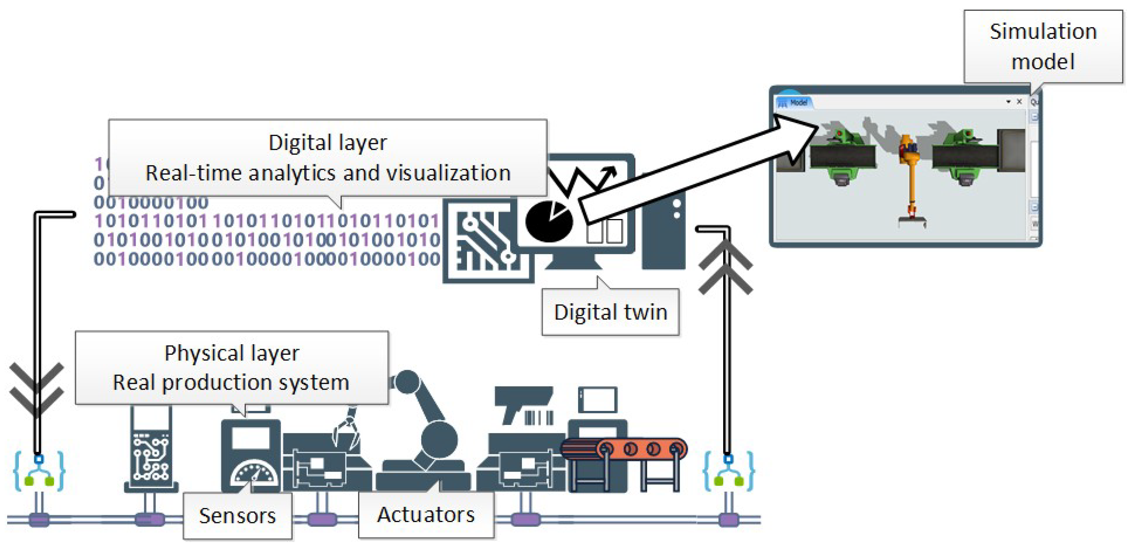
In this context, the search for easily industrially applicable and effective methods for creating DTs is particularly topical. It is a challenge currently faced by researchers and engineers of production systems. As recent research shows, the creation of digital twins, which are the central element of a CPPS, can be successfully implemented using discrete-event computer simulation models [10,11,12,13,14]. The very concept of a twin, in the sense of a prototype/copy of an existing object that mirrors actual operating conditions in order to simulate its behavior in real time, appeared during NASA’s Apollo program [15]. Since then, computer simulation methods and tools have undergone a process of continuous development, passing through phases from individual applications of simulation models to supporting the solution of specific problems and areas through simulation-based system design support, today’s digital twin concepts, where simulation models constitute the center of the functionality of the CPS [14,15]. A simplified view of the system architecture is shown in Figure 1.
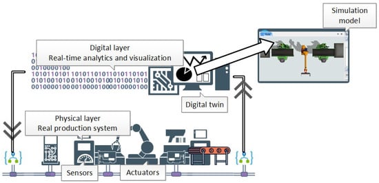
Figure 1.
Cyber–physical system and a simulation model as a digital twin.
The approaches to using simulation models as a DT proposed in the literature, including, in particular, the references indicated above, obviously differ in scope and functionality, both with respect to the model itself and the scope and direction of data exchange between data sources and the simulation model. Depending on the possibility of updating the state of the simulation model objects and the direction of data exchange in [16], the authors divided digital mappings into three categories of digital representation of physical objects (a classification of digital twins):
- Digital Model—which does not use any form of automatic data integration between the physical object and the digital object;
- Digital Shadow—in which there is an automated one-way flow of data between the state of a physical and digital object;
- Digital Twin—where data flows (in both directions) between the existing physical and digital objects are fully integrated.
Of course, in the applications of simulation models described above, since the DT is the central element of the CPPS, the DT should have the functionality of the third category. The possibility of bi-directional communication along with the mapping and simulation of the behavior, functioning, and performance of the physical counterpart are only necessary conditions that allow their use as the main element of the cyber layer. For digital twins to become useful in supporting decision-making in the areas of planning and control of physical system objects, it is necessary to enrich the cyber layer (or the digital twin itself) with analytical modules that allow for the determination of solutions that can be sent to the control system in real time. The challenges faced by such solutions correspond to the requirements of the third and fourth levels of development of production management and control strategies in the four-level development scale proposed by Zhuang, Liu and Xiong [17] concerning manufacturing systems (Figure 2). The first level of development is characterized by the so-called passive (reactive) management and control methods, where most of the data are collected and entered offline, and traditional relational databases can meet most data management requirements. At the next stage, data are collected in real time using RFID tags, sensors, and barcodes, and are transmitted over real-time networks, enabling faster data processing and decision-making. The third and fourth stages ensure the use of appropriately predictive and proactive management and control methods. They will require extensive machine learning applications, artificial intelligence methods, cloud computing, and other big data technologies.
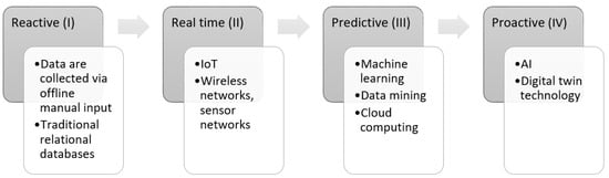
Figure 2.
Development of production management and control strategies.
The predictive strategy is to be based on combined big data and digital twin technologies. In the case of a proactive strategy, it may even be possible to control physical systems based on the self-adaptation and self-reconfiguration functions of the CPPS. It is an extension of the predictive strategy towards intelligent management and production control, thanks to the combination of artificial intelligence technologies and digital twins. Currently, many companies are still at the first or second stage of development [17]. Similarly, the Digital Twin-based Manufacturing System (DTMS) model proposed in [18] is a novel reference emphasizing fusion, interaction, and iteration. Regarding iteration, the system continuously analyzes the production process and continuously iteratively corrects the DT model to improve the overall DTMS. The authors in [18] point out that the manufacturing industry is currently in an era of rapid and intelligent development thanks to the strengthening of information technologies. In this context, the research on DTMS has become a “hot topic” in both academic and industrial circles.
The need to respond to changing environmental factors and to autonomously reconfigure the production system or adapt to these changes indicated above in relation to the Industry 4.0 concept highlights the great potential of machine learning applications and the ability to achieve promising results in the field of production research. Moreover, it is pointed out that classical methods of allocating processes to resources, based on priority dispatching rules or evolutionary algorithms, are not adapted to the dynamic environment in modern production [19,20]. It becomes necessary to enrich CPPSs with solutions, e.g., implementing advanced artificial intelligence and machine learning methods. In such a combination, the DT reflecting the behavior of the production system can play the role of a virtual environment used in the training phase. It is especially important in relation to today’s requirements, where companies have to deal with mass customization, complex technologies, and shortening product life cycles. They must, therefore, be able to operate under highly dynamic market conditions and meet increasing sustainability standards. In recent years, there has been a significant increase in interest in the use of reinforcement learning algorithms, and also in the area of production systems [19].
Regardless of the production planning or control problem considered, the architectures of RL agent interaction in the training process proposed in the literature indicate the need to develop an environment (appropriate for a given problem and system) in which the Deep RL agent can interact. Most non-simulation-based approaches to solving production planning problems use analytical models. These models often describe a problem through the objective function, as well as constraints to define the problem’s structure [21]. Developing analytical models of real production planning, scheduling, and sequencing problems are complex tasks [21]. Analytical models are now often the basis for modules that determine, for example, the production schedule and production indicators and, as a result, the value of the reward function in the communication process with the RL agent [22,23,24,25]. In many cases, the interaction environment is based on dedicated computational algorithms and mathematical models, where it is necessary to develop formulas that calculate subsequent states and rewards based on the state and action (see, e.g., [22,26,27,28,29]).
However, compared to the DT based on discrete simulation models considered in this paper, modifying analytical models, especially related to adding a new type of constraint or combining models covering different subsystems or production planning areas, is usually also a complex and time-consuming task. The DT, thanks to the direct access to operational data and the use of communication techniques for data acquisition, allows a fast semi-automatic or automatic adaptation of the simulation model. In addition, 3D simulation models also take into account intralogistics subsystems and/or the availability of operators and their travel times, which are usually omitted in dedicated analytical models. They can be quickly adapted to changes resulting from emergencies that require route changes and the use of alternative resources, supply chain disruptions at various levels, and changes in demand. This also meets the requirements of the latest concepts of the so-called Symbiotic Simulation System [30]. Analytical approaches, due to the need to update mathematical models and formulas (the agent’s interaction environment) in the event of changes (often even minor ones) in the real production system, may be too inflexible in practical industrial applications.
This gap motivated research in the area of using DTs of production systems based on modern computer discrete simulation systems as an environment for the interaction of reinforced machine learning agents, the results of which are presented in this paper. Additionally, many studies provide the parameters of the RL algorithms used (e.g., [31]). Still, there is no analysis or discussion of the impact of their values on the results obtained or the speed of the training process. The results of such analyses may assist in their selection in future studies and show areas of possible shortening of responses by shortening the training time.
The highlights and contributions of this paper are as follows: (1) the proposed CPPS architecture for solving the DRL agent learning process, in which the agent communicates with the production system digital twin, so that the agent does not have to interact with the real workshop environment; (2) an example of the practical implementation of DRL algorithms in solving manufacturing process allocation problems along with a comparison of the effectiveness of selected algorithms, and results and conclusions from the analysis of the impact of selected DRL algorithms parameters’ values on the quality of the found policy models and training speed.
In the following section, the basics of RL, an overview of selected RL algorithms, and related work are presented. In Section 3, the proposed CPPS architecture for solving the DRL agent training process is described. The comparison experiments are implemented in Section 4. Section 5 discusses the results. The last section contains short conclusions and areas of further research work.
2. Reinforcement Learning
Reinforcement learning (RL) is a subcategory of machine learning and differs from supervised and unsupervised learning in particular by its trial-and-error approach to learning in direct interaction with the environment [19,32]. Reinforcement learning was previously identified as one of the breakthrough technologies by MIT Technology Review [33] as a technology with great potential in a wide range of applications [19]. It is indicated that it may revolutionize the field of artificial intelligence and will play a key role in its future achievements. RL is also part of the ongoing trend in artificial intelligence and machine learning towards greater integration with statistics and optimization [32].
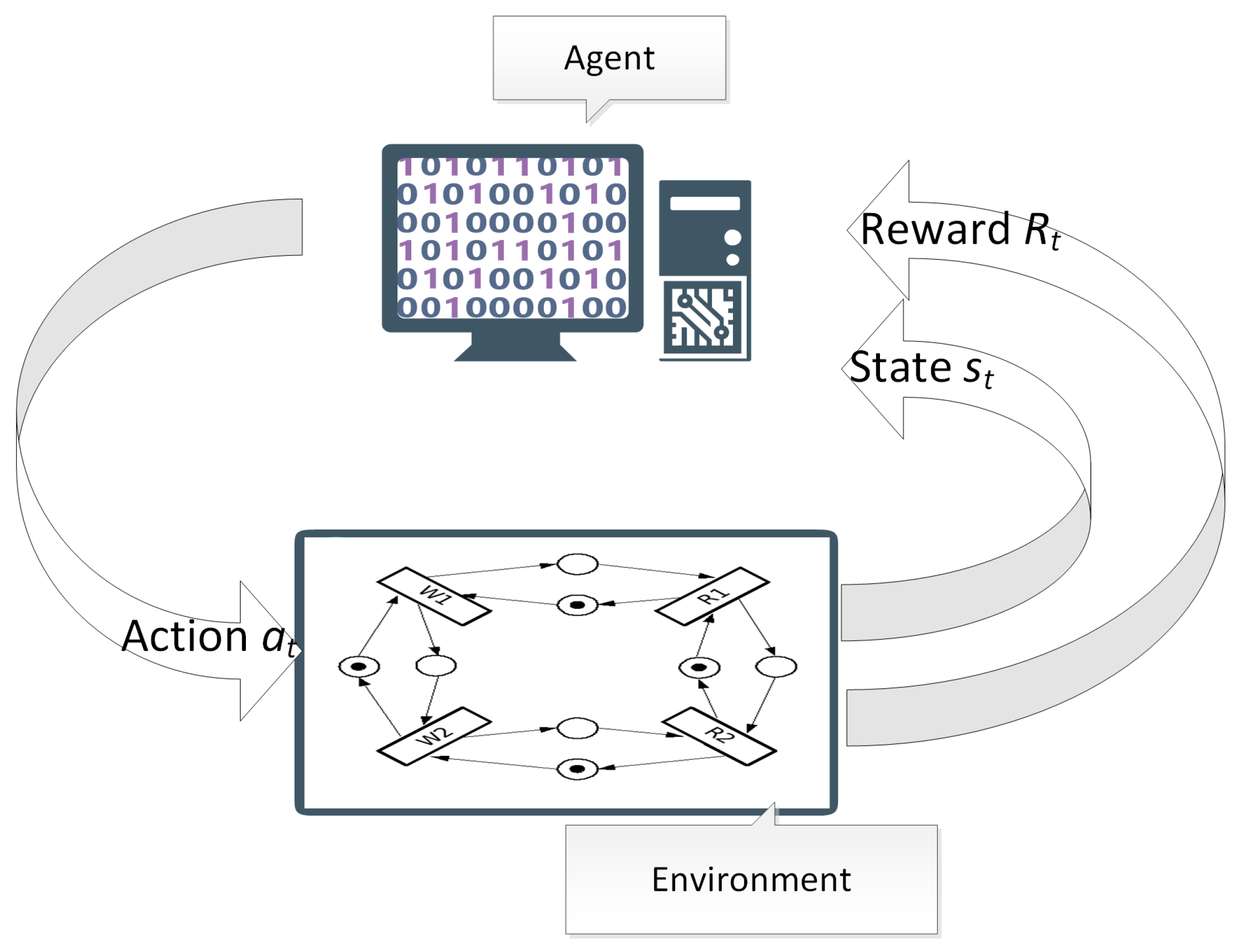
Formally, the problem of reinforcement learning uses the ideas of dynamic systems theory. In particular, optimal control of the Markov decision-making process provides mathematical frameworks to model decision-making under uncertainty. The basic idea is to capture aspects of the real problem that the learning agent is supposed to solve by interacting with the environment and taking actions that affect the state of the environment in order to achieve the set goal [32]. An autonomous agent controlled by an RL algorithm observes and receives a state from the environment (at time step t). Then, it interacts with the environment and executes an action according to its policy . The policy is also known as an agent strategy. After acting, the environment transits to a new state based on the current state and action, and provides an immediate reward to the agent [34,35] (Figure 3). The reward can be positive or negative—positive is awarded in exchange for successful actions, and negative represents penalties.
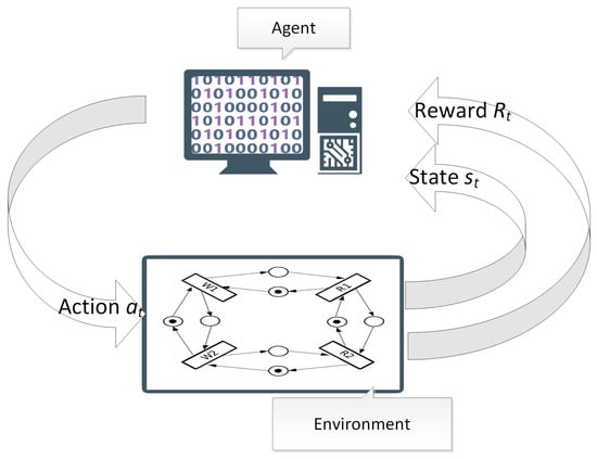
Figure 3.
Reinforcement learning—environment and agent interaction concept.
RL is another machine learning paradigm alongside supervised and unsupervised learning. RL differs from supervised learning, in which learning occurs from an external training set of tagged examples for solving a given problem class. Its goal is, among other things, extrapolation by the system of its answers so that it works correctly in situations not present in the training set [32]. For this reason, supervised learning is not practical in solving dynamic interactive problems for which we cannot even prepare a training set, representative for all situations we do not know. An example of such environments is production systems operating in changing environmental conditions, in which the agent must be able to learn from its own experience. RL also differs from the other current machine learning paradigm, unsupervised learning. Despite the apparent similarities between RL and unsupervised learning, which also does not rely on examples of correct behavior (training set), the main difference is that RL is looking for a way to maximize reward value rather than looking for a hidden structure. With regard to RL, unlike many other approaches that address subproblems without dealing with how they might fit into the bigger picture [32], a key feature that makes RL suitable for solving production management problems is that RL takes into account the whole problem of a goal-oriented agent interacting with an unknown, changing environment.
The rapid development and a significant increase in interest in RL algorithms are also related to the development of deep learning in recent years, based on the function approximation and powerful representation capabilities of deep neural networks. The advent of deep learning has had a significant impact on many areas of machine learning, improving the state of the art. In particular, deep reinforcement learning (DRL) combines both a deep learning architecture with a reinforcement learning architecture to perform a wide range of complex decision-making tasks that were previously infeasible for a machine. DRL in machine learning practice allowed to solve previous problems related to the lack of scalability, limitations to fairly small-dimensional problems, or dimensionality problems (memory complexity, computational complexity, and sample complexity) [35]. More information and explanations about DRL technology in machine learning can be found, i.e., in [19,32,36]. RL algorithms based on these methods have become very popular in recent years [32].
To update a learning agent’s way of behavior, the agent needs a learning algorithm. Given an optimal system, the agent would have a model of all transitions between state and action pairs (model-based algorithms). The advantage of model-based algorithms is that they can simulate transitions using a learned model, which is useful when each interaction with the environment is costly, but they also have serious drawbacks. Model learning introduces additional complexity and the likelihood of model errors, which, in turn affects the resulting policy in the training process [35,37]. Of course, because the number of actions and state changes is huge, this is very impractical. In contrast, model-free systems are built on a trial-and-error basis, which eliminates the requirement to store all combinations of states and actions [26]. Therefore, the main disadvantage of early RL algorithms, which mainly focused on tabular and approximation-based algorithms, was their limited application in solving real-world problems [38]. The advantage of model-free algorithms is that, instead of learning the dynamics of the environment or state transition functions, they learn directly from interactions with the environment [19,35]. This is currently a very popular group of algorithms that includes, as briefly described below, policy-based algorithms (e.g., PPO), value-based algorithms (e.g., DQN and DDQN), and hybrid algorithms (e.g., A3C and A2C) [19,35,38]. Their advantages also include different state space and observation models. Moreover, the advantage of DRL algorithms is that deep neural networks are approximators of general functions, which can be used to approximate value functions and policies in complex tasks [19,38].
The basic reinforcement learning algorithm can operate with limited knowledge of the situation and limited feedback on decision quality [39]. Research on the methods of reinforcement learning has led to the development of various groups of algorithms, which differ, for example, in the way policies are constructed. Popular RL algorithms are Q-learning, DQN (Deep Q-Network), (PPO) Proximal Policy Optimization, DDPG (Deep Deterministic Policy Gradients), (SAC) Soft Actor–Critic, SARSA (State–Action–Reward–State–Action), NAF (Normalized Advantage Functions), and A3C (Asynchronous Advantage Actor–Critic). A few selected RL algorithms are described below, based on their achievements and genesis of development. The first is the model-free Q-learning algorithm based on the Bellman equation and off-policy approach, proposed in [40]. The learned action-value function Q approximates the optimal action-value function, so the next action is selected to maximize the Q value of the next state. The Q function gets its name from a value representing the “quality” of a selected action in a given state. Basically, the Q-learning algorithm can be deconstructed in a two-dimensional action–state pairs array that includes the probability of selecting the action on that state. When the action and observation are performed, the probabilities at a given action-state pair in the array are updated [26]. In turn, in the Deep Q-Network (DQN) algorithm, which belongs to value-based methods and results from the development of deep learning, the state—action matrix was replaced with a class of artificial neural networks known as deep neural networks. By proposing a combination of deep neural networks and Q-learning, an excellent result has been shown from such a combination where an agent can successfully learn control policies directly from high-dimensional sensory input using DRL [41]. More precisely, DQN uses a deep convolutional neural network to approximate the optimal action-value function Q, which is the maximum sum of rewards discounted at each time-step [42]. The next algorithm, PPO, belongs to a group of policy-based methods that learn policy directly to maximize expected future rewards. PPO belongs to a family of policy gradient methods that alternate between sampling data through interaction with the environment and optimization as a “surrogate” objective function using stochastic gradient ascension. PPO uses multiple epochs of stochastic gradient ascent to perform each policy update [43]. The cited studies indicate that these methods are characterized by stability, reliability, and high efficiency with simultaneous simplicity of implementation. Furthermore, PPO, unlike DQN, provides a continuous action space and directly assigns a state to action, creating a representation of the actual policy. In actor–critic methods, a critic is used to evaluate the policy function estimated by the actor, which is used to decide the best action for a specific state and tune the model parameters for the policy function. In the A3C algorithm, the critics learn the value function while multiple actors are trained in parallel. A3C has become one of the most popular algorithms in recent years. It combines advantage updates with the actor–critic formulation and relies on asynchronously updated policy and value function networks trained in parallel over several processing threads. Using multiple actors stabilizes improvements in the parameters and conveys an additional benefit in allowing for more exploration to occur [35]. In turn, A2C is a synchronous, deterministic variant of A3C, which gives equal performance. Moreover, when using a single GPU or using only the CPU for larger policies, A2C implementation is more cost-effective than A3C [44].
Deep Reinforcement Learning in Production Systems
Machine learning, or, in particular, DRL, is at the beginning of its path to becoming an effective and common method of resolving problems in modern, complex production systems. However, the first reviews of research clearly show that, following the already well-established modeling, simulation, virtualization, and big data techniques, it is machine learning and recent research into its application that indicate lightning potential in the wide application of RL from process control to maintenance [19,45]. In recent years, research has started to assess the possibilities and usefulness of DRL algorithms in applications to selected problems in the area of production and logistics, such as robotics, production scheduling and dispatching, process control, intralogistics, assembly planning, or energy management [19,26,35,41]. A review of recent publications on the implementation of DRL in production systems also indicates several potential areas of application in the engineering life cycle manufacturing stage [19,25].
Many studies have shown important advances in applications in areas related to the control of task executors in dynamic production conditions, such as robot control, in particular, mobile robots or AGVs [38]. For example, ref. [46] presents a case study on creating and training a digital twin of a robotic arm to train a DRL agent using PPO and SAC algorithms in a virtual space and applying simulation learning in a physical space. As a result of the training, the hyperparameters of the DRL algorithm were adjusted for a slow-pace and stable training, which allowed for the completion of all levels of the curriculum. Only the final training results are shown. The need to adapt hyperparameters to the needs of a given project and to provide adequate time for training were pointed out. However, it was not shown how the values of the adopted parameters influenced the agent’s training results. In [47], the authors propose a visual path-following algorithm based on DRL—double DDQ (DDQN). The learning efficiency of DDQN was compared with different learning rates and with three sizes of the experience replay buffer. The potential of using the path-following strategy learned in the simulation environment in real-world applications was shown. Similar approaches to controlling AGVs and mobile robots can be found in [48,49], and a more comprehensive review in [25].
Other popular areas of proposed DRL applications are order selection and scheduling, in particular, dynamic scheduling [19,25]. In [31], a self-adaptive scheduling approach based on DDQN is proposed. To validate the effectiveness of the self-adaptive scheduling approach, the simulation model of a semiconductor production demonstration unit was used. The models obtained for DDQN were compared with DQN and it was found that the proposed approach promotes autonomous planning activities and effectively reduces manual supervision. The experiments were conducted for the input set of algorithm parameters, without discussing their impact on the training process. The summary indicates the need for future research to include digital twins or cyber–physical systems. In [22], real-time scheduling method based on the DRL algorithm was developed to minimize the mean tardiness of the dynamic distributed job shop scheduling problem. Five DRL algorithms were compared using the scheduling environment and developed algorithms covering selected aspects of machines, tasks, and operations. Concerning the problem under consideration, PPO achieved the best result and got the highest win rate. Similar results were obtained when comparing DRL algorithms with classic dispatching rules, composite scheduling rules, and metaheuristics. Another example of research on the use of DRL in scheduling was using an RL approach to obtain efficient robot task sequences to minimize the makespan in robotic flow shop scheduling problems [50]. In turn, in [24], to tackle large-scale scheduling problems, an intelligent algorithm based on deep reinforcement learning (DDQN) was proposed. A reward function algorithm was proposed, which, based on the adopted mathematical model, determines task delays, returns the next state, and reward. The performance of DDQNB was found to be superior to the chosen heuristics and other DRL algorithms. In [23], a dynamic permutation flow-shop scheduling problem was solved to minimize the total cost of lateness using DRL. The architecture of the problem-solving system was proposed and a mathematical model was established that minimizes the total cost of delays. The results show good performance of the A2C-based scheduling agent considering solution quality and CPU time. A more detailed review of applications in this area is provided in [25]. Most research results indicate that DRL-based algorithms can train and adapt their behavior according to changes in the state of the production environment. They demonstrate better decision-making capabilities compared to classic dispatching rules and heuristics, adapting their strategies to the performance of agents in the environment [51].
In addition, as shown in the review [19], preliminary research has shown, in the vast majority of the described cases, the advantage of the applied DRL algorithms in this area. Deep RL outperformed 17 out of 19 conventional dispatching rules or heuristics and improved system efficiency. Although few of them have been tested in real workshop conditions, the results show very high potential for this type of method. In this area, the research mainly concerned the DQN, PPO, and A2C algorithms based on discrete observation and action spaces [52].
Reviews of published research results in the areas of application of DRL methods in production also indicate difficulties in transferring the results to real-world scenarios [19,25]. Concerns are raised about the possibility of deterioration of the quality of solutions after the transfer, or the lack of direct application of the proposed solutions in real manufacturing environments. The challenges and prospects defined for future research concern the need to consider ways to quickly adapt to production requirements for various production equipment and input data. In this context, the proposed CPPS solutions that can be directly implemented in the operating environment of industrial demonstrators (constituting a kind of bridge between simulation and analytical models and industrial practice) seem to be valuable.
In our research, we chose PPO and A2C algorithms for experiments. Such a choice was dictated by the fact that these algorithms are well known for their simplification and, therefore, easy implementation [43]. Ease of implementation and low cost of entry for future industrial applications were crucial for us because the DT used in the experiments was based on data obtained from industrial partners and modified for research purposes.
3. CPPS with DES-Based DT and DRL Agent Architecture
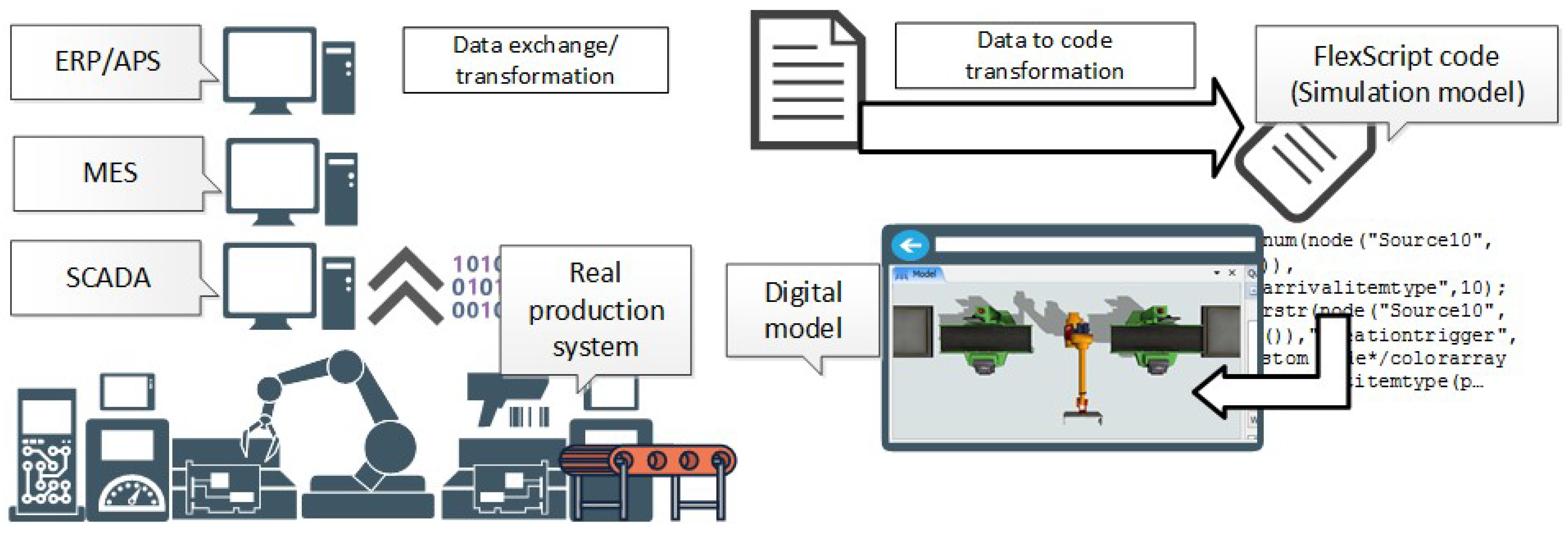
The central element of the proposed CPPS architecture is the DT based on discrete event 3D simulation models. To reflect the dynamics of the real system, the simulation model is supported by automatic generators of simulation models used in methods of semi-automatic creation and automatic updating of simulation models. Generators can be based on data mapping and transformation methods using a neutral data format and the XSL and XSLT languages [53,54]. Process data from sensors and programmable logic controllers (PLC) are transferred to the SCADA system and then to MES/ERP systems. From there, through data exchange interfaces and integration modules, the data required in the process of creating and updating the simulation model can be mapped and, depending on the needs, transformed into a neutral data model, and, then, using internal simulation software languages, transformed into code that creates a new or modifies an existing simulation model, as shown in Figure 4. This solution allows for easy practical implementation of the method because it can be used with any management system and any computer simulation system (e.g., Enterprise Dynamics, Arena, FlexSim).

Figure 4.
Digital model—indirect data exchange/transformation.
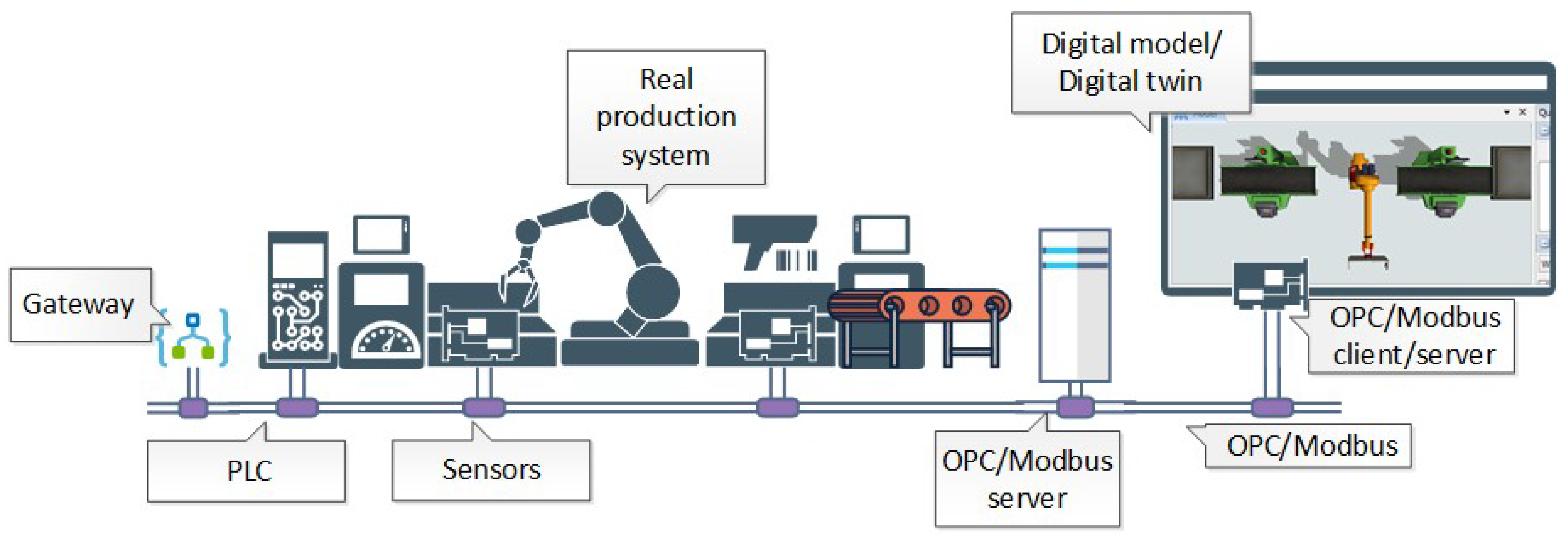
Of course, as mentioned in Section 1, the transition from a digital model to a digital twin requires that the digital model has mechanisms for a bi-directional data flow between existing physical and virtual/digital objects. For this purpose, a model–control system architecture is proposed using the so-called emulation of industrial automation system components tools directly in the simulation software. It allows to create direct connections between digital, virtual objects of the simulation system and external physical sensors, PLC controllers, or communication clients/servers. The architecture of such a solution is shown in Figure 5. The combination of solutions shown in Figure 1 and Figure 2 allows the model to be updated with data from production management systems as well as directly from sensors or PLC controllers (e.g., using OPC or Modbus protocols). This functionality is provided by, e.g., the emulation tool of the FlexSim simulation system [55]. It also makes it possible to send responses back from the DT to the planning or control system.
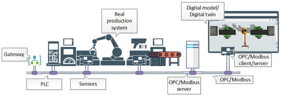
Figure 5.
greenDigital twin—direct data exchange.
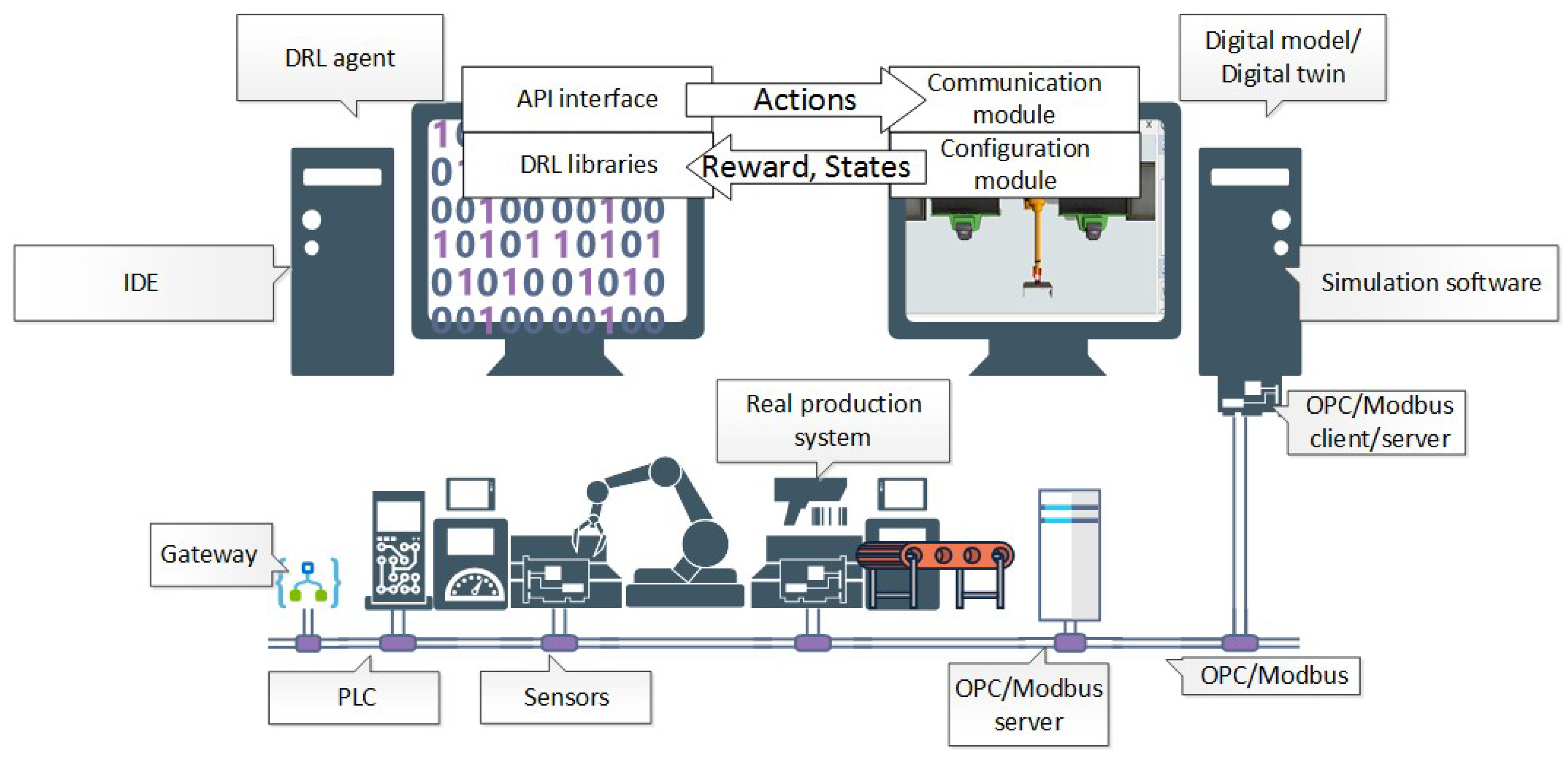
The next stage includes supplementing the cyber layer with modules enabling the use of selected RL algorithms and enabling a two-way connection between the DRL agent and the simulation model. The simulation model serves as the environment for interaction, learning, and verification of the agent’s policy. Most of the algorithms mentioned in Section 2 are publicly available in open-source libraries containing their implementations. These include popular Python libraries: OpenAI Baselines, Stable Baselines3, or keras-rl. Additionally, an API must be provided for communication between DRL agents and the environment. In the case discussed, the environment with which the agent communicates is a simulation model, so the simulation software will constitute a non-standard environment for which the design of appropriate communication and configuration modules will be required. Such modules should not only implement two-way communication, but also provide access to model configuration functions that allow, among other things, the definition of the observation space, the space of actions taken by the agent, and the reward function along with its standardization to the values required by individual algorithms. Appropriate tool packages that provide the functionality described above can be implemented directly in commercially available simulation programming using API mechanisms. The architecture of such a solution is shown in Figure 6.
Figure 6.
Cyber–Physical Production System architecture.
A practical example of the implementation of this concept is shown in the next section.
4. Experiments and Result
This section presents a practical implementation of the concept of using a DT as an interaction environment for DRL agents during training in the reinforcement learning model. First, we will briefly summarize the analyzed problem of allocating processes to resources in the production system. Then, we will describe the DT environment and the DRL model, along with state–action spaces and functions for rewarding agents for assigning tasks to production resources, respectively.
4.1. Problem Description
The problem under consideration concerns a fragment of the production system consisting of three parallel mixed-model production lines, which are sub-assembly lines for semiproducts. Semiproducts are taken from dedicated buffers to the first production cell of each line (labeled M1, M2, and M3) (Figure 7). Each buffer (Q1, Q2, and Q3) is an overhead conveyor loop with capacity . Semi-finished products flow into the system according to the arrival rate , characterized by two statistical distributions A and D, where A describes the distribution of durations between each arrival to the system, and D describes the distribution of n-versions of semi-finished products, from the following P set:
where P is the set of possible versions that can be processed in the system, and is the i-th version of semi-finished products.
Figure 7.
Production system.
The DRL agent decides on the order in which semi-finished products are routed from the buffer to the production cell. If a product is introduced into the buffer that would exceed its capacity, the product from the buffer with the longest waiting time is redirected to the adjacent buffer through a bypass connecting buffers in the system. Thus, this problem under consideration is a special case of the dynamic mixed-model sequencing problem.
Since the lead times in a production cell depend on the previous version of the product produced there, selecting a product from the buffers affects the work sequence and allows for load balancing and maximizing efficiency. Depending on the versions of the pair, the product may require additional time for processing. Therefore, the product is called a work-intensive model or version. Processing times are known and defined in the time matrix , whose columns and rows correspond to the vectors of individual product versions P:
where is the processing time of version i, if version j preceded it.
The objective is to dynamically identify a production sequence, defined by the sequence of decisions of the agent regarding the selection of products from the buffer. The quality of a production sequence is evaluated based on the total working time obtained in relation to the minimum, for a given sequence of versions:
where is the version number processed in the i-th order in the sequence, and k is the sequence length for the period considered.
In summary, the learning objective of the agent is to maximize the expected return, which is the total reward over the multiple episodes, and, in the discussed case, corresponds to the efficiency of the production cell M in a 4 h work period.
4.2. DRL Environment
4.2.1. Digital Twin—Discrete-Event Simulation Model
The simulation model constituting the environment that the DRL agent will observe and interact with during training was built in the 3D FlexSim simulation software (v.23.2.3) [56]. The digital model maps all resources of a selected part of the production system, together with the internal logistics system (Figure 8).
Figure 8.
Digital 3D simulation model.
Thanks to the data exchange interfaces and emulation tools described in Section 3, the DT can be continuously updated with process data. The use of a simulation model allows the study to include, in addition to the parameters that take into account the problem described in Section 4.1, many parameters of the intralogistics system, such as the speed of conveyors, AGVs, buffer capacity, number of carriers, etc., and their easy and quick update, by using an extensive GUI or data exchange interfaces. However, in order for the digital twin created in this way to be able to participate in the agent’s DRL training, it was necessary to develop additional modules (see Figure 6), which are described in the following subsections.
4.2.2. DRL Agent and API Interface
The DRL agent was coded and executed in Python using the stable-baselines3 libraries [57] (containing a set of DRL algorithm implementations, including A2C, DDPG, DQN, HER, PPO, and SAC) and the Gym library (providing a standard API for communication between learning algorithms and different environments) in VS Code. The designed agent uses the previously selected PPO and A2C algorithms. This choice was also dictated by the fact that, for the planned implementations, action and observation spaces can be defined in a wide range of types, such as Box, Discrete, MultiDiscrete and MultiBinary. The first can contain one or more continuous parameters, and the others can be used to capture parameters as discrete variables.
4.3. State Space, Action Space, and Reward Function
In the environment of the described case, the state space of the reinforcement learning model is defined by a tuple representing a vector, as shown in (4):
where is the number of semiproducts of the i-th version waiting in the buffer (), is the currently processed version of the product, is the processed versions preceding the current one, and l is the vector length of preceding versions.
In the model, the action can be understood as the control of the order of product allocation to the production cell at the current moment, and the action space A is the number of the version selected for processing in particular, being a discrete parameter:
where is the i-th version of semiproduct.
The reward function is set as shown in (6), which indicates the reward received by the agent after executing each joint scheduling action:
It takes values <0.1> and is the enhanced result of the ratio of the minimum execution time to the actual processing time (in response to the action taken by the agent). The reinforcement in relation to (3) is intended to give a greater reward to solutions close to the maximum and a greater penalty for choosing actions that cause large time differences.
4.4. Interface DT FlexSim–DRL Agent
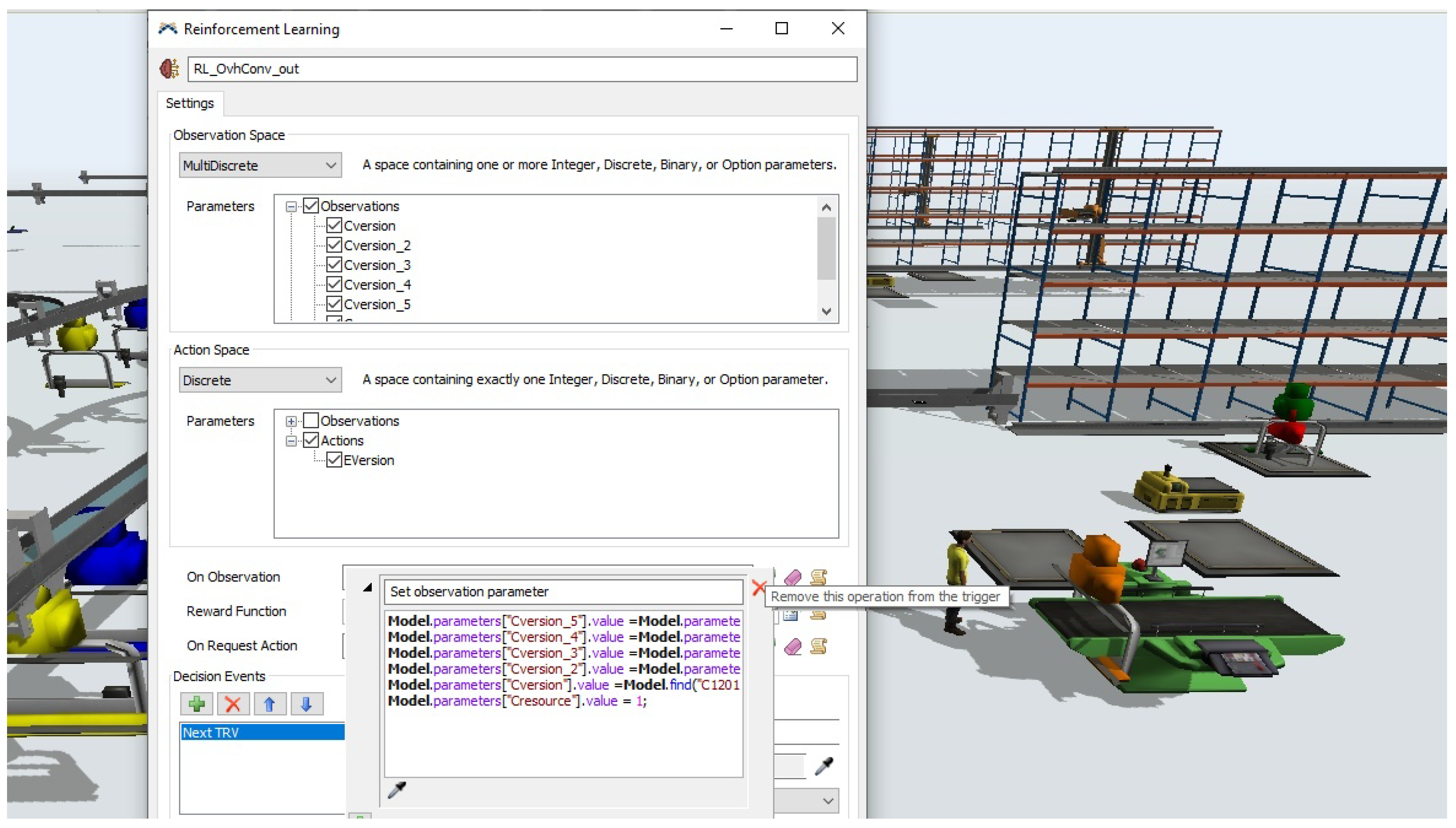
Communication between the DRL agent and the DT in the FlexSim software was accomplished using the reinforcement learning tool. This tool provides a user interface configuration that allows configuring the observation and action space and defining the reward function of decision events (Figure 9). Additionally, it provides support for connecting to the agent and handling events triggered in the agent module, such as resetting the model, starting the simulation, reading the observation space, and triggering an action. The Observation Space and Action Space containers contain controls for selecting the space type and parameters associated with the simulation model objects covering the given space. On Observation, Reward Function, and On Request action triggers are used by the reinforcement learning tool to define procedures performed during the simulation, which are, in turn, setting the parameters of the observation space just before returning them to the agent, returning the reward values and the end of the training episode marker, and passing, from the trained model, an action for the current state of the model. The last parameter—Decision Events—indicates events during the simulation when a reward will be received for the previous actions, and the observation and action will be taken.
Figure 9.
State space, action space, and reward function definition in FlexSim.
4.5. Training Process of RL Agent and Results of Experiments
The digital twin was built based on a simulation model in the FlexSim software, as described in Section 4.2, consisting of objects included in the buffer area and the M1 production cell (the first area after the inflow of semiproducts—see the gray area in Figure 7). Training experiments were conducted for such an area. The simulation model was supplemented with Interface DT FlexSim–DRL Agent modules (see Section 4.4). The training and test experiments were performed on a PC with an AMD Ryzen 5 3600 Six-Core Processor @ 3.60 GHz, and Windows 10 64-bit operating system. The simulation software, the DRL agent, and the required interfaces were installed on this platform. In the first stage, the DRL agent was trained using a DT through continuous trial and error. At each step, the agent received the reward value from the DT and assigned an action. Therefore, the agent’s actions influenced the operating sequence of the M1 production cell, and the results obtained there were subject to evaluation. Seven versions of the semiproduct were selected, the process times () of which depended on the preceding version at the considered workcell. The processing times ranged from 90 to 210 [s]. The distributions of the arrival rate and versions in the input stream to the buffer are given in the description of each experiment. The initial parameter settings for training PPO and A2C are listed in Table 1. The values of the initial DRL parameters of the algorithms were the default values introduced in the used libraries [57], set by the authors. The models were trained multiple times to achieve convergence in the training process and the highest possible reward values. Several parameters were changed, such as the total number of samples to train on, the number of steps to run for each environment per update, and the discount factor gamma. The results presented in the following subsections include only selected significant values from a series of experiments conducted on the models. In the next stage, the trained models controlled the operation of the DT in experiments to verify their effectiveness. At this stage, the same hardware platform was used to run subsequent replications of the simulation. The value of the reward function (6), corresponding to the efficiency of the production cell, was used as an the evaluation metric.

Table 1.
PPO and A2C initial parameter settings.
4.5.1. Experiment #1
In this experiment, the distribution of semiproduct versions was assumed as a uniform distribution. The arrival rate distribution was assumed to be exponential with a scale parameter of 30 [s].
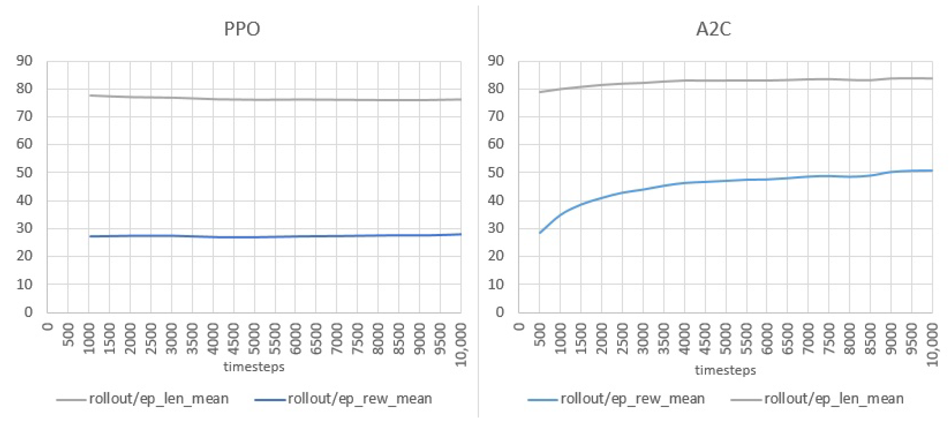
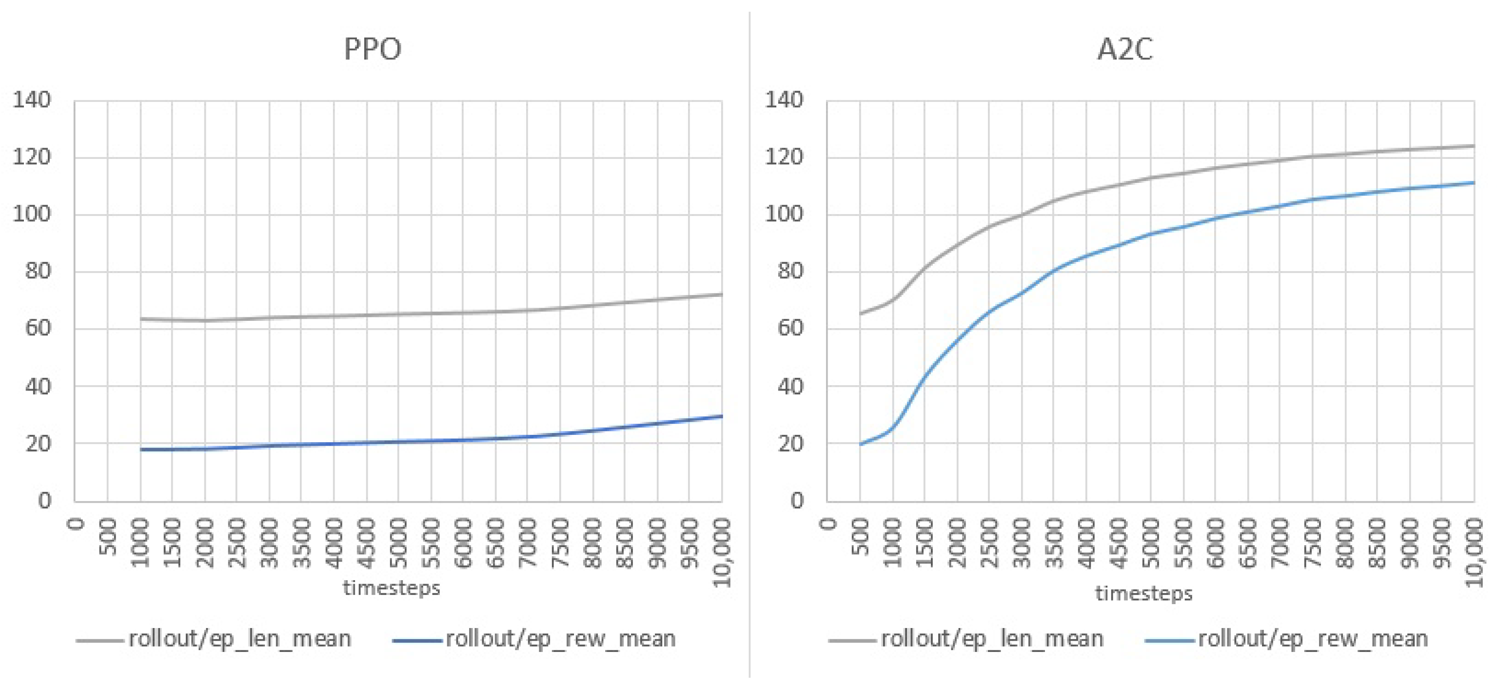
Figure 10 shows the results obtained in the training process for the PPO and A2C algorithms. The graphs show the values of the average length of the episode (ep_len_mean) and the average reward per episode (ep_rew_mean). The PPO algorithm, for default parameter values, does not obtain better results during the training process. There is a visible increase in the reward obtained for the A2C algorithm (from 30 to 50). As the agent’s observation of the environment and actions are taken after the end of processing for individual semi-finished products, the value for the length of the episode corresponds to the achieved system throughput for the assumed simulation time.
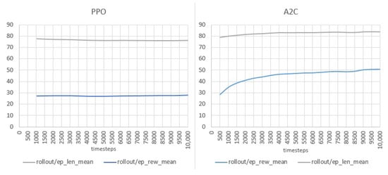
Figure 10.
Training process results for the initial parameter values of the PPO and A2C algorithms.
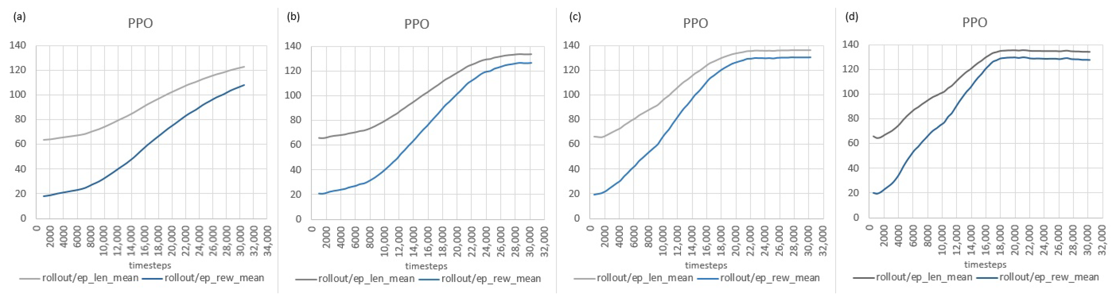
In the next step, several training sessions were performed for different values of selected parameters of the PPO algorithm (which showed no improvement for the default parameters). The changes included the total number of samples to train on, the number of steps to run for each environment per update and the discount factor gamma.
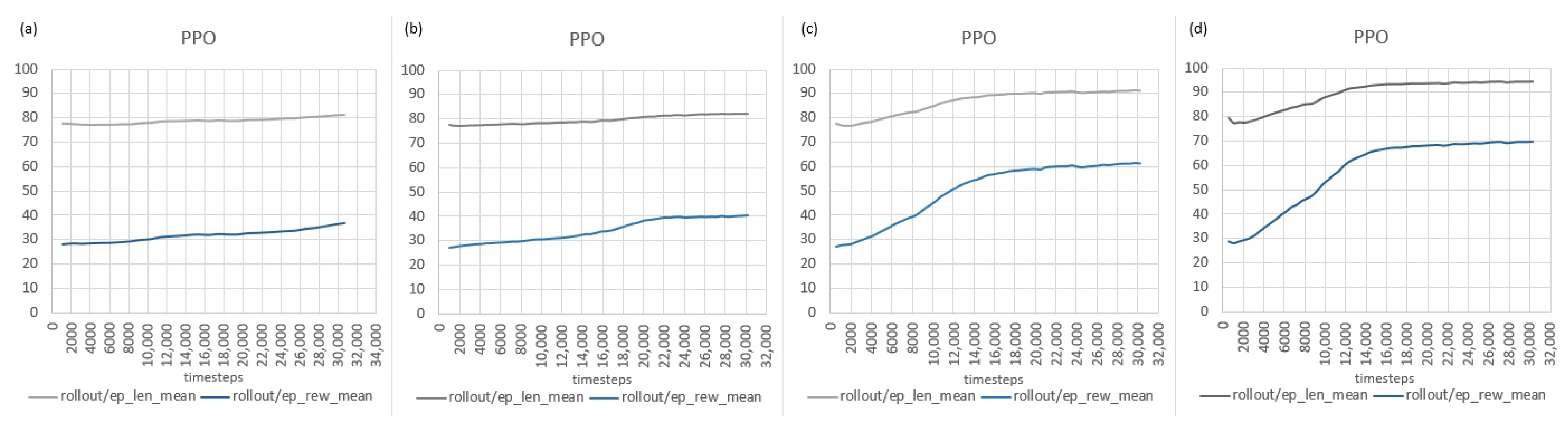
In Figure 11, the results obtained in the training process for the PPO are presented. The description shows only the values of the parameters that differ from the initial values. A significant improvement in the learning process can be seen.
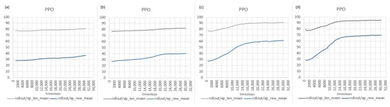
Figure 11.
Training process results for various parameter values of the PPO algorithm: (a) total_timesteps = 30,000; (b) total_timesteps = 30,000, n_steps = 512; (c) total_timesteps = 30,000, n_steps = 512, gamma = 0.89; (d) total_timesteps = 30,000, n_steps = 512, gamma = 0.69.
Table 2 synthetically shows the reward values obtained for selected parameters.
Table 2.
PPO algorithm training results.
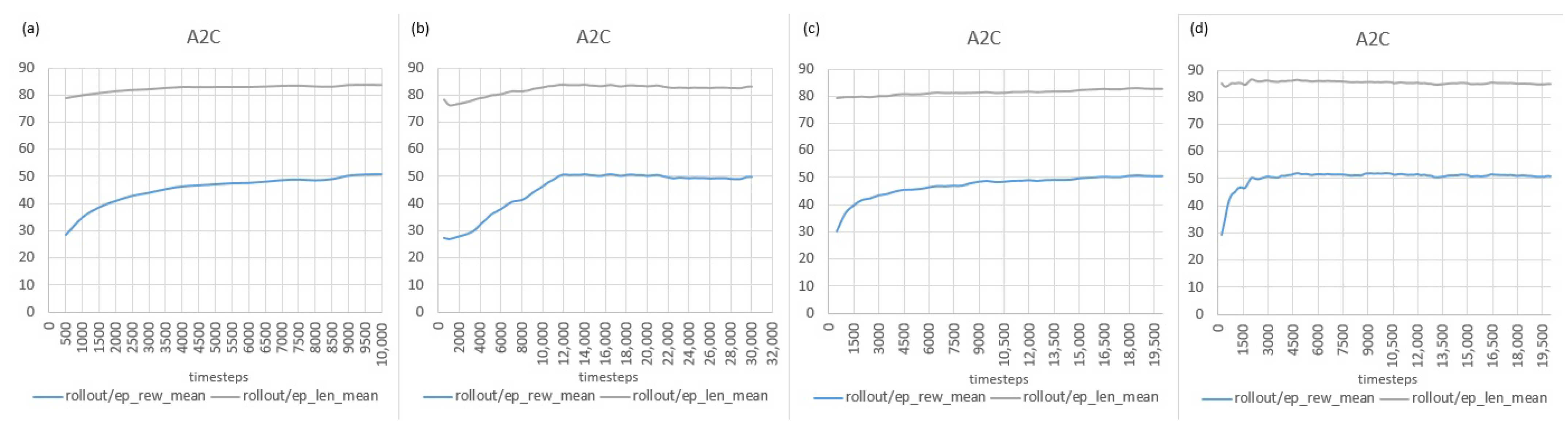
As in the case of the PPO algorithm, the next step was devoted to training the A2C algorithm for different parameter values. As before, the changes included the total number of samples to train on, the number of steps per update, and the discount factor.
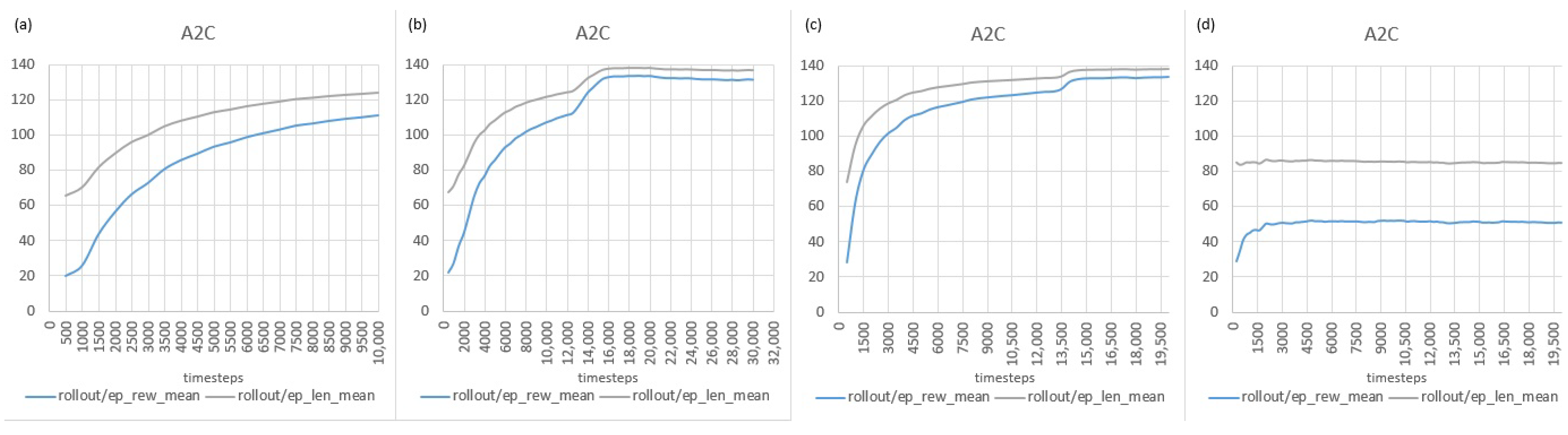
In Figure 12, the results obtained in the training process for A2C are presented. No significant improvement in learning is observed.
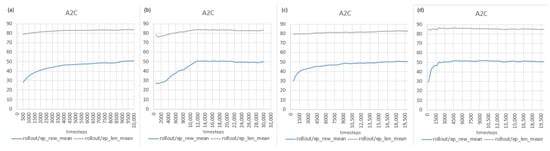
Figure 12.
Training process results for various parameter values of the A2C algorithm: (a) initial parameters; (b) total_timesteps = 30,000, n_steps = 5; (c) total_timesteps = 20,000, n_steps = 5, gamma = 0.89; (d) total_timesteps = 20,000, n_steps = 2, gamma = 0.89.
Table 3 synthetically presents the reward values obtained for selected parameters.
Table 3.
A2C algorithm training results.
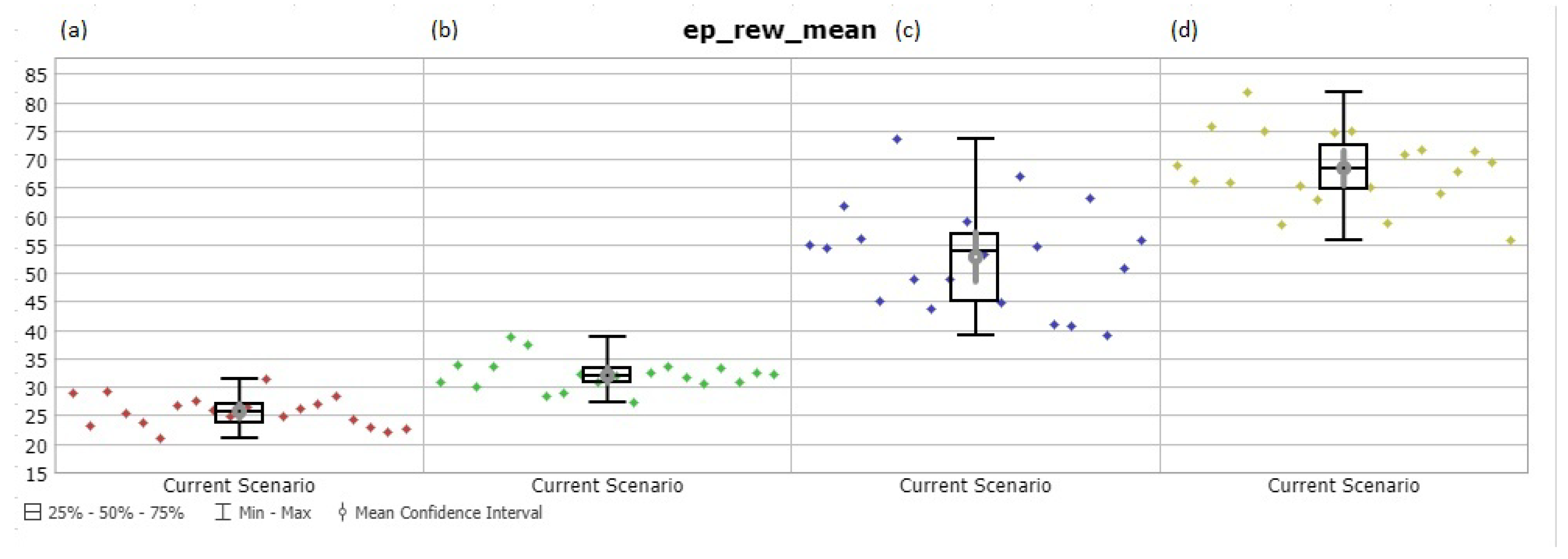
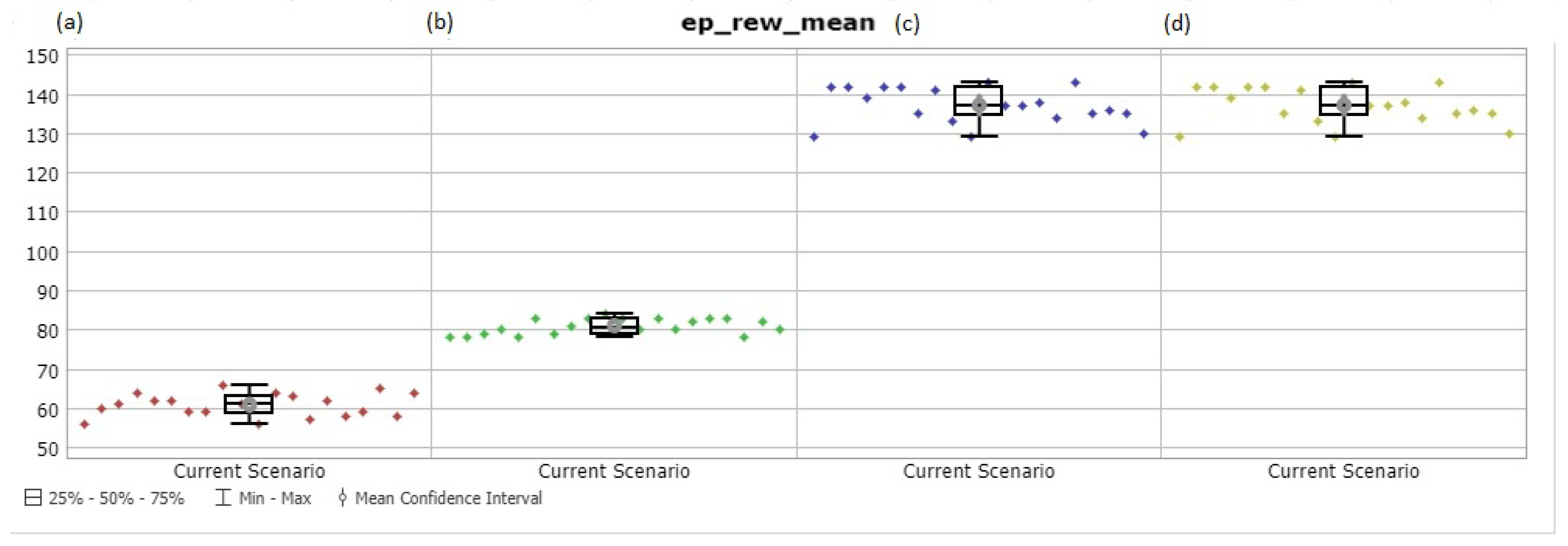
Then, the best-trained PPO and A2C models were used to control the sequence of semiproducts in the simulation environment. Figure 13a–d show the average results of the total reward for 20 replications obtained in FlexSim for the random allocation of semiproducts to the production cell, the FCFS/longest waiting time dispatching rule, the trained A2C model, and the trained PPO model.
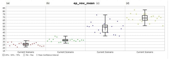
Figure 13.
Results obtained in the simulation model for trained models and dispatching rules: (a) random allocation of semiproducts; (b) FCFS/longest waiting time dispatching rule; (c) A2C-trained model, total_timesteps = 20,000, n_steps = 2, gamma = 0.89; (d) PPO-trained model, total_timesteps = 30,000, n_steps = 512, gamma = 0.69.
4.5.2. Experiment #2
In the next experiment, the distribution of versions of semiproducts entering the system was modified to reflect problems in the supply chain or changes in demand. A discretized beta distribution was assumed with parameters A = 1 and B = 3 and lower- and upper-bounds of 1 and 7.
Figure 14 shows the results obtained in the training process for the PPO and A2C algorithms for the initial data (Table 1). The charts show the values of the average length of the episode (ep_len_mean) and the average reward per episode (ep_rew_mean). The PPO algorithm, for default parameter values, achieves only a slight increase in effectiveness in the training process. However, there is a significant increase in the reward obtained for the A2C algorithm (from 20 to 110).
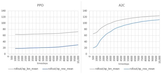
Figure 14.
Training process results for the initial parameter values of the PPO and A2C algorithms.
Then, similar to experiment #1, several training sessions were conducted for various values of selected parameters of the PPO algorithm (which was much less effective than A2C for the initial parameter values). The changes included the total number of samples to train on, the number of steps to run for each environment per update and the discount factor gamma.
In Figure 15, the results obtained in the training process for the PPO are presented. The description shows only the values of the parameters that differ from the initial values. A significant improvement in the learning process can be seen.
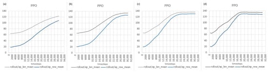
Figure 15.
Training process results for various parameter values of the PPO algorithm: (a) total_timesteps = 30,000; (b) total_timesteps = 30,000, n_steps = 512; (c) total_timesteps = 30,000, n_steps = 512, gamma = 0.89; (d) total_timesteps = 30,000, n_steps = 512, gamma = 0.69.
Table 4 synthetically shows the reward values obtained for selected parameters.
Table 4.
PPO algorithm training results.
As with the PPO algorithm, the next step was devoted to training the A2C algorithm for different parameter values. As before, the changes included the total number of samples to train on, the number of steps per update, and the discount factor.
In Figure 16, the results obtained in the training process for the A2C are presented. For cases (b) and (c), the convergence of the graphs is observed with a slight increase. Reducing the number of steps to run for each environment per update in case (d) results in the loss of the ability to improve the result in the training process.
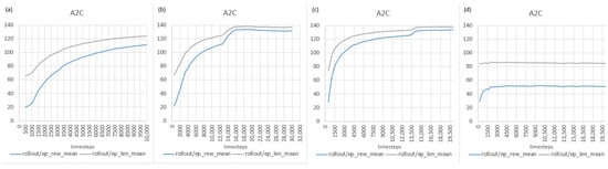
Figure 16.
Training process results for various parameter values of the A2C algorithm: (a) initial parameters; (b) total_timesteps = 30,000, n_steps = 5; (c) total_timesteps = 20,000, n_steps = 5, gamma = 0.89; (d) total_timesteps = 20,000, n_steps = 2, gamma = 0.89.
Table 5 synthetically presents the reward values obtained for selected parameters.
Table 5.
A2C algorithm training results.
Furthermore, in this experiment, the best-trained PPO and A2C models were used to control the sequence of semiproducts in the simulation environment. Figure 17a–d show the average results of the total reward for 20 replications obtained in FlexSim for the random allocation of semiproducts to the production cell, the FCFS/longest waiting time dispatching rule, the trained PPO model, and the trained A2C model.
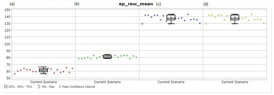
Figure 17.
Results obtained in the simulation model for trained models and dispatching rules: (a) random allocation of semiproducts; (b) FCFS/longest waiting time dispatching rule; (c) PPO-trained model total_timesteps = 30,000, n_steps = 512, gamma = 0.89; (d) A2C-trained model total_timesteps = 30,000, n_steps = 5, gamma = 0.99.
5. Discussion
Comparing the selected DRL algorithms, it can be concluded that PPO turned out to be the best for both the uniform and modified product version distributions. In the first case, it achieved a significant advantage over A2C, while, in the second case, both algorithms achieved similar, very good results of the trained model. More importantly, the results obtained in the training process were confirmed in the process of using the trained models in simulations conducted on the DT for many replications of the simulation model. As can be seen in Figure 13 and Figure 17, the obtained values of the reward function (correlated with the objective function for the problem under consideration) were at the same level as in the final phase of the training process. They also showed a significant advantage over the results for random control decisions and those based on typical dispatching rules.
The obtained results also indicate the need to perform a phase of tuning algorithm parameters for the current states of the production system mapped in the digital twin. This is most clearly visible in the results for PPO shown in Figure 11. Obtaining the convergence of the graph for case (b) could indicate achieving the maximum result in the training process. Still, the results of subsequent experiments (c) and (d) showed the possibility of improving the training results by 50%. However, as the example of the results obtained for the set of training parameters of the A2C algorithm in the case shown in Figure 16d shows, achieving convergence on the graph of the reward value versus the number of steps does not guarantee obtaining an effective trained model. In such a case, probably due to significant differences in the number of product versions arriving in the system, the too-small number of steps to run for each environment per update did not allow the agent’s policy to be adjusted to the circumstances. Moreover, general conclusions cannot be drawn here with regard to the minimum value of n_steps because, in Experiment #1, an identical set of parameter values gave the best result for the A2C algorithm for the case analyzed there. However, it is noticeable that reference values that are too low will make the agent converge prematurely, thus failing to learn the optimal decision path. Similarly, the analysis of the results in terms of the influence of variability and the discount factor gamma, where lower values place more emphasis on immediate rewards, indicates the possibility of achieving faster convergence of the training process. It can be seen in Figure 12b,c and Figure 15b,c. In the analyzed cases, however, it did not always result in a significant reduction in the learning time or the maximum reward value obtained (Figure 16b,c).
It shows that, due to the variable, dynamic nature of production systems and the wide variety of organizational and technological solutions used by manufacturers, it is recommended to always analyze the impact of the variability of parameter values on the quality of the training process. In general, there is a noticeable possibility of significantly shortening the training process through a preliminary analysis of the impact of parameters on the speed of the training process. In particular, it can be seen in the results obtained for A2C (Figure 16b,c) and PPO (Figure 11c,d), where, already, in the middle of the training process, the trend of the reward gradually converges to the highest value, indicating that the model training is completed.
Furthermore, RL agent training and verifying the learned model in the simulation-based DT and RL agent combination architecture proposed in this paper allows for a simple and fast reconfiguration of the environment with which the agent interacts. Compared to architectures based on non-simulation environments, a brief overview of which is presented in Section 1, changing the components or performance indicators of the system on which the reward function is based, which, in the case of analytical models, would involve the need to construct new formulas or mathematical models, does not constitute any problem and it is quick and simple. This is due to the fact that, in the proposed approach, the values of the reward function can be directly linked to the statistics of the components of the simulation model and the modification of the reward function comes down to indicating them in the communication modules (see Figure 9). In addition, using simple predefined conditional blocks, it is possible to create dynamic functions that activate various statistics depending on the adopted conditions. Similarly, changing the structure of the simulation model in response to changes in the real production system can be done automatically or semi-automatically by connecting the model to enterprise information systems or automation devices.
The limitations of the presented architecture are mainly related to the scope of the digital representation of real objects. Most modern advanced simulation software contains extensive libraries of predefined objects, covering manufacturing, assembly, and logistics subsystems. However, due to the wide variety of technologies and production organization in different industries, some model objects still have to be created from scratch. Similarly, current simulation systems have not transferred all the communication protocols used in industrial automation to the digital layer.
The key challenge remains to transfer the discussed solutions as quickly as possible into industrial practice. Partial challenges, including providing a framework for data transfer and real-time communication capabilities, and developing common data models and guidelines for implementation are related to it. The challenges in the closely related aspects of cybersecurity and explainable AI should also be mentioned. Furthermore, there is an important future need to ensure compliance of the designed industrial solutions with the legal requirements to which solutions used in industrial practice based on AI methods will be subject, especially in the context of the ongoing work on the AI Act [58].
6. Conclusions
The paper presents the Cyber–Physical Production System architecture based on a digital twin, in which the digital virtual equivalent of the production system is a simulation model. The DT becomes the environment with which the reinforcement learning agent interacts. As shown in the experimental part, the proposed architecture can be practically implemented using advanced 3D simulation software and open-source available libraries. It allows for fast and easy implementation in an industrial operating environment. The implementation of industrial research in this area is of great importance in verifying the possibility of using AI methods, including DRL methods, in operational problems. Due to the significant diversity and dynamics in the planning and control processes of today’s complex production systems, it is difficult to develop and verify solutions only in an offline environment. The DT solution presented in this paper, connected to and mapping the states of a real system or process, can simultaneously train DRL agents and verify the obtained answers for the current conditions. Such verified results obtained for the trained model can then be implemented in operational conditions with much lower risk. The DT, being connected to the objects of the real system, will also be able to verify the effectiveness of the currently used trained model preventively. If changes are detected in the conditions of the production system or its environment, it will be able to run the training process for new conditions in parallel, in the background, and transfer it to the control system quickly.
Further research will concern industrial research related to testing digital twins’ communication and interaction methods based on the proposed architecture at the level of industrial demonstrators.
Funding
Publication supported as part of the Excellence Initiative—Research University program implemented at the Silesian University of Technology, year 2024 (grant number 10/020/SDU/10-21-02).
Institutional Review Board Statement
Not applicable.
Informed Consent Statement
Not applicable.
Data Availability Statement
The original contributions presented in the study are included in the article, further inquiries can be directed to the corresponding author.
Conflicts of Interest
The authors declare no conflicts of interest.
Abbreviations
The following abbreviations are used in this manuscript:
| A3C | Asynchronous Advantage Actor–Critic |
| CPS | Cyber–physical system |
| CPPS | Cyber–Physical Production System |
| DQN | Deep Q- Network |
| DDPG | Deep Deterministic Policy Gradients |
| DRL | Deep reinforcement learning |
| DT | Digital twin |
| DTMS | Digital Twin-based Manufacturing System |
| PPO | Proximal Policy Optimization |
| RL | Reinforcement learning |
| SAC | Soft Actor–Critic |
| SARSA | State–Action–Reward–State–Action |
References
- Juhlin, P.; Schlake, J.C.; Janka, D.; Hawlitschek, A. Metamodeling of Cyber-Physical Production Systems using AutomationML for Collaborative Innovation. In Proceedings of the 2021 26th IEEE International Conference on Emerging Technologies and Factory Automation (ETFA), Vasteras, Sweden, 7–10 September 2021; pp. 1–4. [Google Scholar] [CrossRef]
- Temelkova, M. Similarities and Differences Between the Technological Paradigms “Production System”, “Cyber-physical System” and “Cyber-physical Production System”. In Proceedings of the 2022 International Conference on Communications, Information, Electronic and Energy Systems (CIEES), Veliko Tarnovo, Bulgaria, 24–26 November 2022; pp. 1–7. [Google Scholar] [CrossRef]
- Thoben, K.D.; Wiesner, S.; Wuest, T. “Industrie 4.0” and Smart Manufacturing—A Review of Research Issues and Application Examples. Int. J. Autom. Technol. 2017, 11, 4–16. [Google Scholar] [CrossRef]
- Ryalat, M.; ElMoaqet, H.; AlFaouri, M. Design of a Smart Factory Based on Cyber-Physical Systems and Internet of Things towards Industry 4.0. Appl. Sci. 2023, 13, 2156. [Google Scholar] [CrossRef]
- Martinez-Ruedas, C.; Flores-Arias, J.M.; Moreno-Garcia, I.M.; Linan-Reyes, M.; Bellido-Outeiriño, F.J. A Cyber—Physical System Based on Digital Twin and 3D SCADA for Real-Time Monitoring of Olive Oil Mills. Technologies 2024, 12, 60. [Google Scholar] [CrossRef]
- Coching, J.K.; Pe, A.J.L.; Yeung, S.G.D.; Akeboshi, W.W.N.; Billones, R.K.C. Cyber-Physical System Modeling for Bottleneck Analysis of the Manufacturing Production Line of Core Machines. In Proceedings of the 2022 IEEE International Smart Cities Conference (ISC2), Pafos, Cyprus, 26–29 September 2022; pp. 1–7. [Google Scholar] [CrossRef]
- Son, Y.H.; Park, K.T.; Lee, D.; Jeon, S.W.; Do Noh, S. Digital twin—Based cyber-physical system for automotive body production lines. Int. J. Adv. Manuf. Technol. 2021, 115, 291–310. [Google Scholar] [CrossRef]
- Monostori, L.; Kádár, B.; Bauernhansl, T.; Kondoh, S.; Kumara, S.; Reinhart, G.; Sauer, O.; Schuh, G.; Sihn, W.; Ueda, K. Cyber-physical systems in manufacturing. CIRP Ann. 2016, 65, 621–641. [Google Scholar] [CrossRef]
- Müller, T.; Jazdi, N.; Schmidt, J.P.; Weyrich, M. Cyber-physical production systems: Enhancement with a self-organized reconfiguration management. Procedia CIRP 2021, 99, 549–554. [Google Scholar] [CrossRef]
- Chakroun, A.; Hani, Y.; Elmhamedi, A.; Masmoudi, F. Digital Transformation Process of a Mechanical Parts Production workshop to fulfil the Requirements of Industry 4.0. In Proceedings of the 2022 14th International Colloquium of Logistics and Supply Chain Management (LOGISTIQUA), El Jadida, Morocco, 25–27 May 2022; pp. 1–6. [Google Scholar] [CrossRef]
- Flores-García, E.; Kim, G.Y.; Yang, J.; Wiktorsson, M.; Do Noh, S. Analyzing the Characteristics of Digital Twin and Discrete Event Simulation in Cyber Physical Systems. In Proceedings of the Advances in Production Management Systems. Towards Smart and Digital Manufacturing; Lalic, B., Majstorovic, V., Marjanovic, U., von Cieminski, G., Romero, D., Eds.; Springer International Publishing: Cham, Switzerland, 2020; pp. 238–244. [Google Scholar]
- Ricondo, I.; Porto, A.; Ugarte, M. A digital twin framework for the simulation and optimization of production systems. Procedia CIRP 2021, 104, 762–767. [Google Scholar] [CrossRef]
- Coito, T.; Faria, P.; Martins, M.S.E.; Firme, B.; Vieira, S.M.; Figueiredo, J.; Sousa, J.M.C. Digital Twin of a Flexible Manufacturing System for Solutions Preparation. Automation 2022, 3, 153–175. [Google Scholar] [CrossRef]
- Monek, G.D.; Fischer, S. IIoT-Supported Manufacturing-Material-Flow Tracking in a DES-Based Digital-Twin Environment. Infrastructures 2023, 8, 75. [Google Scholar] [CrossRef]
- Rosen, R.; von Wichert, G.; Lo, G.; Bettenhausen, K.D. About The Importance of Autonomy and Digital Twins for the Future of Manufacturing. IFAC-PapersOnLine 2015, 48, 567–572. [Google Scholar] [CrossRef]
- Kritzinger, W.; Karner, M.; Traar, G.; Henjes, J.; Sihn, W. Digital Twin in manufacturing: A categorical literature review and classification. IFAC-PapersOnLine 2018, 51, 1016–1022. [Google Scholar] [CrossRef]
- Zhuang, C.; Liu, J.; Xiong, H. Digital twin-based smart production management and control framework for the complex product assembly shop-floor. Int. J. Adv. Manuf. Technol. 2018, 96, 1149–1163. [Google Scholar] [CrossRef]
- Liu, S.; Zheng, P.; Jinsong, B. Digital Twin-based manufacturing system: A survey based on a novel reference model. J. Intell. Manuf. 2023, 1–30. [Google Scholar] [CrossRef]
- Panzer, M.; Bender, B. Deep reinforcement learning in production systems: A systematic literature review. Int. J. Prod. Res. 2022, 60, 4316–4341. [Google Scholar] [CrossRef]
- Wang, X.; Zhang, L.; Liu, Y.; Laili, Y. An improved deep reinforcement learning-based scheduling approach for dynamic task scheduling in cloud manufacturing. Int. J. Prod. Res. 2024, 62, 4014–4030. [Google Scholar] [CrossRef]
- Guzman, E.; Andres, B.; Poler, R. Models and algorithms for production planning, scheduling and sequencing problems: A holistic framework and a systematic review. J. Ind. Inf. Integr. 2022, 27, 100287. [Google Scholar] [CrossRef]
- Lei, Y.; Deng, Q.; Liao, M.; Gao, S. Deep reinforcement learning for dynamic distributed job shop scheduling problem with transfers. Expert Syst. Appl. 2024, 251, 123970. [Google Scholar] [CrossRef]
- Yang, S.; Xu, Z.; Wang, J. Intelligent Decision-Making of Scheduling for Dynamic Permutation Flowshop via Deep Reinforcement Learning. Sensors 2021, 21, 1019. [Google Scholar] [CrossRef]
- Huang, J. Mixed-batch scheduling to minimize total tardiness using deep reinforcement learning. Appl. Soft Comput. 2024, 160, 111699. [Google Scholar] [CrossRef]
- Li, C.; Zheng, P.; Yin, Y.; Wang, B.; Wang, L. Deep reinforcement learning in smart manufacturing: A review and prospects. CIRP J. Manuf. Sci. Technol. 2023, 40, 75–101. [Google Scholar] [CrossRef]
- Cunha, B.; Madureira, A.M.; Fonseca, B.; Coelho, D. Deep Reinforcement Learning as a Job Shop Scheduling Solver: A Literature Review. In Proceedings of the Hybrid Intelligent Systems; Madureira, A.M., Abraham, A., Gandhi, N., Varela, M.L., Eds.; Springer International Publishing: Cham, Switzerland, 2020; pp. 350–359. [Google Scholar] [CrossRef]
- Luo, S. Dynamic scheduling for flexible job shop with new job insertions by deep reinforcement learning. Appl. Soft Comput. 2020, 91, 106208. [Google Scholar] [CrossRef]
- Liu, C.L.; Chang, C.C.; Tseng, C.J. Actor-Critic Deep Reinforcement Learning for Solving Job Shop Scheduling Problems. IEEE Access 2020, 8, 71752–71762. [Google Scholar] [CrossRef]
- Park, I.B.; Park, J. Scalable Scheduling of Semiconductor Packaging Facilities Using Deep Reinforcement Learning. IEEE Trans. Cybern. 2023, 53, 3518–3531. [Google Scholar] [CrossRef]
- Onggo, B.S. Symbiotic Simulation System (S3) for Industry 4.0. In Simulation for Industry 4.0: Past, Present, and Future; Gunal, M.M., Ed.; Springer International Publishing: Cham, Switzerland, 2019; pp. 153–165. [Google Scholar] [CrossRef]
- Ma, Y.; Cai, J.; Li, S.; Liu, J.; Xing, J.; Qiao, F. Double deep Q-network-based self-adaptive scheduling approach for smart shop floor. Neural Comput. Appl. 2023, 35, 1–16. [Google Scholar] [CrossRef]
- Sutton, R.S.; Barto, A.G. Reinforcement Learning: An Introduction, 2nd ed.; MIT Press: Cambridge, MA, USA, 2018. [Google Scholar]
- 10 Breakthrough Technologies 2017. MIT Technology Review. 2017. Available online: https://www.technologyreview.com/magazines/10-breakthrough-technologies-2017/ (accessed on 30 April 2024).
- Tang, Z.; Xu, X.; Shi, Y. Grasp Planning Based on Deep Reinforcement Learning: A Brief Survey. In Proceedings of the 2021 China Automation Congress (CAC), Beijing, China, 22–24 October 2021; pp. 7293–7299. [Google Scholar] [CrossRef]
- Arulkumaran, K.; Deisenroth, M.P.; Brundage, M.; Bharath, A.A. Deep Reinforcement Learning: A Brief Survey. IEEE Signal Process. Mag. 2017, 34, 26–38. [Google Scholar] [CrossRef]
- Dong, H.; Ding, Z.; Zhang, S. Deep Reinforcement Learning Fundamentals, Research and Applications: Fundamentals, Research and Applications; Springer: Singapore, 2020. [Google Scholar] [CrossRef]
- Silver, D.; Hubert, T.; Schrittwieser, J.; Antonoglou, I.; Lai, M.; Guez, A.; Lanctot, M.; Sifre, L.; Kumaran, D.; Graepel, T.; et al. Mastering Chess and Shogi by Self-Play with a General Reinforcement Learning Algorithm. arXiv 2017, arXiv:1712.01815. [Google Scholar]
- Wang, X.; Wang, S.; Liang, X.; Zhao, D.; Huang, J.; Xu, X.; Dai, B.; Miao, Q. Deep Reinforcement Learning: A Survey. IEEE Trans. Neural Netw. Learn. Syst. 2024, 35, 5064–5078. [Google Scholar] [CrossRef]
- Shyalika, C.; Silva, T.P.; Karunananda, A.S. Reinforcement Learning in Dynamic Task Scheduling: A Review. SN Comput. Sci. 2020, 1, 306. [Google Scholar] [CrossRef]
- Watkins, C.J.C.H.; Dayan, P. Q-learning. Mach. Learn. 1992, 8, 279–292. [Google Scholar] [CrossRef]
- Jiang, H.; Wang, H.; Yau, W.Y.; Wan, K.W. A Brief Survey: Deep Reinforcement Learning in Mobile Robot Navigation. In Proceedings of the 2020 15th IEEE Conference on Industrial Electronics and Applications (ICIEA), Kristiansand, Norway, 9–13 November 2020; pp. 592–597. [Google Scholar] [CrossRef]
- Mnih, V.; Kavukcuoglu, K.; Silver, D.; Rusu, A.A.; Veness, J.; Bellemare, M.G.; Graves, A.; Riedmiller, M.; Fidjeland, A.K.; Ostrovski, G.; et al. Human-level control through deep reinforcement learning. Nature 2015, 518, 529–533. [Google Scholar] [CrossRef]
- Schulman, J.; Wolski, F.; Dhariwal, P.; Radford, A.; Klimov, O. Proximal Policy Optimization Algorithms. arXiv 2017, arXiv:1707.06347. [Google Scholar]
- Wu, Y.; Mansimov, E.; Liao, S.; Radford, A.; Schulman, J. OpenAI Baselines: ACKTR & A2C. 2017. Available online: https://openai.com/index/openai-baselines-acktr-a2c/ (accessed on 30 April 2024).
- Kang, Z.; Catal, C.; Tekinerdogan, B. Machine learning applications in production lines: A systematic literature review. Comput. Ind. Eng. 2020, 149, 106773. [Google Scholar] [CrossRef]
- Matulis, M.; Harvey, C. A robot arm digital twin utilising reinforcement learning. Comput. Graph. 2021, 95, 106–114. [Google Scholar] [CrossRef]
- Liu, G.; Sun, W.; Xie, W.; Xu, Y. Learning visual path–following skills for industrial robot using deep reinforcement learning. Int. J. Adv. Manuf. Technol. 2022, 122, 1099–1111. [Google Scholar] [CrossRef]
- Sierra-García, J.E.; Santos, M. Control of Industrial AGV Based on Reinforcement Learning. In Proceedings of the 15th International Conference on Soft Computing Models in Industrial and Environmental Applications (SOCO 2020), Burgos, Spain, 16–18 September 2020; Herrero, Á., Cambra, C., Urda, D., Sedano, J., Quintián, H., Corchado, E., Eds.; Springer International Publishing: Cham, Switzerland, 2021; pp. 647–656. [Google Scholar]
- Pan, G.; Xiang, Y.; Wang, X.; Yu, Z.; Zhou, X. Research on path planning algorithm of mobile robot based on reinforcement learning. Soft Comput. 2022, 26, 8961–8970. [Google Scholar] [CrossRef]
- Lee, J.H.; Kim, H.J. Reinforcement learning for robotic flow shop scheduling with processing time variations. Int. J. Prod. Res. 2022, 60, 2346–2368. [Google Scholar] [CrossRef]
- Zhang, J.; Guo, B.; Ding, X.; Hu, D.; Tang, J.; Du, K.; Tang, C.; Jiang, Y. An adaptive multi-objective multi-task scheduling method by hierarchical deep reinforcement learning. Appl. Soft Comput. 2024, 154, 111342. [Google Scholar] [CrossRef]
- Han, B.A.; Yang, J.J. Research on Adaptive Job Shop Scheduling Problems Based on Dueling Double DQN. IEEE Access 2020, 8, 186474–186495. [Google Scholar] [CrossRef]
- Krenczyk, D.; Bocewicz, G. Data-Driven Simulation Model Generation for ERP and DES Systems Integration. In Proceedings of the Intelligent Data Engineering and Automated Learning—IDEAL, Wroclaw, Poland, 14–16 October 2015; Jackowski, K., Burduk, R., Walkowiak, K., Wozniak, M., Yin, H., Eds.; Springer International Publishing: Cham, Switzerland, 2015; pp. 264–272. [Google Scholar] [CrossRef]
- Krenczyk, D. Dynamic simulation models as digital twins of logistics systems driven by data from multiple sources. J. Phys. Conf. Ser. 2022, 2198, 012059. [Google Scholar] [CrossRef]
- Flexsim, Emulation Tool—Emulation Overview. Available online: https://docs.flexsim.com/en/24.1/Reference/Tools/Emulation/EmulationOverview/EmulationOverview.html (accessed on 30 April 2024).
- Beaverstock, M.; Greenwood, A.; Nordgren, W. Applied Simulation: Modeling and Analysis Using Flexsim; BookBaby: Pennsauken, NJ, USA, 2018. [Google Scholar]
- Raffin, A.; Hill, A.; Gleave, A.; Kanervisto, A.; Ernestus, M.; Dormann, N. Stable-Baselines3: Reliable Reinforcement Learning Implementations. J. Mach. Learn. Res. 2021, 22, 1–8. [Google Scholar]
- AI Act, European Commission. 2024. Available online: https://digital-strategy.ec.europa.eu/en/policies/regulatory-framework-ai (accessed on 15 May 2024).


Disclaimer/Publisher’s Note: The statements, opinions and data contained in all publications are solely those of the individual author(s) and contributor(s) and not of MDPI and/or the editor(s). MDPI and/or the editor(s) disclaim responsibility for any injury to people or property resulting from any ideas, methods, instructions or products referred to in the content. |
© 2024 by the author. Licensee MDPI, Basel, Switzerland. This article is an open access article distributed under the terms and conditions of the Creative Commons Attribution (CC BY) license (https://creativecommons.org/licenses/by/4.0/).