
Visualization of Demodulated Sound Based on Sequential Acoustic Ray Tracing with Self-Demodulation in Parametric Array Loudspeakers


Abstract
1. Introduction
2. Principles of Parametric Array Loudspeakers
3. Proposed Self-Demodulation-Based Visualization Method
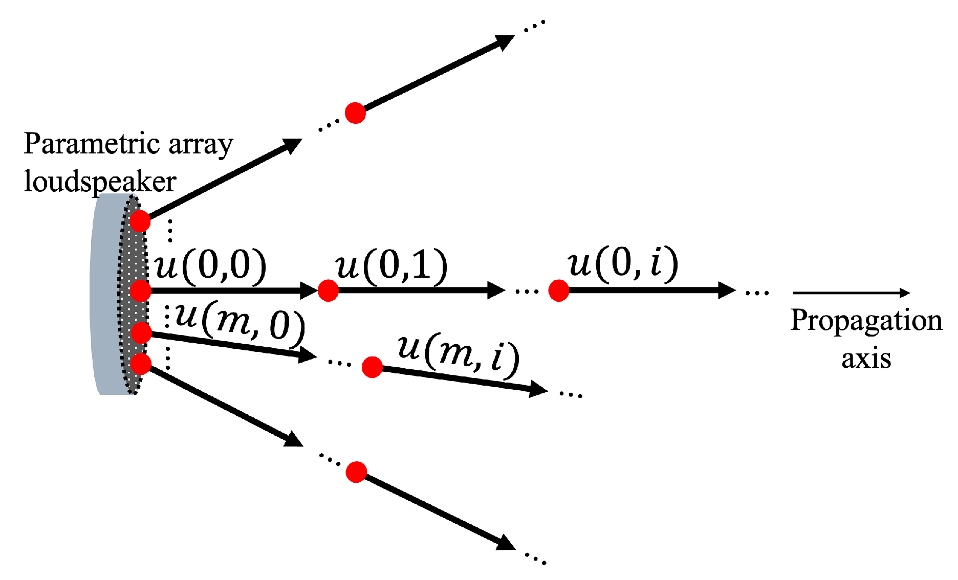
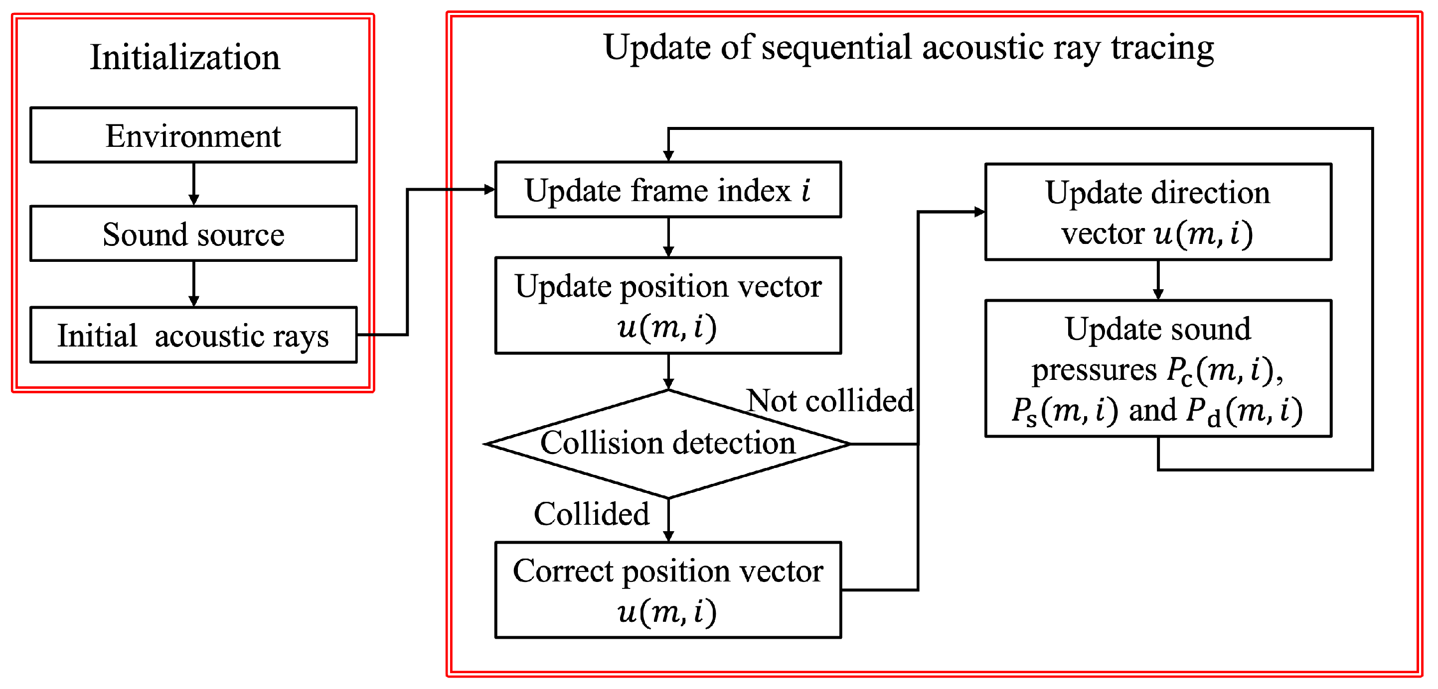
3.1. Overview of the Proposed Method
- The ray index m is defined to identify the original positions.
- A position vector is defined as the starting position for each ray.
- The direction vector is defined as the direction of each ray, where .
- The sound pressure is defined as the sound pressure of the carrier wave at frequency .
- The sound pressure is defined for each sideband wave at frequency .
- The sound pressure is defined as the demodulated sound pressure at frequency .
- The virtual source intensity is defined as the intensity of the virtual source at frequency .
3.2. Simulation Initialization
- Step 1: The initialization of the environment
- Step 2: The initialization of the sound source
- Step 3: The initialization of the initial acoustic rays
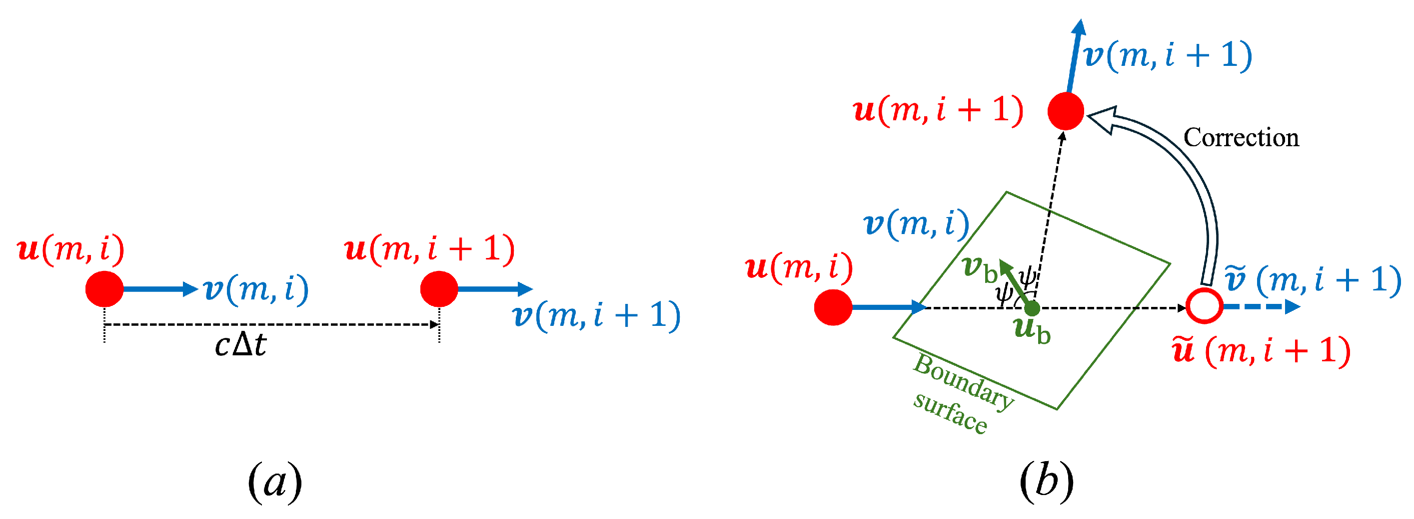
3.3. Sequential Update of Acoustic Rays
3.4. Computational Complexity of the Proposed Method
4. Evaluation Experiments
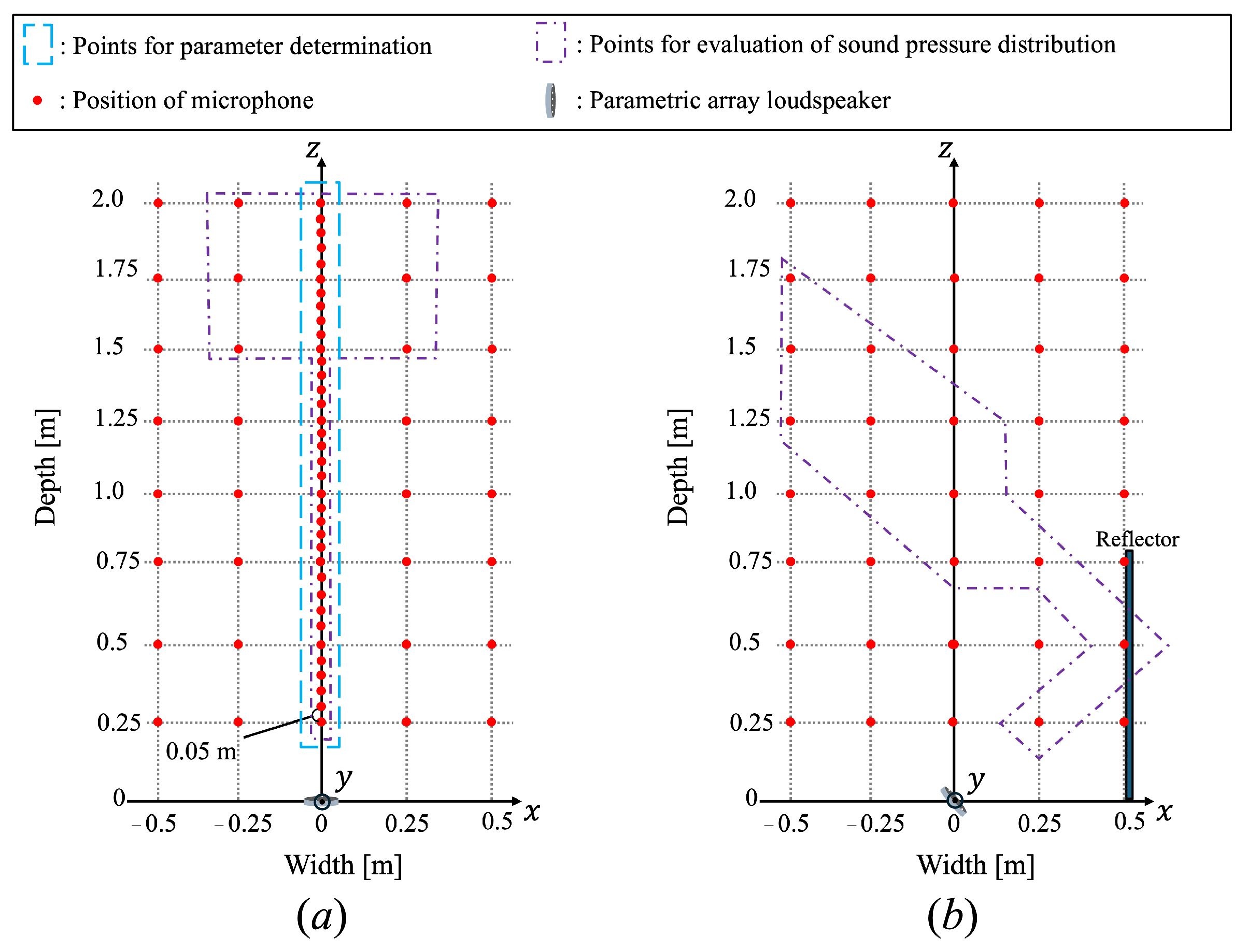
4.1. Experimental Conditions
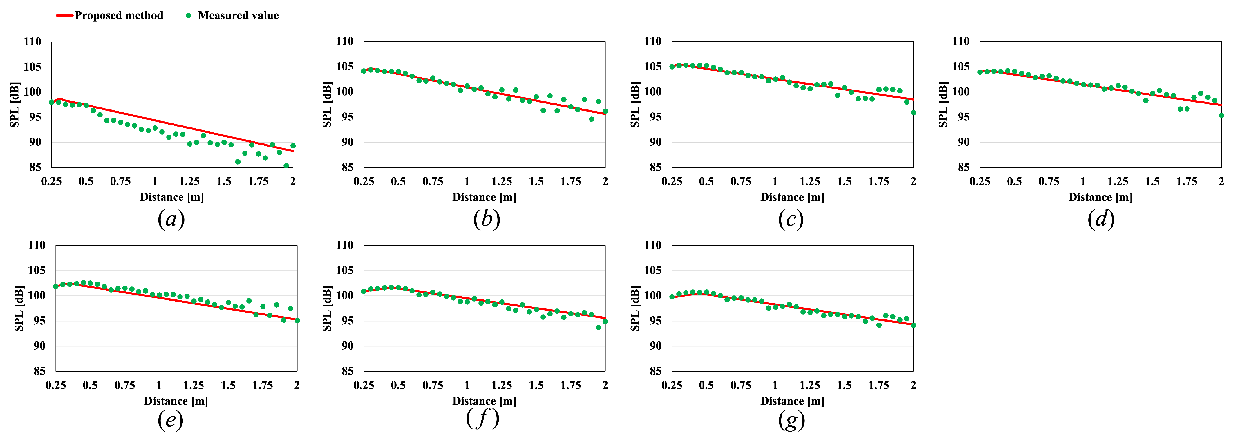
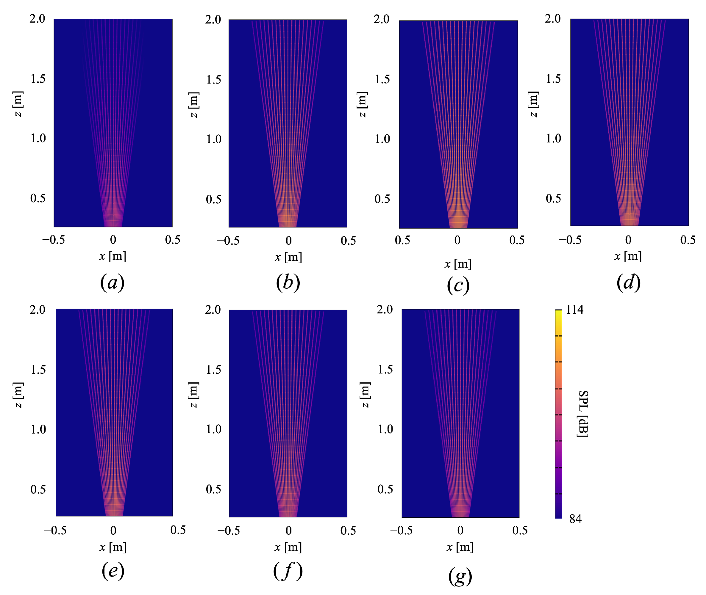
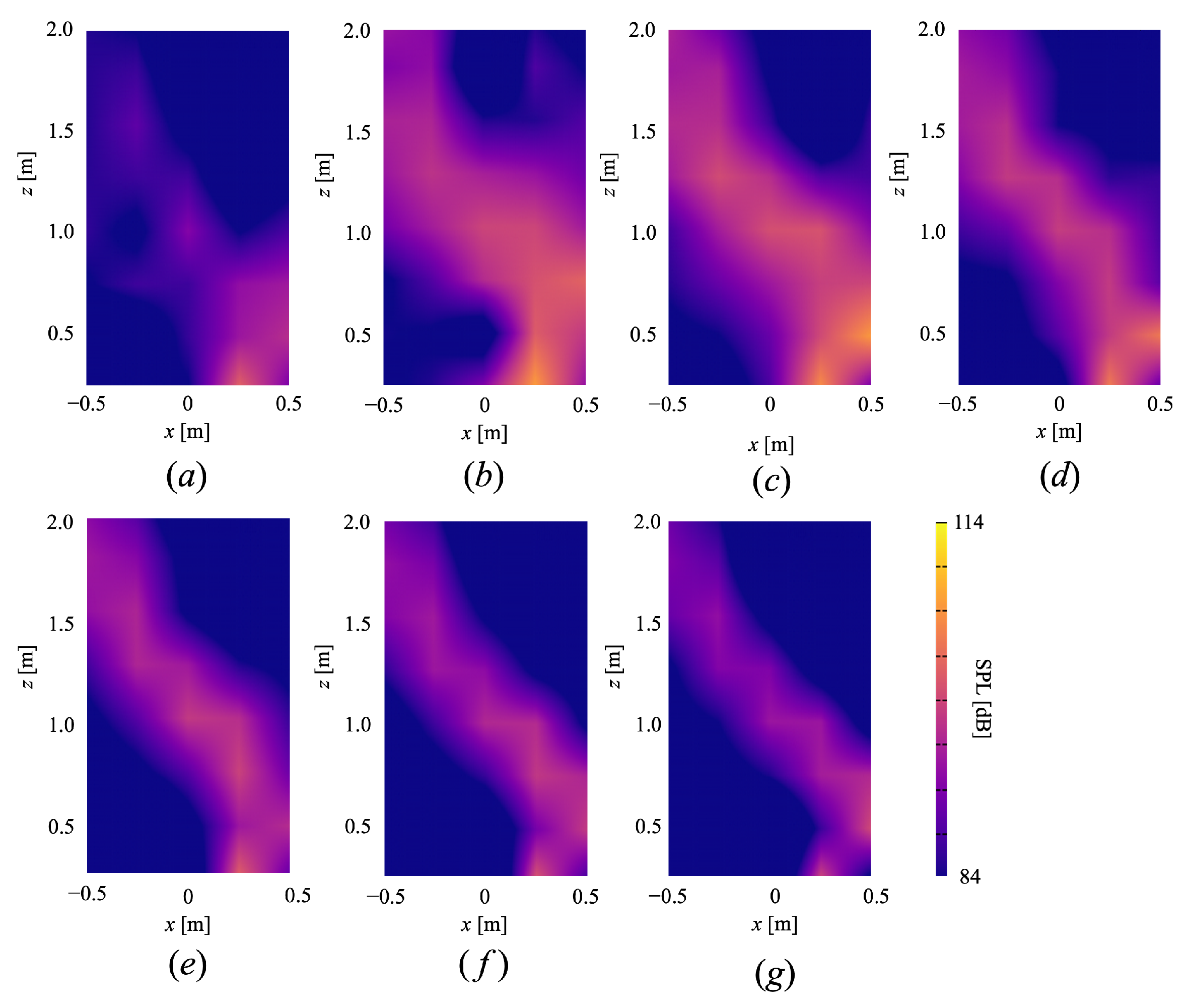
4.2. Experimental Results
5. Conclusions
Author Contributions
Funding
Data Availability Statement
Conflicts of Interest
References
- Vorländer, M. Computer simulations in room acoustics: Concepts and uncertainties. J. Acoust. Soc. Am. 2013, 133, 1203–1213. [Google Scholar] [CrossRef] [PubMed]
- Gao, H.; Feng, X.; Shen, Y. Weighted Loudspeaker Placement Method for Sound Field Reproduction. IEEE/ACM Trans. Audio Speech Lang. Process. 2022, 30, 1263–1276. [Google Scholar] [CrossRef]
- Koyama, S.; Chardon, G.; Daudet, L. Optimizing Source and Sensor Placement for Sound Field Control: An Overview. IEEE/ACM Trans. Audio, Speech, Lang. Process. 2020, 28, 696–714. [Google Scholar] [CrossRef]
- Zhu, M.; Zhao, S. An iterative approach to optimize loudspeaker placement for multi-zone sound field reproduction. J. Acoust. Soc. Am. 2021, 149, 3462–3468. [Google Scholar] [CrossRef] [PubMed]
- Bilbao, S. 3D Interpolation in Wave-Based Acoustic Simulation. IEEE Signal Process. Lett. 2022, 29, 384–388. [Google Scholar] [CrossRef]
- Bilbao, S.; Hamilton, B. Directional Sources in Wave-Based Acoustic Simulation. IEEE/ACM Trans. Audio Speech Lang. Process. 2019, 27, 415–428. [Google Scholar] [CrossRef]
- Yoshida, T.; Okuzono, T.; Sakagami, K. Binaural Auralization of Room Acoustics with a Highly Scalable Wave-Based Acoustics Simulation. Appl. Sci. 2023, 13, 2832. [Google Scholar] [CrossRef]
- Savioja, L.; Svensson, U.P. Overview of geometrical room acoustic modeling techniques. J. Acoust. Soc. Am. 2015, 138, 708–730. [Google Scholar] [CrossRef]
- Binek, W.; Pilch, A.; Kamisiński, T. Direct application of the diffusers’ reflection patterns in geometrical acoustics simulations. Appl. Acoust. 2022, 198, 108949. [Google Scholar] [CrossRef]
- Mozaffarzadeh, M.; Verweij, M.D.; de Jong, N.; Renaud, G. Comparison of Phase-Screen and Geometry-Based Phase Aberration Correction Techniques for Real-Time Transcranial Ultrasound Imaging. Appl. Sci. 2022, 12, 10183. [Google Scholar] [CrossRef]
- Reddy, J.N. An Introduction to the Finite Element Method, 3rd ed.; McGraw-Hill Education: New York, NY, USA, 2006. [Google Scholar]
- Barbieri, R.; Barbieri, N. Finite element acoustic simulation based shape optimization of a muffler. Appl. Acoust. 2006, 67, 346–357. [Google Scholar] [CrossRef]
- Marburg, S.; Nolte, B. Computational Acoustics of Noise Propagation in Fluids: Finite and Boundary Element Methods; Springer: Berlin/Heidelberg, Germany, 2008; Volume 578. [Google Scholar]
- Bai, M.R. Application of BEM (boundary element method)-based acoustic holography to radiation analysis of sound sources with arbitrarily shaped geometries. J. Acoust. Soc. Am. 1992, 92, 533–549. [Google Scholar] [CrossRef]
- Yuan, X.; Borup, D.; Wiskin, J.; Berggren, M.; Johnson, S. Simulation of acoustic wave propagation in dispersive media with relaxation losses by using FDTD method with PML absorbing boundary condition. IEEE Trans. Ultrason. Ferroelectr. Freq. Control 1999, 46, 14–23. [Google Scholar] [CrossRef] [PubMed]
- Van Mourik, J.; Murphy, D. Explicit Higher-Order FDTD Schemes for 3D Room Acoustic Simulation. IEEE/ACM Trans. Audio Speech Lang. Process. 2014, 22, 2003–2011. [Google Scholar] [CrossRef]
- Cingolani, M.; Fratoni, G.; Barbaresi, L.; D’Orazio, D.; Hamilton, B.; Garai, M. A Trial Acoustic Improvement in a Lecture Hall with MPP Sound Absorbers and FDTD Acoustic Simulations. Appl. Sci. 2021, 11, 2445. [Google Scholar] [CrossRef]
- Pind, F.; Jeong, C.H.; Hesthaven, J.S.; Engsig-Karup, A.P.; Strømann-Andersen, J. A phenomenological extended-reaction boundary model for time-domain wave-based acoustic simulations under sparse reflection conditions using a wave splitting method. Appl. Acoust. 2021, 172, 107596. [Google Scholar] [CrossRef]
- Brankovic, M.; Everett, M.E. A Method for Modeling Acoustic Waves in Moving Subdomains. Acoustics 2022, 4, 394–405. [Google Scholar] [CrossRef]
- Borish, J. Extension of the image model to arbitrary polyhedra. J. Acoust. Soc. Am. 1984, 75, 1827–1836. [Google Scholar] [CrossRef]
- Rajapaksha, T.; Qiu, X.; Cheng, E.; Burnett, I. Geometrical room geometry estimation from room impulse responses. In Proceedings of the 2016 IEEE International Conference on Acoustics, Speech and Signal Processing (ICASSP), Shanghai, China, 20–25 March 2016; pp. 331–335. [Google Scholar] [CrossRef]
- Vorländer, M. Simulation of the transient and steady-state sound propagation in rooms using a new combined ray-tracing/image-source algorithm. J. Acoust. Soc. Am. 1989, 86, 172–178. [Google Scholar] [CrossRef]
- Funkhouser, T.; Tsingos, N.; Carlbom, I.; Elko, G.; Sondhi, M.; West, J.E.; Pingali, G.; Min, P.; Ngan, A. A beam tracing method for interactive architectural acoustics. J. Acoust. Soc. Am. 2004, 115, 739–756. [Google Scholar] [CrossRef]
- Westervelt, P.J. Parametric Acoustic Array. J. Acoust. Soc. Am. 1963, 35, 535–537. [Google Scholar] [CrossRef]
- Gan, W.S.; Yang, J.; Kamakura, T. A review of parametric acoustic array in air. Appl. Acoust. 2012, 73, 1211–1219. [Google Scholar] [CrossRef]
- Sugibayashi, Y.; Kurimoto, S.; Ikefuji, D.; Morise, M.; Nishiura, T. Three-dimensional acoustic sound field reproduction based on hybrid combination of multiple parametric loudspeakers and electrodynamic subwoofer. Appl. Acoust. 2012, 73, 1282–1288. [Google Scholar] [CrossRef]
- Geng, Y.; Nakayama, M.; Nishiura, T. Narrow-edged beamforming based on individual phase inversion in amplitude-modulated wave for parametric array loudspeaker. Appl. Acoust. 2022, 200, 109060. [Google Scholar] [CrossRef]
- Geng, Y.; Nakayama, M.; Nishiura, T. Demodulated sound quality improvement for harmonic sounds in over-boosted parametric array loudspeaker. Appl. Acoust. 2022, 186, 108460. [Google Scholar] [CrossRef]
- Miyachi, T.; Balvig, J.J.; Kisada, W.; Hayakawa, K.; Suzuki, T.; Howlett, R.J.; Jain, L. A Quiet Navigation for Safe Crosswalk by Ultrasonic Beams. In Proceedings of the Knowledge-Based Intelligent Information and Engineering Systems, Vietri sul Mare, Italy, 12–14 September 2007; Springer: Berlin/Heidelberg, Germany, 2007; pp. 1049–1057. [Google Scholar]
- Tanaka, N.; Tanaka, M. Active noise control using a steerable parametric array loudspeaker. J. Acoust. Soc. Am. 2010, 127, 3526–3537. [Google Scholar] [CrossRef] [PubMed]
- Sayama, S.; Ogami, Y.; Nakayama, M.; Nishiura, T. Acoustic Space-Sharing with Multiple Parametric Array Loudspeakers for Daily Sports and Exercise. In Proceedings of the Forum Acusticum, Lyon, France, 7–11 December 2020; pp. 2599–2605. [Google Scholar] [CrossRef]
- Geng, Y.; Sayama, S.; Nakayama, M.; Nishiura, T. Movable virtual sound source construction based on wave field synthesis using a linear parametric loudspeaker array. APSIPA Trans. Signal Inf. Process. 2023, 12, e14. [Google Scholar] [CrossRef]
- Geng, Y.; Nakayama, M.; Nishiura, T. Narrow-edged Acoustical Beamforming Utilizing Phase Inversion for Frequency Modulation-based Parametric Array Loudspeaker. In Proceedings of the 2023 Asia Pacific Signal and Information Processing Association Annual Summit and Conference (APSIPA ASC), Taipei, Taiwan, 31 October–3 November 2023; pp. 2287–2293. [Google Scholar] [CrossRef]
- Thuras, A.L.; Jenkins, R.T.; O’Neil, H.T. Extraneous Frequencies Generated in Air Carrying Intense Sound Waves. J. Acoust. Soc. Am. 1935, 6, 173–180. [Google Scholar] [CrossRef]
- Nomura, H.; Hedberg, C.M.; Kamakura, T. Numerical simulation of parametric sound generation and its application to length-limited sound beam. Appl. Acoust. 2012, 73, 1231–1238. [Google Scholar] [CrossRef]
- Shimokata, M.; Nakayama, M.; Nishiura, T. Visualization of demodulated sound based on sequential acoustic-ray-tracing for parametric array loudspeakers in three-dimensional space. In Proceedings of the INTER-NOISE and NOISE-CON Congress and Conference Proceedings. Institute of Noise Control Engineering, Seoul, Republic of Korea, 23–36 August 2020; Volume 261, pp. 3839–3850. [Google Scholar]
- Kimura, K.; Yamamoto, K. A method for measuring oblique incidence absorption coefficient of absorptive panels by stretched pulse technique. Appl. Acoust. 2001, 62, 617–632. [Google Scholar] [CrossRef]


| Environment | Soundproof room (Width: 2.3 m/Depth: 3.2 m/Height: 2.2 m) |
| Ambient noise level | dB |
| Reverberation time | ms |
| Frame interval | ms |
| Carrier frequency | kHz |
| Sideband frequency | kHz |
| Demodulated frequency | kHz |
| Applied voltage | 15 V |
| Ultrasonic sound pressure meter | RION, UN-14 |
| Microphone | Sennheiser, MKH 8020 |
| A/D, D/A converter | RME, Fireface UFX |
| Power amplifier | JVC, PS-A2002 |
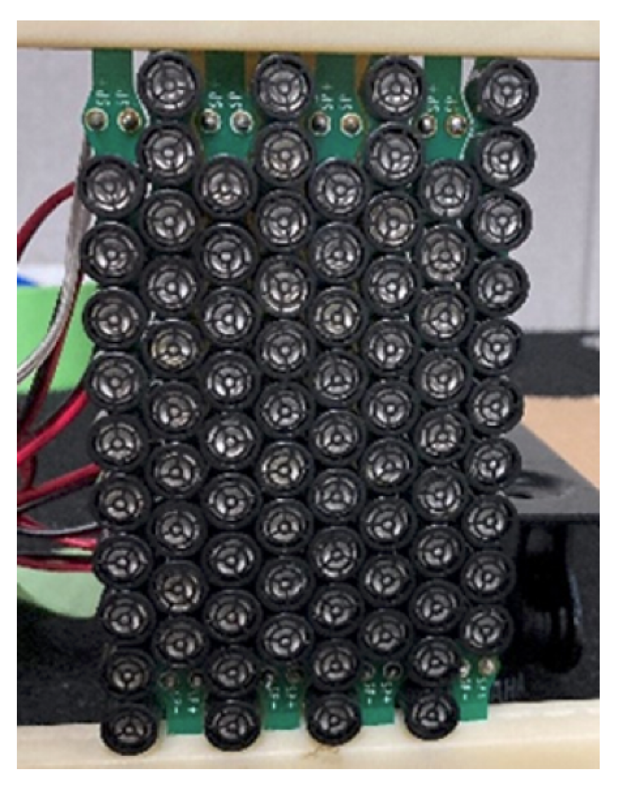
| Ultrasonic transducer | SPL Limited, UT1007-Z325R |
| Demodulated frequency (kHz) | 1 | 2 | 3 | 4 | 5 | 6 | 7 |
| Sideband frequency (kHz) | 39 | 38 | 37 | 36 | 35 | 34 | 33 |
| Ratio of sound pressure | 1.0 (reference) | 0.76 | 0.28 | 8.2 | 2.8 | 1.5 | 8.8 |
| Evaluation Area | Demodulated Frequency (kHz) | ||||||
|---|---|---|---|---|---|---|---|
| 1 | 2 | 3 | 4 | 5 | 6 | 7 | |
| Points for parameter determination | 1.94 | 0.87 | 0.83 | 0.81 | 0.93 | 0.65 | 0.52 |
| Points for evaluation (without reflection) | 2.15 | 1.14 | 1.39 | 1.13 | 1.16 | 0.98 | 1.26 |
| Points for evaluation (with reflection) | 2.48 | 1.89 | 2.28 | 2.94 | 4.23 | 4.25 | 4.95 |
| Evaluation Area | Demodulated Frequency (kHz) | ||||||
|---|---|---|---|---|---|---|---|
| 1 | 2 | 3 | 4 | 5 | 6 | 7 | |
| Points for parameter determination | 1.67 | 0.64 | 0.62 | 0.59 | 0.73 | 0.46 | 0.42 |
| Points for evaluation (without reflection) | 1.84 | 0.81 | 0.90 | 0.75 | 0.90 | 0.63 | 0.71 |
| Points for evaluation (with reflection) | 1.93 | 1.26 | 1.90 | 2.22 | 3.13 | 3.22 | 3.67 |
Disclaimer/Publisher’s Note: The statements, opinions and data contained in all publications are solely those of the individual author(s) and contributor(s) and not of MDPI and/or the editor(s). MDPI and/or the editor(s) disclaim responsibility for any injury to people or property resulting from any ideas, methods, instructions or products referred to in the content. |
© 2024 by the authors. Licensee MDPI, Basel, Switzerland. This article is an open access article distributed under the terms and conditions of the Creative Commons Attribution (CC BY) license (https://creativecommons.org/licenses/by/4.0/).
Share and Cite
Geng, Y.; Shimokata, M.; Nakayama, M.; Nishiura, T. Visualization of Demodulated Sound Based on Sequential Acoustic Ray Tracing with Self-Demodulation in Parametric Array Loudspeakers. Appl. Sci. 2024, 14, 5241. https://doi.org/10.3390/app14125241
Geng Y, Shimokata M, Nakayama M, Nishiura T. Visualization of Demodulated Sound Based on Sequential Acoustic Ray Tracing with Self-Demodulation in Parametric Array Loudspeakers. Applied Sciences. 2024; 14(12):5241. https://doi.org/10.3390/app14125241
Chicago/Turabian StyleGeng, Yuting, Makoto Shimokata, Masato Nakayama, and Takanobu Nishiura. 2024. "Visualization of Demodulated Sound Based on Sequential Acoustic Ray Tracing with Self-Demodulation in Parametric Array Loudspeakers" Applied Sciences 14, no. 12: 5241. https://doi.org/10.3390/app14125241
APA StyleGeng, Y., Shimokata, M., Nakayama, M., & Nishiura, T. (2024). Visualization of Demodulated Sound Based on Sequential Acoustic Ray Tracing with Self-Demodulation in Parametric Array Loudspeakers. Applied Sciences, 14(12), 5241. https://doi.org/10.3390/app14125241