


Parameter Calibration of Discrete Element Model of Wine Lees Particles


Abstract
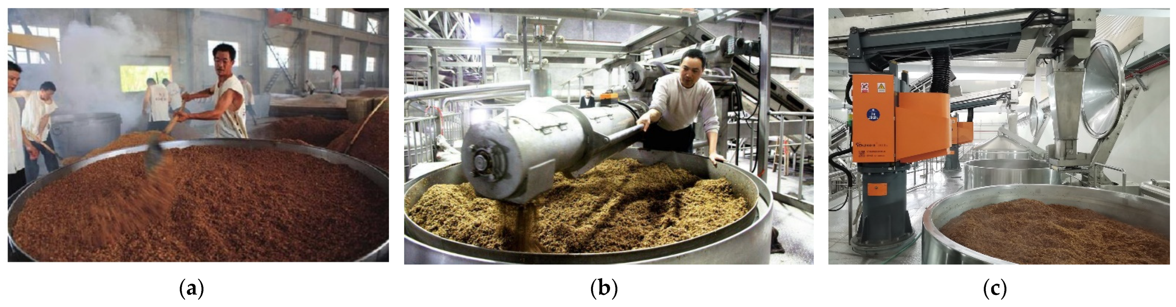
1. Introduction
2. Materials and Methods
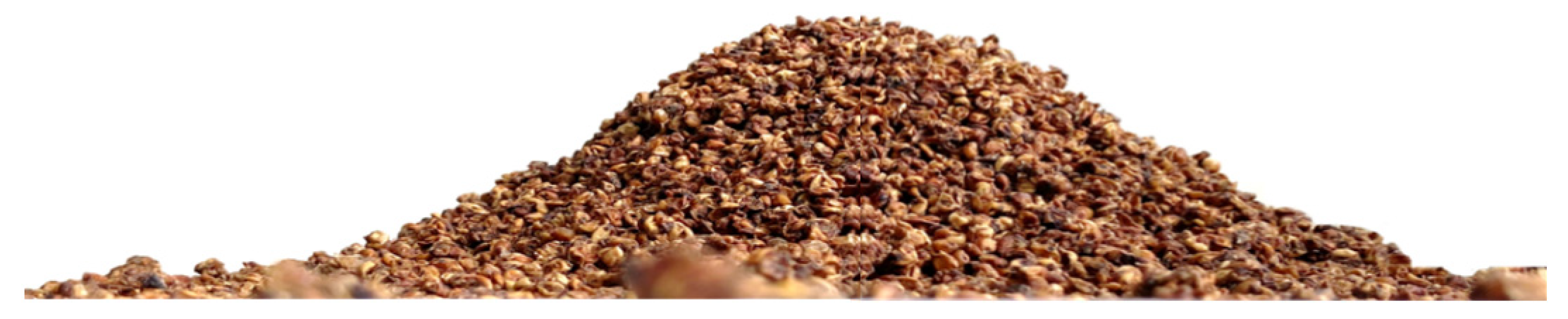
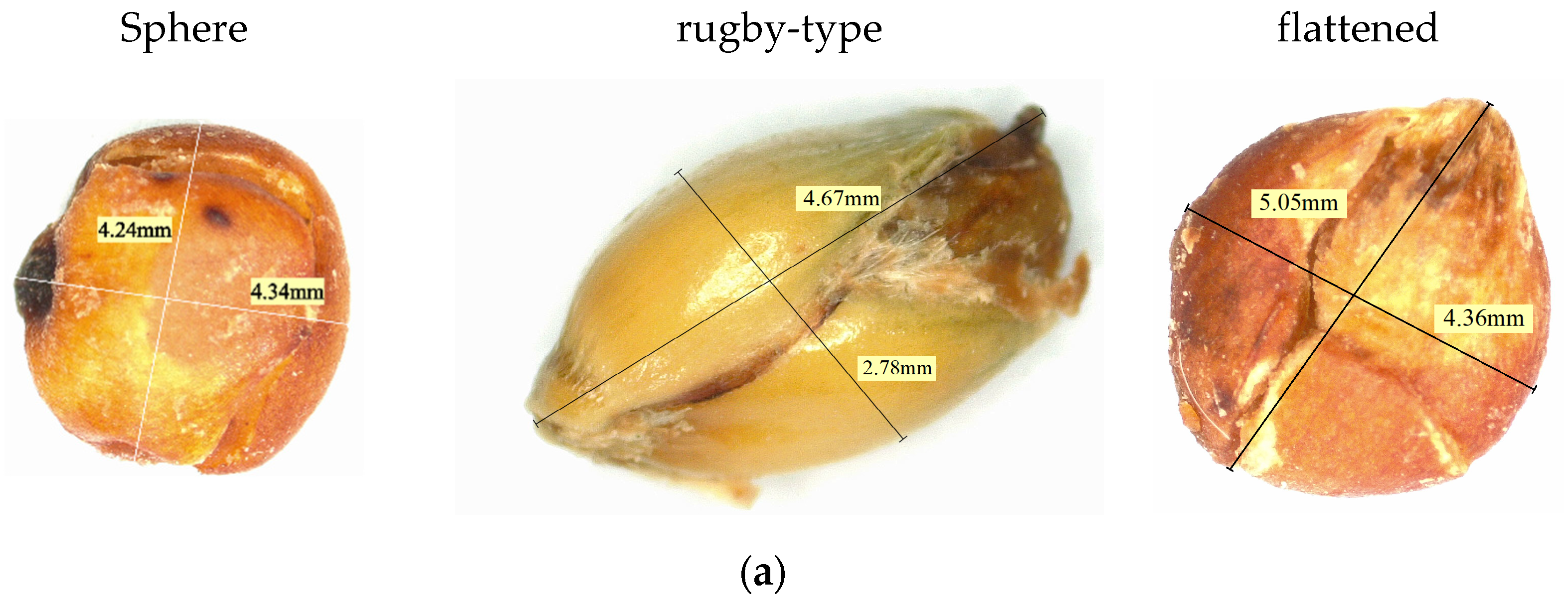
2.1. Basic Parameters of Lees Particles
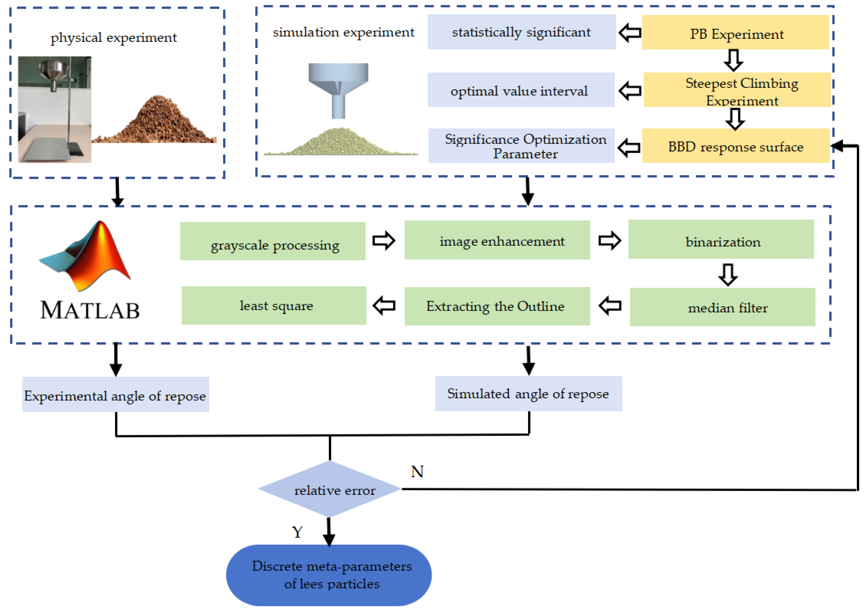
2.2. Experimental Methods
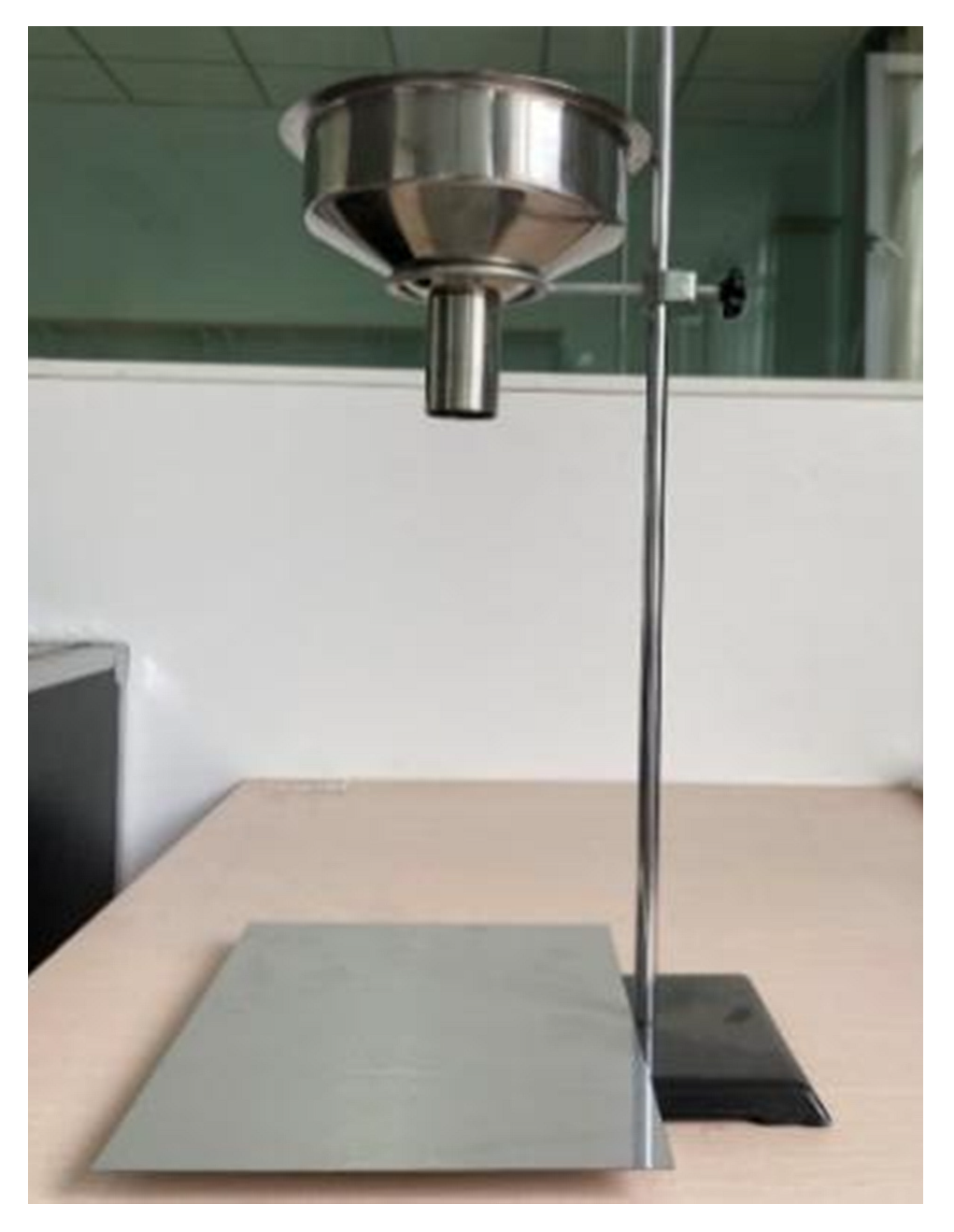
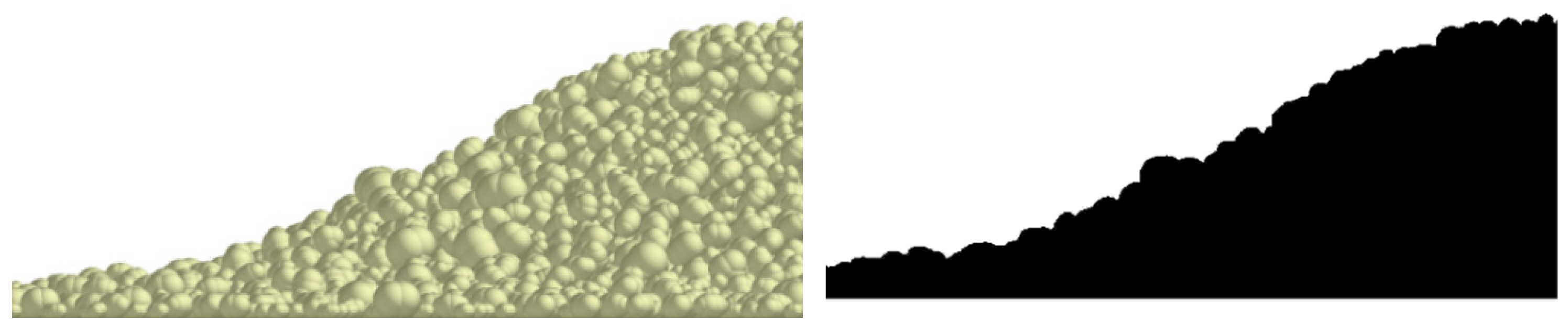
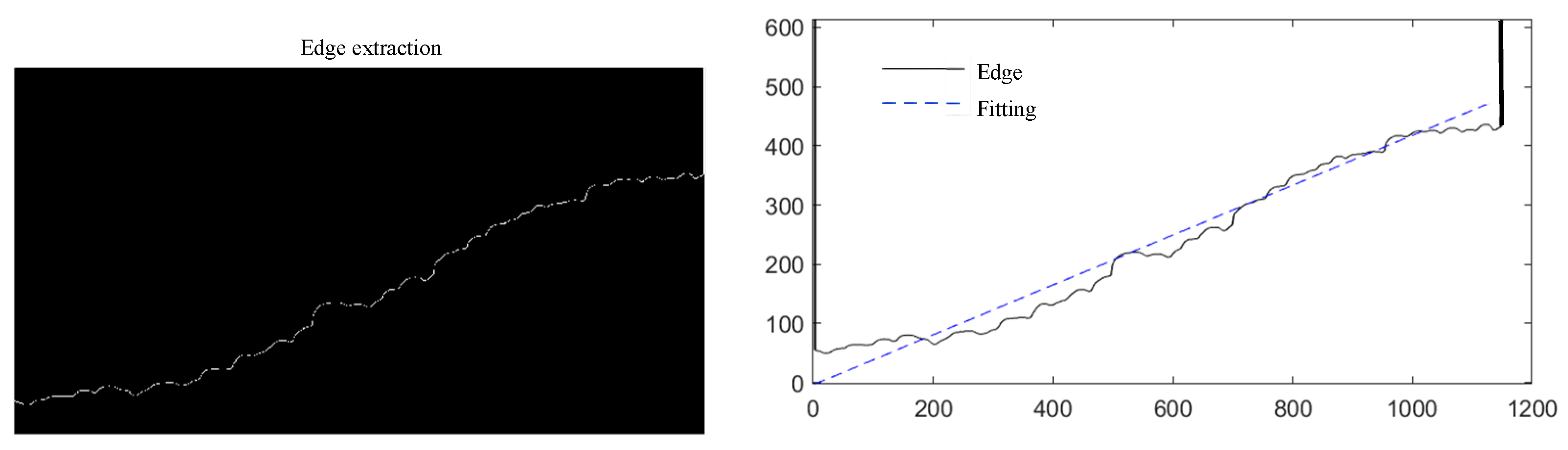
2.3. Angle of Repose Physical Tests
2.4. Simulation Models
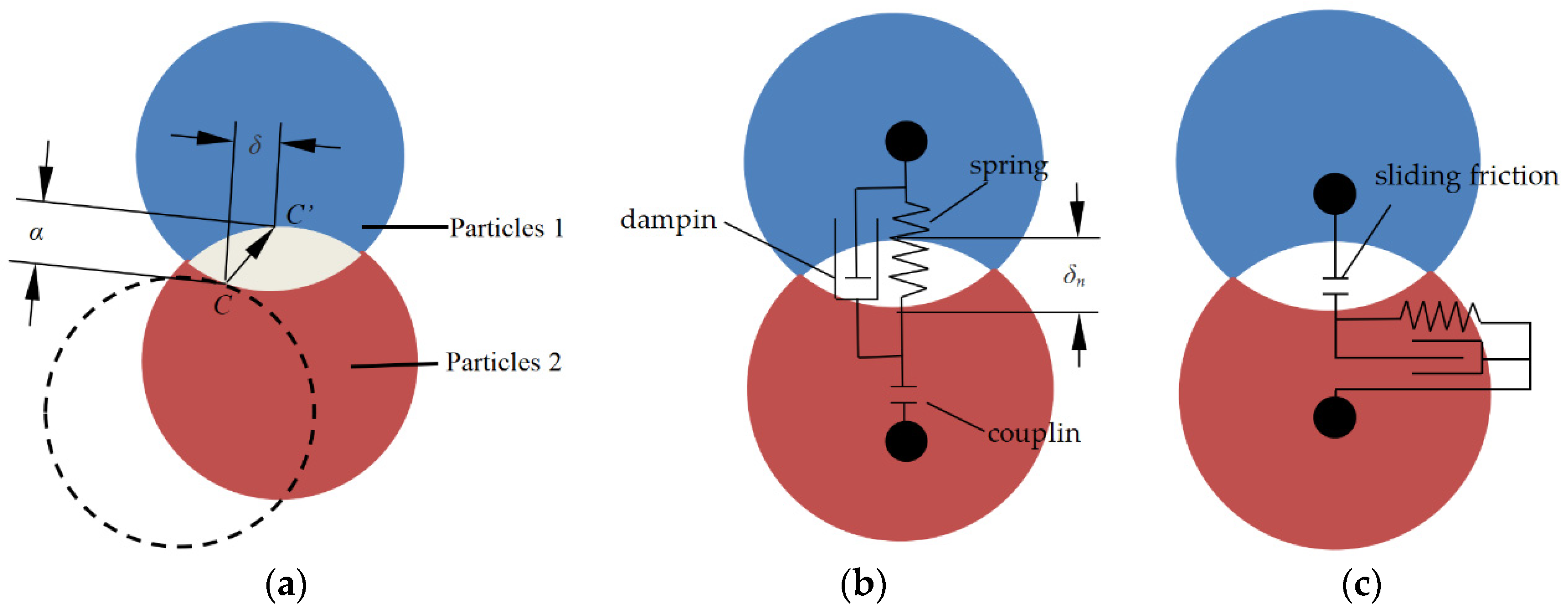
2.4.1. Contact Model
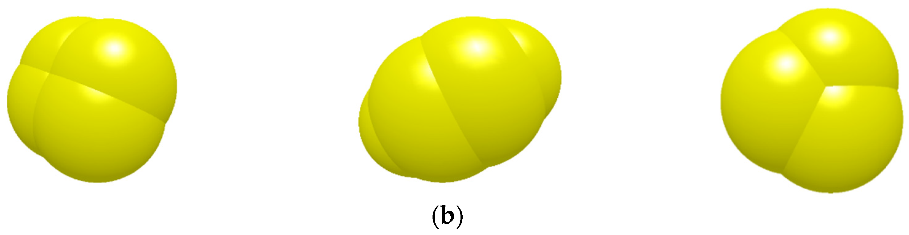
2.4.2. Discrete Elemental Modeling of Particles
2.4.3. Simulation Parameter Settings
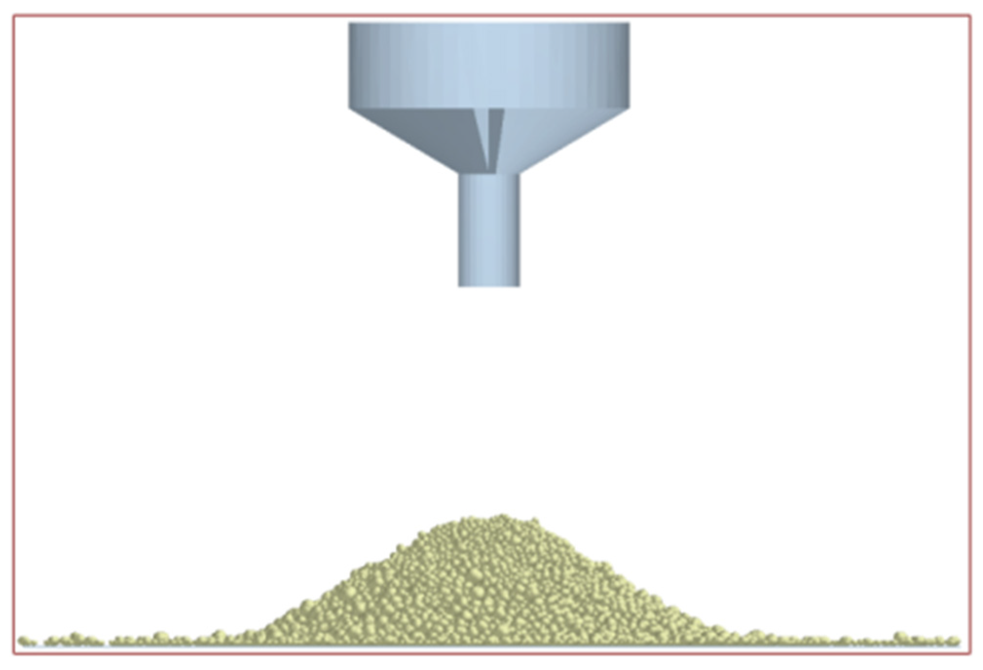
2.4.4. Stacking Simulation Model
3. Results and Discussion
3.1. PB Experimental Design
3.1.1. PB Experimental Design and Results
3.1.2. Analysis of PB Test Results
3.2. Steepest Climb Test
3.3. Response Surface Analysis Test
3.3.1. BBD Test Design and Results
3.3.2. Regression Model Analysis
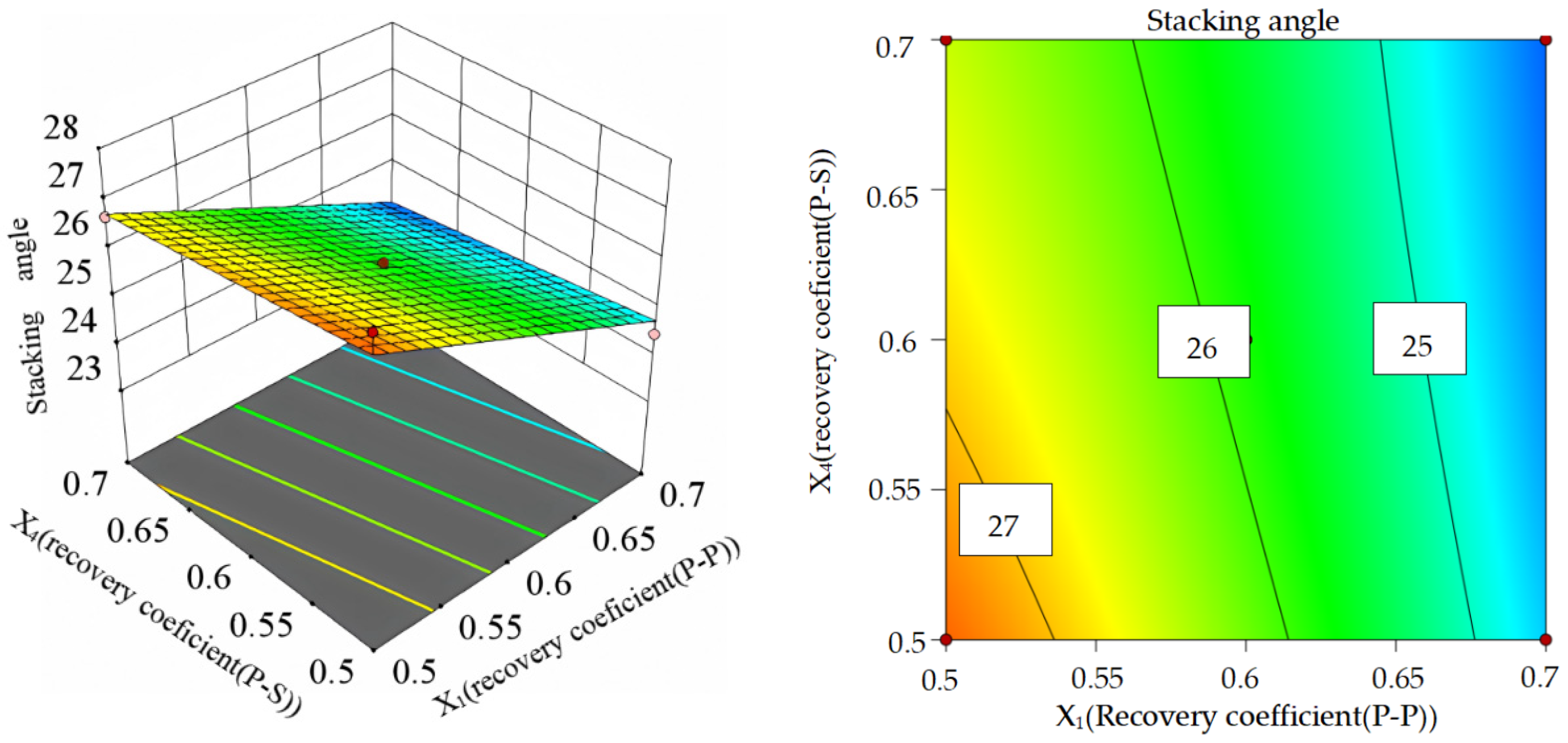
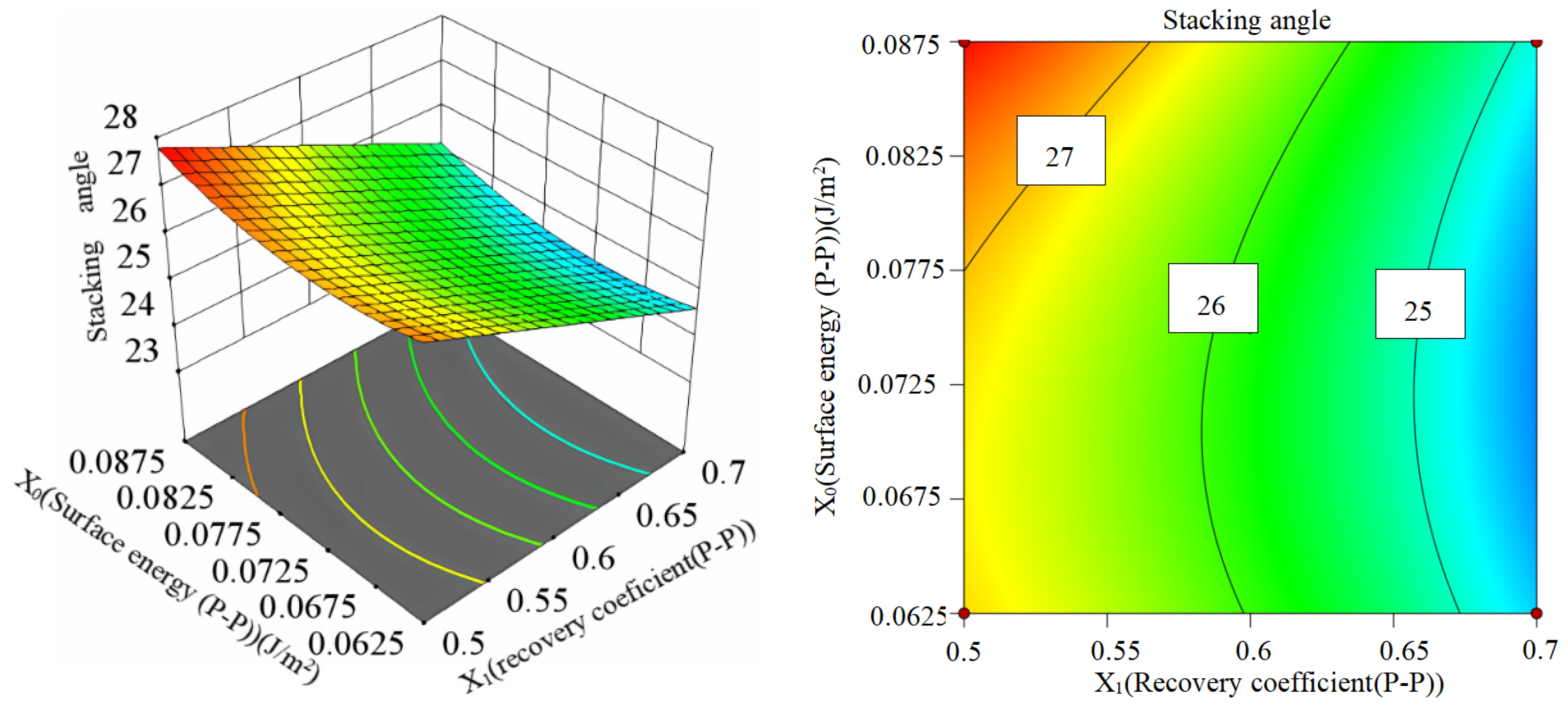
3.3.3. Analysis of Interaction Effects
3.4. Validation Experiments
4. Conclusions
- (1)
- This paper utilizes EDEM discrete element simulation software to specifically analyze the lees particles in a winery. The Hertz-Mindlin with JKR contact model is selected to simulate the lees particles with a moisture content of 20.4%. Through the screening process using Plackett-Burman Design, the contact parameters and model parameters that significantly affect the angle of repose of the lees particles were identified. The results indicated that the particle-particle coefficient of recovery and the particle-plate coefficient of recovery had the most significant impact.
- (2)
- The steepest climb test was employed to determine the optimal value ranges for significance parameters and surface energy. A regression model between the angle of repose of lees particles and these significance parameters as well as surface energy was established and optimized using the Box-Behnken Design response surface analysis test. Analysis of variance (ANOVA) revealed that, in addition to significance parameter and surface energy, the quadratic term of surface energy between particles also had a significant effect on the angle of repose of lees particles.
- (3)
- By taking into account the actual angle of repose as an objective response value, optimization and solution techniques were applied to obtain three optimal parameter values: a particle-particle recovery coefficient of 0.603, a particle-plate recovery coefficient of 0.595, and a JKR value of 0.083.
- (4)
- By substituting the optimal values of the discrete element parameters for the simulation test of the angle of repose of lees particles, it was found that the relative error with the experimental angle of repose is 0.18%. This result proves that the method of obtaining optimal parameter values by solving the angle of repose as the response value is effective. The comparative validation test results also demonstrate that there is no significant difference between the simulated rest angle of lees particles and the actual rest angle, thus confirming the accuracy and reliability of the calibrated discrete element model parameters for lees particles.
Author Contributions
Funding
Institutional Review Board Statement
Data Availability Statement
Conflicts of Interest
Appendix A

| Parameters | Sum of Mean Squares | Freedom | Mean Square | F | p | Significance |
|---|---|---|---|---|---|---|
| Models | 16.08 | 9 | 1.79 | 13.27 | 0.0054 | * |
| X1 | 13.44 | 1 | 13.44 | 99.88 | 0.0002 | * |
| X4 | 0.768 | 1 | 0.768 | 5.71 | 0.062 | |
| X0 | 0.612 | 1 | 0.612 | 4.54 | 0.086 | |
| X1X4 | 0.041 | 1 | 0.041 | 0.303 | 0.606 | - |
| X1X0 | 0.077 | 1 | 0.077 | 0.569 | 0.485 | - |
| X4X0 | 0.252 | 1 | 0.252 | 1.87 | 0.229 | - |
| X12 | 0.204 | 1 | 0.204 | 1.51 | 0.273 | - |
| X42 | 0.010 | 1 | 0.010 | 0.073 | 0.797 | - |
| X02 | 0.618 | 1 | 0.618 | 4.59 | 0.085 | |
| Residual | 0.673 | 5 | 0.135 | |||
| Lack of Fit | 0.673 | 3 | 0.224 | |||
| Pure error | 0 | 2 | 0 | |||
| Cor Total | 16.75 | 14 | ||||
| R2 = 0.9598, R2adj = 0.8875, CV = 1.41%, Adeq Precision = 11.9308 | ||||||
| Parameters | Sum of Mean Squares | Freedom | Mean Square | F | p | Significance |
|---|---|---|---|---|---|---|
| Models | 15.95 | 6 | 2.66 | 26.58 | <0.0001 | ** |
| X1 | 13.44 | 1 | 13.44 | 134.38 | <0.0001 | ** |
| X4 | 0.77 | 1 | 0.77 | 7.68 | 0.024 | * |
| X0 | 0.61 | 1 | 0.61 | 6.11 | 0.039 | * |
| X4X0 | 0.25 | 1 | 0.25 | 2.52 | 0.151 | - |
| X12 | 0.21 | 1 | 0.21 | 2.12 | 0.184 | - |
| X02 | 0.61 | 1 | 0.61 | 6.1 | 0.039 | * |
| Residual | 0.80 | 8 | 0.10 | |||
| Lack of Fit | 0.80 | 6 | 0.13 | |||
| Pure error | 0 | 2 | 0 | |||
| Cor Total | 16.75 | 14 | ||||
| R2 = 0.9522, R2adj = 0.9164, CV = 1.22%, Adeq Precision = 16.5885 | ||||||
| Parameters | Sum of Mean Squares | Freedom | Mean Square | F | p | Significance |
|---|---|---|---|---|---|---|
| Models | 15.95 | 4 | 3.87 | 30.62 | <0.0001 | ** |
| X1 | 13.44 | 1 | 13.44 | 106.30 | <0.0001 | ** |
| X4 | 0.77 | 1 | 0.77 | 6.08 | 0.033 | * |
| X0 | 0.61 | 1 | 0.61 | 4.84 | 0.053 | * |
| X02 | 0.67 | 1 | 0.67 | 5.26 | 0.045 | * |
| Residual | 1.26 | 10 | 0.13 | |||
| Lack of Fit | 1.26 | 8 | 0.16 | |||
| Pure error | 0 | 2 | 0 | |||
| Cor Total | 16.75 | 14 | ||||
| R2 = 0.9245, R2adj = 0.8943, CV = 1.37%, Adeq Precision = 17.5399 | ||||||
References
- Wang, X.; Jiang, Z.; Yang, J.; Qin, H.; Lei, L. Research Progress of Robot Steaming in Solid Baijiu Distillation. Liquor. Mak. 2024, 51, 32–35. [Google Scholar]
- Li, H.L.; Huang, W.X.; Yi, B.; Yang, J.; Yang, P. Ethanol/moisture contents in fermented grains and their effects on the yield and quality of Chinese Luzhou-flavor liquor. Adv. Mater. Res. 2012, 396, 1605–1610. [Google Scholar] [CrossRef]
- Li, H.; Huang, W.; Shen, C.; Yi, B. Optimization of the distillation process of Chinese liquor by comprehensive experimental investigation. Food Bioprod. Process. 2012, 90, 392–398. [Google Scholar] [CrossRef]
- Tian, W. Robot Design and Experimental Research Oriented to the Steam Detection and Steaming Process. Master’s Thesis, Sichuan University of Science & Engineering, Zigong, China, 2020. [Google Scholar] [CrossRef]
- Zhang, M.; Tang, Y.; Zhang, H.; Lan, H.; Niu, H. Parameter Optimization of Spiral Fertilizer Applicator Based on Artificial Neural Network. Sustainability 2023, 15, 1744. [Google Scholar] [CrossRef]
- Ji, J.; Jin, T.; Li, Q.; Wu, Y.; Wang, X. Construction of Maize Threshing Model by DEM Simulation. Agriculture 2024, 14, 587. [Google Scholar] [CrossRef]
- Mou, X.; Wan, F.; Wu, J.; Luo, Q.; Xin, S.; Ma, G.; Zhou, X.; Huang, X.; Peng, L. Simulation Analysis and Multiobjective Optimization of Pulverization Process of Seed-Used Watermelon Peel Pulverizer Based on EDEM. Agriculture 2024, 14, 308. [Google Scholar] [CrossRef]
- Li, D.; Wang, R.; Zhu, Y.; Chen, J.; Zhang, G.; Wu, C. Calibration of Simulation Parameters for Fresh Tea Leaves Based on the Discrete Element Method. Agriculture 2024, 14, 148. [Google Scholar] [CrossRef]
- Xu, B.; Zhang, Y.; Cui, Q.; Ye, S.; Zhao, F. Construction of a discrete element model of buckwheat seeds and calibration of parameters. INMATEH-Agric. Eng. 2021, 64, 175–184. [Google Scholar] [CrossRef]
- Wang, L.; Hu, C.; He, X.; Guo, W.; Wang, X.; Hou, S. A general modelling approach for coated cotton-seeds based on the discrete element method. INMATEH-Agric. Eng. 2021, 63, 221–230. [Google Scholar] [CrossRef]
- Balevičius, R.; Sielamowicz, I.; Mróz, Z.; Kačianauskas, R. Investigation of wall stress and outflow rate in a flat-bottomed bin: A comparison of the DEM model results with the experimental measurements. Powder Technol. 2011, 214, 322–336. [Google Scholar] [CrossRef]
- Grima, A.P.; Wypych, P.W. Development and validation of calibration methods for discrete element modelling. Granul. Matter 2011, 13, 127–132. [Google Scholar] [CrossRef]
- Santos, K.G.; Campos, A.V.P.; Oliveira, O.S.; Ferreira, L.V.; Francisquetti, M.C.; Barrozo, M.A.S. Dem simulations of dynamic angle of repose of acerola residue: A parametric study using a response surface technique. Blucher Chem. Eng. Proc. 2015, 1, 11326–11333. [Google Scholar]
- Xia, R.; Li, B.; Wang, X.; Li, T.; Yang, Z. Measurement and calibration of the discrete element parameters of wet bulk coal. Measurement 2019, 142, 84–95. [Google Scholar] [CrossRef]
- Gong, X.; Bai, X.W.; Huang, H.; Zhang, F.; Gong, Y.; Wei, D. Dem parameters calibration of mixed biomass sawdust model with multi-response indicators. INMATEH-Agric. Eng. 2022, 65, 183–192. [Google Scholar] [CrossRef]
- Michael, R.; Kevin, J.H. A methodical calibration procedure for discrete element models. Powder Technol. 2017, 307, 73–83. [Google Scholar] [CrossRef]
- Coetzee, C.J. Calibration of the discrete element method. Powder Technol. 2017, 310, 104–142. [Google Scholar] [CrossRef]
- Frączek, J.; Złobecki, A.; Zemanek, J. Assessment of angle of repose of granular plant material using computer image analysis. J. Food Eng. 2007, 83, 17–22. [Google Scholar] [CrossRef]
- Jia, F.; Han, Y.; Liu, Y.; Cao, Y.; Shi, Y.; Yao, L.; Wang, H. Simulation prediction method of repose angle for rice particle materials. Trans. Chin. Soc. Agric. Eng. (Trans. CSAE) 2014, 30, 254–260. [Google Scholar] [CrossRef]
- Favier, J.F.; Abbaspour-Fard, M.H.; Kremmer, M.; Raji, A.O. Shape representation of axi-symmetrical, non-spherical particles in discrete element simulation using multi-element model particles. Eng. Comput. 1999, 16, 467–480. [Google Scholar] [CrossRef]
- Abbaspour-Fard, M.H. Theoretical validation of a multi-sphere, discrete element model suitable for biomaterials handling simulation. Biosyst. Eng. 2004, 88, 153–161. [Google Scholar] [CrossRef]
- Kruggel-Emden, H.; Rickelt, S.; Wirtz, S.; Scherer, V. A study on the validity of the multi-sphere discrete element method. Powder Technol. 2008, 188, 153–165. [Google Scholar] [CrossRef]
- Yu, Y.; Zhou, H.; Fu, H.; Wu, X.; Yu, J. Modeling method of corn ears based on particles agglomerate. Trans. Csae 2012, 28, 167–174. (In Chinese) [Google Scholar] [CrossRef]
- Boac, J.M.; Casada, M.E.; Maghirang, R.G.; Harner, J.P. Material and interaction properties of selected grains and oilseeds for modeling discrete particles. Trans. Asabe 2010, 53, 1201–1216. [Google Scholar] [CrossRef]
- Weigler, F.; Mellmann, J. Investigation of grain mass flow in a mixed flow dryer. Particuology 2014, 12, 33–39. [Google Scholar] [CrossRef]
- Keppler, I.; Kocsis, L.; Oldal, I.; Farkas, I.; Csatar, A. Grain velocity distribution in a mixed flow dryer. Adv. Powder Technol. 2012, 23, 824–832. [Google Scholar] [CrossRef]
- Ramírez, A.; Nielsen, J.; Ayuga, F. On the use of plate-type normal pressure cells in silos: Part 2:Validation for pressure measurements. Comput. Electron. Agric. 2010, 71, 64–70. [Google Scholar] [CrossRef]
- Hu, J.; Xu, L.; Yu, Y.; Lu, J.; Han, D.; Chai, X.; Wu, Q.; Zhu, L. Design and Experiment of Bionic Straw-Cutting Blades Based on Locusta Migratoria Manilensis. Agriculture 2023, 13, 2231. [Google Scholar] [CrossRef]
- Xin, M.; Jiang, Z.; Song, Y.; Cui, H.; Kong, A.; Chi, B.; Shan, R. Compression Strength and Critical Impact Speed of Typical Fertilizer Grains. Agriculture 2023, 13, 2285. [Google Scholar] [CrossRef]


| Particle Radius Distribution/% | Densities/kg·m−3 | Poisson’s Ratio | Shear Modulus/Pa | ||
|---|---|---|---|---|---|
| ≤3.0 mm | 3.0–4.5 mm | ≧4.5 mm | |||
| 27.6% | 42.5% | 29.9% | 1053 | 0.4 | 1.1 × 10⁷ |
| EDEM Parameters | Materials | Value | Materials | Value |
|---|---|---|---|---|
| Density/kg·m−3 | Steel | 1930 | Particle | 1053 |
| Poisson’s ratio | Steel | 0.3 | Particle | 0.4 |
| Shear modulus/Pa | Steel | 2 × 10¹¹ | Particle | 1.1 × 10⁷ |
| Coefficient of restitution | Particle-steel | 0.4~0.8 | Particle-particle | 0.4~0.8 |
| Coefficient of static friction | Particle-steel | 0.5~1.0 | Particle-particle | 0.5~1.0 |
| Coefficient of rolling friction | Particle-steel | 0.01~0.02 | Particle-particle | 0.01~0.02 |
| Surface energy/J | Particle-particle | 0.05~0.1 |
| Surface Energy | Low Level | High Level |
|---|---|---|
| Particle-particle surface energy X0 | 0.05 | 0.1 |
| Particle-particle recovery coefficient X1 | 0.4 | 0.8 |
| Particle-particle static friction coefficient X2 | 0.5 | 1.0 |
| Particle-particle rolling friction coefficient X3 | 0.01 | 0.02 |
| Particle-steel coefficient of restitution X4 | 0.4 | 0.8 |
| Particle-steel static friction coefficient X5 | 0.5 | 1.0 |
| Particle-steel rolling friction coefficient X6 | 0.01 | 0.02 |
| Virtual factors V1, V2, V3, V4 | −1 | +1 |
| No. | X0 | X1 | V1 | X2 | X3 | V2 | X4 | X5 | V3 | X6 | V4 | Resting Angle/° |
|---|---|---|---|---|---|---|---|---|---|---|---|---|
| 1 | 0.1 | 0.4 | −1 | 1 | 0.02 | 1 | 0.8 | 0.5 | −1 | 0.01 | 1 | 27.0197 |
| 2 | 0.05 | 0.4 | −1 | 0.5 | 0.02 | 1 | 0.4 | 1 | 1 | 0.02 | 1 | 28.5799 |
| 3 | 0.1 | 0.4 | 1 | 1 | 0.02 | −1 | 0.4 | 1 | −1 | 0.02 | −1 | 28.679 |
| 4 | 0.05 | 0.8 | −1 | 1 | 0.01 | −1 | 0.8 | 1 | −1 | 0.02 | 1 | 13.5499 |
| 5 | 0.1 | 0.8 | −1 | 0.5 | 0.02 | −1 | 0.8 | 1 | 1 | 0.01 | −1 | 14.7664 |
| 6 | 0.1 | 0.4 | 1 | 0.5 | 0.01 | −1 | 0.8 | 0.5 | 1 | 0.02 | 1 | 25.4851 |
| 7 | 0.05 | 0.4 | −1 | 0.5 | 0.01 | −1 | 0.4 | 0.5 | −1 | 0.01 | −1 | 27.2393 |
| 8 | 0.05 | 0.8 | 1 | 1 | 0.02 | −1 | 0.4 | 0.5 | 1 | 0.01 | 1 | 22.2007 |
| 9 | 0.05 | 0.8 | 1 | 0.5 | 0.02 | 1 | 0.8 | 0.5 | −1 | 0.02 | −1 | 17.5636 |
| 10 | 0.05 | 0.4 | 1 | 1 | 0.01 | 1 | 0.8 | 1 | 1 | 0.01 | −1 | 25.9859 |
| 11 | 0.1 | 0.8 | −1 | 1 | 0.01 | 1 | 0.4 | 0.5 | 1 | 0.02 | −1 | 21.5922 |
| 12 | 0.1 | 0.8 | 1 | 0.5 | 0.01 | 1 | 0.4 | 1 | −1 | 0.01 | 1 | 22.6013 |
| Parameters | Effect | Sum of Mean Squares | Impact Rate | F | p | Significance Ranking |
|---|---|---|---|---|---|---|
| X0 | 0.84 | 2.10 | 0.70 | 0.42 | 0.55 | 4 |
| X1 | −8.45 | 214.33 | 70.97 | 42.38 | 0.00 | 1 |
| X2 | 0.47 | 0.65 | 0.22 | 0.13 | 0.74 | 6 |
| X3 | 0.39 | 0.46 | 0.15 | 0.09 | 0.78 | 7 |
| X4 | −4.42 | 58.62 | 19.41 | 11.59 | 0.03 | 2 |
| X5 | −1.16 | 4.01 | 1.33 | 0.79 | 0.42 | 3 |
| X6 | −0.73 | 1.59 | 0.53 | 0.31 | 0.61 | 5 |
| R2 = 0.9330, R2adj = 0.8158, CV = 9.8%, Adeq Precision = 7.7831 | ||||||
| No. | 1 | 2 | 3 | 4 | 5 |
|---|---|---|---|---|---|
| X0 | 0.05 | 0.0625 | 0.075 | 0.0875 | 0.1 |
| X1 | 0.8 | 0.7 | 0.6 | 0.5 | 0.4 |
| X2 | 0.75 | 0.75 | 0.75 | 0.75 | 0.75 |
| X3 | 0.015 | 0.015 | 0.015 | 0.015 | 0.015 |
| X4 | 0.8 | 0.7 | 0.6 | 0.5 | 0.4 |
| X5 | 0.75 | 0.75 | 0.75 | 0.75 | 0.75 |
| X6 | 0.015 | 0.015 | 0.015 | 0.015 | 0.015 |
| Resting angle/° | 17.89 | 23.8161 | 26.51365 | 27.3669 | 28.4261 |
| Relative error | 30.64% | 7.67% | 2.79% | 6.10% | 10.21% |
| Symbolic | Simulation Parameters | Low Level (−1) | Mid-Level (0) | High Level (1) |
|---|---|---|---|---|
| X0 | Particle-particle surface energy | 0.0625 | 0.075 | 0.0875 |
| X1 | Particle-particle recovery coefficient | 0.5 | 0.6 | 0.7 |
| X4 | Particle-steel recovery coefficient | 0.5 | 0.6 | 0.7 |
| No. | X0 | X1 | X4 | Resting Angle/° | Relative Error |
|---|---|---|---|---|---|
| 1 | −1 | −1 | 0 | 26.60 | 3.13% |
| 2 | 0 | 1 | −1 | 24.46 | 5.18% |
| 3 | 0 | −1 | 1 | 26.66 | 3.35% |
| 4 | 0 | 0 | 0 | 25.84 | 0.18% |
| 5 | 1 | 0 | 1 | 26.11 | 1.23% |
| 6 | 0 | 0 | 0 | 25.84 | 0.18% |
| 7 | 1 | 1 | 0 | 25.15 | 2.49% |
| 8 | −1 | 0 | −1 | 25.99 | 0.76% |
| 9 | −1 | 1 | 0 | 24.79 | 3.89% |
| 10 | 0 | 1 | 1 | 23.76 | 7.87% |
| 11 | 1 | −1 | 0 | 27.52 | 6.69% |
| 12 | −1 | 0 | 1 | 26.15 | 1.37% |
| 13 | 0 | 0 | 0 | 25.84 | 0.18% |
| 14 | 1 | 0 | −1 | 26.96 | 4.52% |
| 15 | 0 | −1 | −1 | 27.75 | 7.60% |
| Parameters | Values |
|---|---|
| Particle Poisson’s ratio | 0.4 |
| Particle shear modulus | 1.1 × 10⁷ Pa |
| Particle density | 1053 kg/m3 |
| Particle-particle recovery factor | 0.603 |
| Particle-particle static friction coefficient | 0.75 |
| Particle-particle rolling friction coefficient | 0.015 |
| Particle-steel recovery factor | 0.595 |
| Particle-steel static friction coefficient | 0.75 |
| Particle-steel rolling friction coefficient | 0.015 |
| Surface energy | 0.083 |
Disclaimer/Publisher’s Note: The statements, opinions and data contained in all publications are solely those of the individual author(s) and contributor(s) and not of MDPI and/or the editor(s). MDPI and/or the editor(s) disclaim responsibility for any injury to people or property resulting from any ideas, methods, instructions or products referred to in the content. |
© 2024 by the authors. Licensee MDPI, Basel, Switzerland. This article is an open access article distributed under the terms and conditions of the Creative Commons Attribution (CC BY) license (https://creativecommons.org/licenses/by/4.0/).
Share and Cite
Zhang, X.; Wang, R.; Wang, B.; Chen, J.; Wang, X. Parameter Calibration of Discrete Element Model of Wine Lees Particles. Appl. Sci. 2024, 14, 5281. https://doi.org/10.3390/app14125281
Zhang X, Wang R, Wang B, Chen J, Wang X. Parameter Calibration of Discrete Element Model of Wine Lees Particles. Applied Sciences. 2024; 14(12):5281. https://doi.org/10.3390/app14125281
Chicago/Turabian StyleZhang, Xiaoyuan, Rui Wang, Baoan Wang, Jie Chen, and Xiaoguo Wang. 2024. "Parameter Calibration of Discrete Element Model of Wine Lees Particles" Applied Sciences 14, no. 12: 5281. https://doi.org/10.3390/app14125281
APA StyleZhang, X., Wang, R., Wang, B., Chen, J., & Wang, X. (2024). Parameter Calibration of Discrete Element Model of Wine Lees Particles. Applied Sciences, 14(12), 5281. https://doi.org/10.3390/app14125281