Applicability of Digital Image Photogrammetry to Rapid Displacement Measurements of Structures in Restricted-Access and Controlled Areas: Case Study in Korea

Abstract

Critical facilities are generally located in areas with restricted or controlled access, making it difficult for experts to monitor the structural health of enclosed infrastructures. Hence, a case study was conducted in South Korea to evaluate the applicability of digital image photogrammetry using commercial imaging devices in order to quickly measure the structural deformations of infrastructures in such areas. The applicability evaluation involved measuring the displacement of mechanically stabilized earth (MSE) walls. In the experiment, the displacement of MSE walls was first measured using the traditional monitoring method and the results were compared with those obtained via digital image photogrammetry using commercial imaging devices such as digital cameras and cellphones. The measurement results obtained with the cellphone camera had a maximum error of approximately 20 mm when compared with the results of the traditional monitoring method. Because this is a significant error, even when considering the mechanical error in the traditional monitoring method’s result, it was determined that monitoring using a cellphone camera is infeasible. However, the experimental results of digital image photogrammetry using a digital camera showed a maximum error of approximately 9 mm. Although this is a sizable error, the method was assessed to be technically feasible.

1. Introduction

Most countries have established restricted-access and controlled areas for critical facilities. Such areas include not only critical structures such as power generation facilities but also the necessary infrastructure for securing the area. The infrastructure must be both economical and reliable, necessitating the continuous monitoring of its long-term behavior. Due to its national situation, South Korea has many areas with controlled or restricted-access. This makes the monitoring of the enclosed infrastructures by experts challenging due to time constraints and concerns related to monitoring accuracy. Therefore, it is necessary to find a way for non-experts to have free access to utilize the restricted-access or controlled area to monitor the infrastructure.

Mechanically stabilized earth walls (MSE walls) are representative structures in restricted-access and controlled areas. MSE walls are based on the principle of reinforced earth; i.e., reinforced earth increases the shear strength of the ground because the interaction between the soil and highly tensile reinforcement inhibits ground deformation due to an increase in the internal friction angle, the development of adhesion forces, and an increase in confining stresses [1,2]. MSE walls are preferred for securing the stability of various structures, such as slopes, bridges, roads, etc., due to their economic construction and high field applicability [3,4,5,6,7,8,9]. Hence, MSE walls are commonly found worldwide [10,11,12,13]. In the past, South Korea primarily used reinforced concrete walls to secure important facilities. However, due to their superior applicability, the construction of MSE walls has increased rapidly since the 1990s. In particular, the scale of MSE walls has increased due to the securing of more effective sites and the enlargement of facilities, and they are increasingly constructed using facing blocks.

An MSE wall consists of wall facings, reinforcements, and backfill soil. The wall facing not only forms the appearance of the MSE wall but also prevents the loss of backfill soil. Generally, wall facing is applied to panels or blocks. Reinforcements are divided into non-extensible and extensible reinforcements according to the material properties. Non-extensible reinforcements include smooth steel strips, ribbed steel strips, and steel grids. Elastic reinforcements include geosynthetics, such as geogrids and geotextiles. The reinforcement interacts with the backfill soil to form the reinforced earth zone of the MSE wall [12,13].

The design of the MSE walls is evaluated for both external and internal stability. The external stability assessment considers the reinforced earth as an integral structure and applies the same concepts as those applied in the stability of a gravity-retaining wall, i.e., base sliding, overturning, and bearing capacity. Internal stability is evaluated in terms of slip failure, pullout of reinforcement, and tensile overstress. In addition, global stability, including that of reinforced earth, is considered if the MSE wall is applied to a slope or if there is a high embankment slope behind the MSE wall [1,2,14,15,16,17,18]. When problems arise with the external, internal, and global stability of a constructed MSE wall, obvious symptoms emerge, such as cracking and the settlement of the wall facing. However, as with all infrastructure, following stabilization, MSE walls can develop structural instability over time, necessitating ongoing maintenance. In particular, damage to the MSE walls is very difficult to repair due to their structural characteristics, which require fast, economical, and reliable detection and monitoring [12,13].

The maintenance of structures is dominated by traditional and passive surface monitoring instrumentation methods, such as inclinometers, displacement meters, crack gauges, and total stations. Despite the high accuracy of passive instruments, such as total stations, it is almost impossible to measure the behavior of civil structures in real time due to variations in the site’s conditions. Furthermore, conventional photogrammetry requires time-consuming analyses of the measured data because it involves taking pictures, drawing, and analyzing the data. Accordingly, many studies have recently been conducted on the application of digital monitoring methods and automatic measurement methods in various industries [19,20,21,22].

The monitoring of MSE walls is mostly based on manual and visual field inspections using basic devices such as inclinometers. This leads to irregularities in the reliability of the results, depending on the expertise of the person performing the measurement [12,23,24,25,26]. Various devices such as global positioning systems and total stations are widely used to measure the deformation and inclination of MSE walls, but they have many limitations in terms of time and physical accessibility [27,28,29,30].

Researchers have extensively studied the use of scanning techniques in conjunction with digital image photogrammetry. In particular, remote sensing techniques are becoming popular for monitoring infrastructures such as MSE walls [23,31,32,33]. Typical remote sensing techniques for monitoring structures include light detection and ranging (LiDAR), laser scanning (terrestrial), and synthetic aperture radar [23]. However, these techniques always have limitations, such as atmospheric conditions, the acquisition of measurement targets, and satellite access [34,35,36,37].

Laefer and Lennon [38] investigated the use of terrestrial laser scanning to monitor retaining walls with precast concrete panels. They concluded that the deformation of the MSE wall facing can be identified by analyzing multi-temporal scans. Oskouie et al. [10] used terrestrial laser scanning to obtain the point clouds of MSE walls. They then checked the monitoring potential using a flat model from which extraneous objects had been removed. The random sample consensus (RANSAC) algorithm [39] was used in the study. Lin et al. [40] evaluated the tilts and movements of MSE walls with panels using terrestrial laser scanning. Lienhart et al. [41] proposed a practical monitoring approach using a mobile mapping system for monitoring earth walls, but their results were limited to the transversal tilt angle. Aldosar et al. [13] proposed a monitoring method for MSE walls with panels using mobile LiDAR.

Digital image photogrammetry has the advantage of being able to obtain three-dimensional coordinates, which makes it possible to automatically determine the behavior of measurement points. In particular, the stability assessment of large civil engineering structures increasingly employs automated measurement systems based on digital image photogrammetry. The digital image photogrammetry procedure involves image acquisition, image processing, and analyses of the target object. Traditionally, photogrammetry has been analyzed using film-based image acquisition, but CCD and CMOS cameras have been recently applied. The scale and pixel size of the images based on CCD and CMOS cameras are important factors in image analysis for digital image photogrammetry, i.e., improving the accuracy of the image has a significant effect on the measurement results [42]. Therefore, the distortion correction of the camera lens may be necessary for improving the accuracy of geometric variables in digital images [42].

The continuous development of optical cameras, image processing, and 3D modeling technologies has made it easy to implement 3D models from 2D images based on digital image photogrammetry [43,44,45,46]. This implies that 3D models constructed from 2D images can yield quantitative localization information. Thus, many physical constraints in the monitoring of the deformation of MSE walls can be solved. Nevertheless, the research on the application of digital image photogrammetry to the monitoring of MSE walls is relatively limited.

This study aims to determine whether digital image photogrammetry equipment, including a digital camera and commercial program, can accurately measure the MSE wall deformation in areas with restricted-access and security due to the current situation in South Korea. The applicability evaluation was conducted by comparing and analyzing the measurement results of traditional monitoring and digital image photogrammetry methods for MSE wall displacement in restricted-access and controlled areas. That is, this study consists of field investigations, monitoring results and analyses, error rate evaluations, and discussions, and the experimental study was conducted using the following methodology. The electrical resistivity survey was conducted to evaluate the cause of the displacement of the MSE wall, and the monitoring target location was determined from the results. Then, the monitoring of the MSE wall using the traditional monitoring method and digital image photogrammetry was conducted. In addition, the displacement facing the MSE wall was analyzed using the monitoring results, and the error was evaluated. Finally, the limitations of this study and the need for additional research were suggested based on the error rate analysis results. The results are directed toward increasing the utility of the applied technology by enabling rapid measurements of infrastructure in areas with very limited access.

2. Materials and Methods

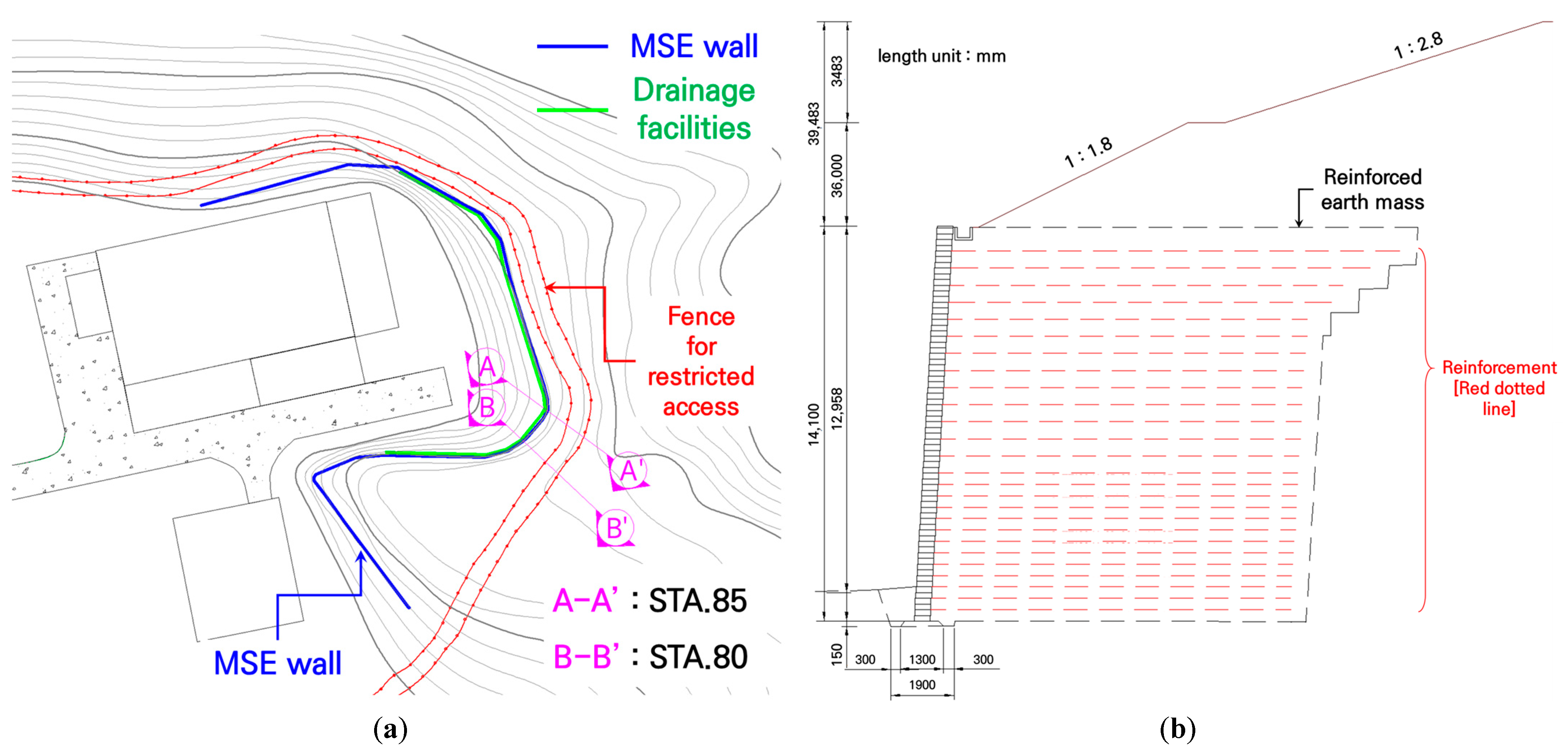
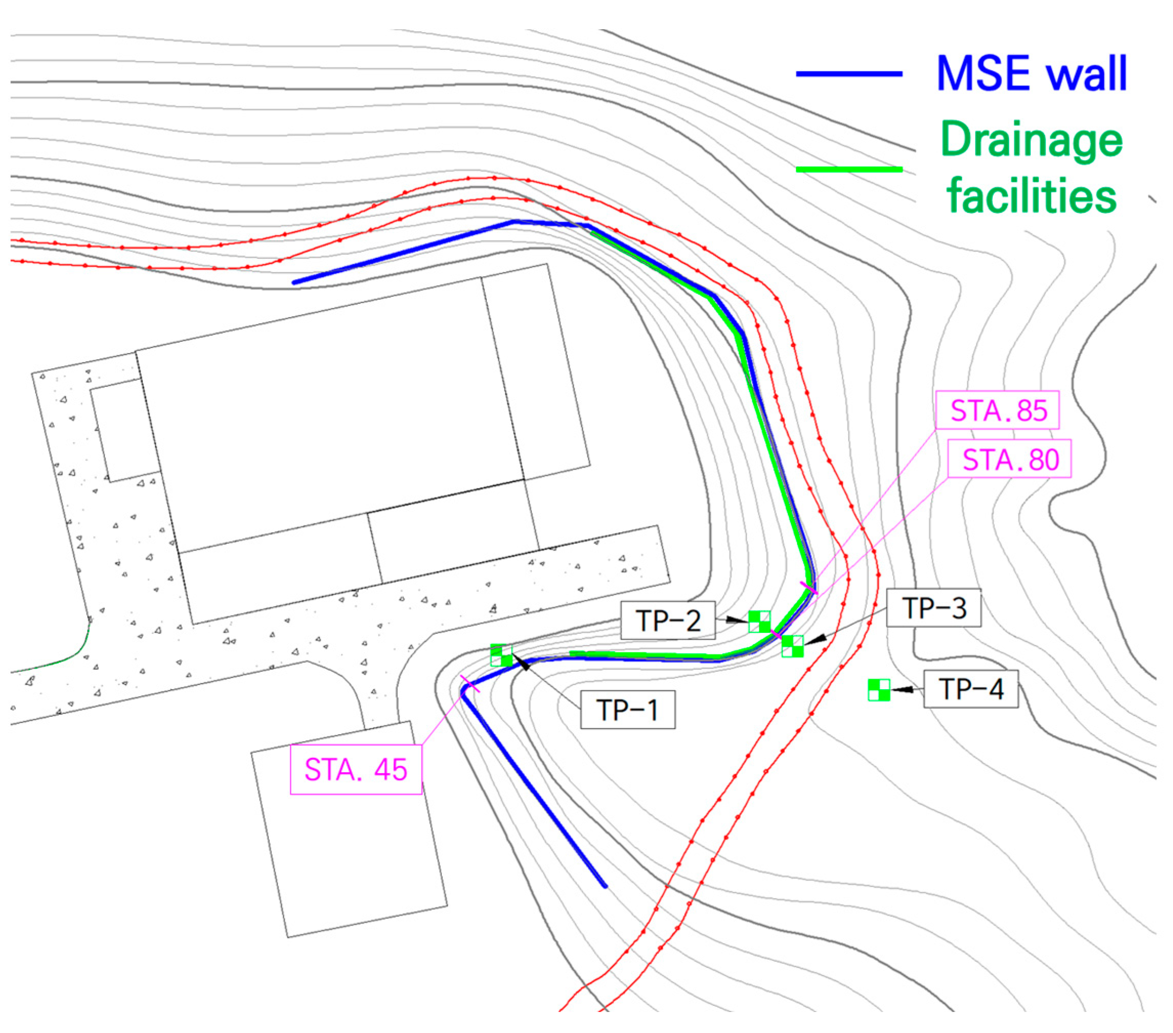
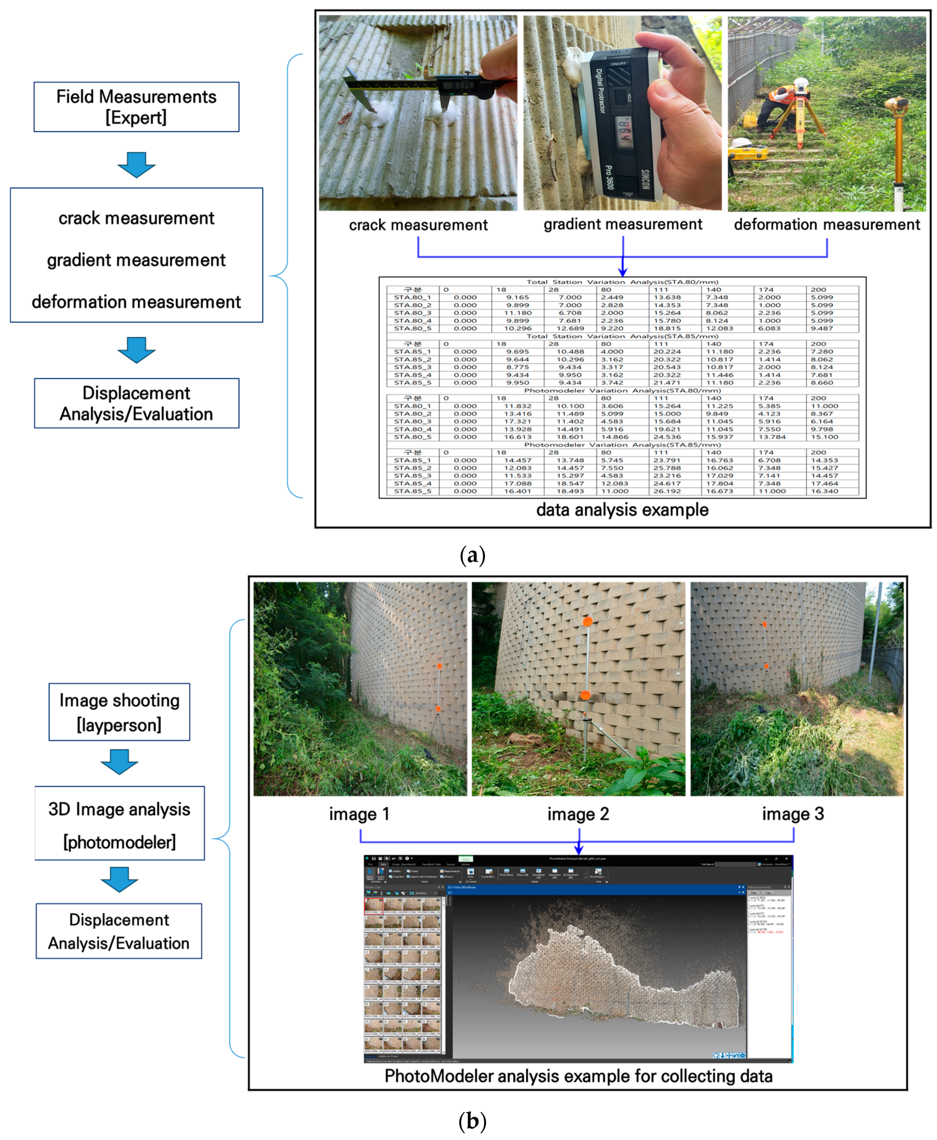
2.1. Field Investigation

The MSE wall under study was constructed in 2005 to secure a site on the backside and extends 211 m. A longitudinal crack deformed the corner height of the MSE wall by 14.1 m. The longitudinal crack-affected section was managed through displacement measurements. Figure 1 shows the construction plan and cross-sectional view of the MSE wall displacement section.

An investigation was conducted to determine the cause of the longitudinal cracking at the MSE wall’s corners. Drilling and electrical resistivity surveys were conducted on the MSE wall backfill and the underlying subgrade to distinguish between a straight section with no cracks and a corner with multiple longitudinal cracks. The straight section and corner were surveyed at STA.45 and STA.80, respectively, and the geotechnical survey was conducted at a depth of less than 1 m. ‘STA(Station)’ refers to a measurement word used to indicate a specific survey location on a drawing. Figure 2 presents the geotechnical survey plan, and

Table 1. Geotechnical survey contents.

Separation	Depth of Investigation (m)	Ground Layer	Remarks
TP-1	0.0 to 0.8	Reclaimed soil layers	Straight
TP-2	0.0 to 1.0		Corner (top)
TP-3	0.0 to 0.5		Corner (bottom)
TP-4	0.0 to 0.3	Topsoil layer	Original ground

shows the geotechnical survey depths for each survey location.

The results of the ground investigation confirmed that layers from TP-1 to TP-3 were reclaimed soil layers and TP-4 was a topsoil layer. The soil type of TP-1 and TP-2 sites were identified as silty sand with gravel, and TP-3 as clay with gravel. Moreover, the soil type of the TP-4 site comprised low-plasticity clay with sand.

Table 2. Engineering properties of soils.

Separation	wn (%)	Gs	Atterberg Limits		Grain Size Distribution (%)					USCS	Total Unit Weight (${\mathit{\gamma }}_{\mathit{t}},\mathbf{k}\mathbf{N}/{\mathbf{m}}^3$)	Dry Unit Weight (${\mathit{\gamma }}_{\mathit{d}},\mathbf{k}\mathbf{N}/{\mathbf{m}}^3$)
			LL (%)	PI (%)	#4 (4.75 mm)	#10 (2.00 mm)	#40 (0.425 mm)	#200 (0.075 mm)	0.005 mm
TP-1	12.1	2.67	-.	NP	62.4	49.4	34.5	20.1	4.5	SM	19.94	17.79
TP-2	20.9	2.68	31.4	5.6	83.0	75.0	65.3	43.2	9.5	SM	19.95	16.50
TP-3	18.5	2.67	32.4	9.9	49.0	43.7	36.5	29.9	11.5	GC	22.41	18.91
TP-4	28.1	2.68	40.8	18.2	100.0	100.0	90.6	70.4	23.0	CL	18.58	14.50

shows the engineering properties of each investigated site.

The electrical resistivity survey was conducted to determine the condition of the reinforced earth mass of the MSE wall. An electrical resistivity survey is a common non-destructive exploration technique used to determine the condition of the ground by measuring the potential difference caused by the difference in electrical resistivity among the differences in underground electrical properties. The electrical resistivity survey instrument supplies power to two current electrodes through an ammeter connected to a power source. It works on the principle that the potential difference is measured using an electrometer connected to two other potential electrodes through the supplied current. In this research, the electrode spacing of the electrical resistivity survey was installed at 5.0 m in order to consider the exploration depth and exploration extension of the ground. In addition, the ground condition was evaluated to identify leakage and problem areas distributed inside and around the MSE wall. The instrument used for the electrical resistivity survey is shown in Figure 3.

Figure 4 shows the electrical resistivity survey location plan of the case study’s site. As shown in Figure 4, four zones were surveyed at the top and bottom of the MSE wall from the ER-1-1 line to the ER-2-3 line. ER-1 and ER-2 lines refer to the exploration of the original ground and backing ground in front of the MSE wall, respectively.

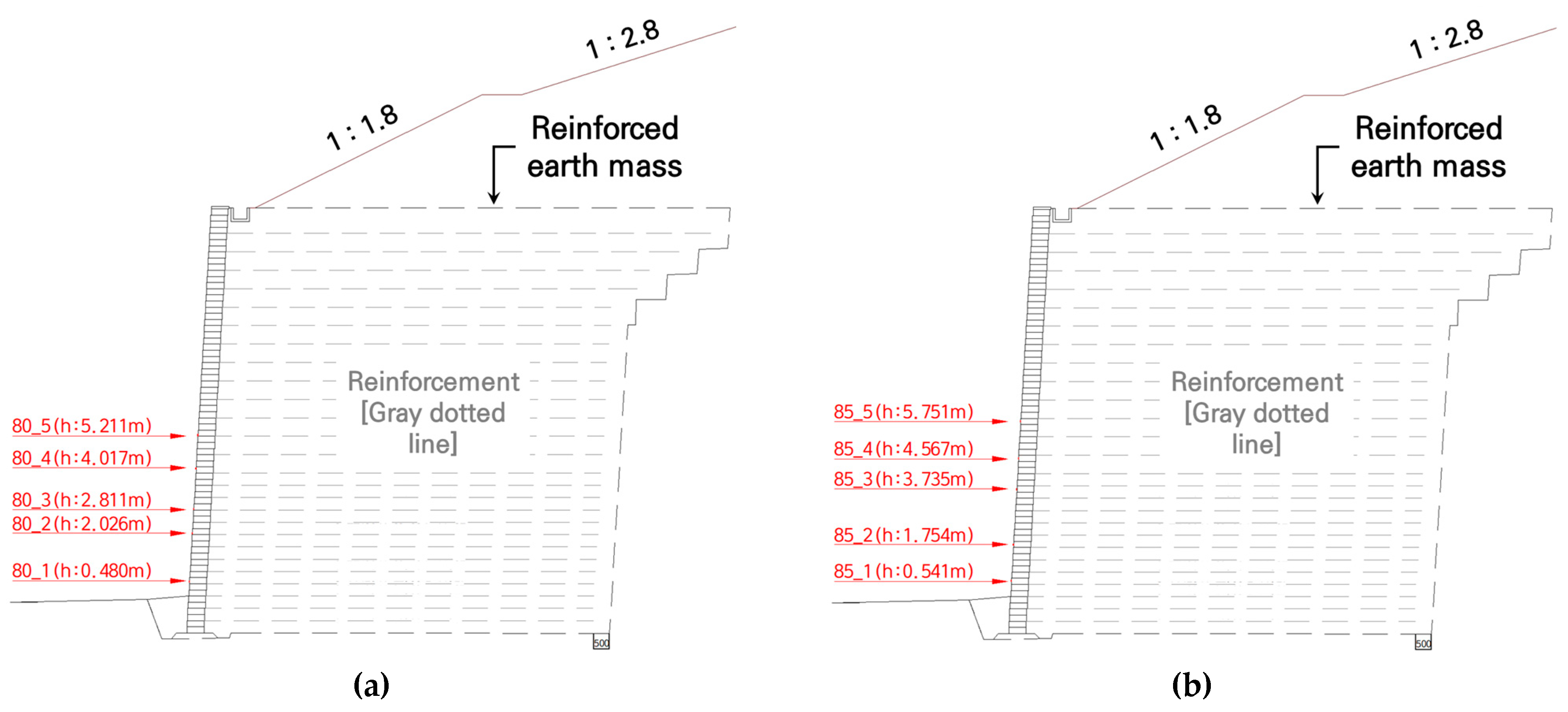
2.2. Monitoring of the MSE Wall

As mentioned above, the traditional monitoring method for MSE walls is to conduct onsite measurements of structural deformations using inclinometers, crack meters, and total stations at regular intervals, followed by internal office work management. However, the traditional monitoring method has limitations, such as the necessity of checking the structural deformation, which is the premise of the structure, due to the local measurement management of the MSE wall; restrictions with respect to measurement heights to ensure the stability of the operator; and the necessity of performing measurements, which are carried out by equipment experts. In particular, because many restricted-access and controlled areas in South Korea are located in mountainous and remote areas, the MSE walls are not accessible to experts on the site. The reliability of measurement results is also often challenged by the time constraints required to monitor the structure. Therefore, a method for monitoring the MSE walls by laypersons residing in the restricted-access and controlled areas is needed. This study employed digital image photogrammetry to assess the deformation of MSE walls. Figure 5 shows a comparison of the traditional monitoring and digital image photogrammetry procedures for MSE walls.

In this study, a total station is used for the traditional monitoring method, and it is generally applied to the measurement of structural surface displacements. A total station is an electronic device that can measure three-dimensional positions in space using light waves such as lasers. It requires a reflective target for the accurate measurement of a specific position and has high mechanical reliability. However, experts are required for measurement, and the reliability of the measurement results may vary depending on the expert. Digital image photogrammetry applied in this research can acquire images using imaging devices such as digital cameras and cellphone cameras, and it can measure the displacement of a required position in the image using a 3D analysis program.

The digital image photogrammetry procedure based on commercial imaging devices is summarized as follows. First, the surface of the MSE wall is photographed using a digital camera or cellphone camera and sent to a remote expert. The expert then uses a 3D image conversion program (PhotoModeler) to check the wall displacement of the MSE wall. In comparison with the traditional monitoring method, this approach has advantages, such as time-saving qualities and high applicability, as the image can be taken by laypersons. In other words, it is a very simple monitoring method that allows laypersons in restricted-access and controlled areas to take multiple images of the target structure using commercial imaging devices, and they can send them to experts at a remote location.

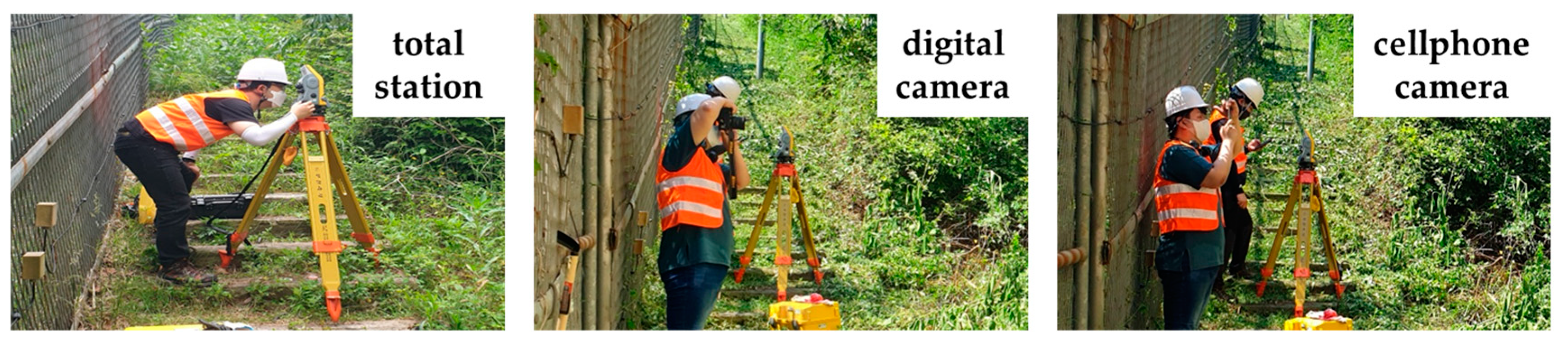
2.3. Displacement Measurement Field Experiment on MSE Wall

A field experiment was conducted on a case site to compare the traditional monitoring method (total station measurement) and digital image photogrammetry using commercial imaging devices. As shown in Figure 1a, the field experiment was conducted at the corners (STA.80 and STA.85) bearing the longitudinal cracks. For measurement and monitoring, traditional monitoring methods and digital image photogrammetry (digital camera) were carried out for 7 months, and digital image photogrammetry (cellphone camera) was used for 4 months. Figure 6 shows the locations of the wall deformation measurements on the MSE wall.

The field experiment process can be summarized as follows.

The traditional monitoring method using total stations utilizes a reflection target on a specific surface of the MSE wall corresponding to the measurement location. Then, internal office work on the analysis of position changes is performed in the office, after obtaining 3D coordinates through the measurement of the reflection target by an expert. Digital image photogrammetry uses digital cameras and cellphone cameras, and it acquires two or more MSE wall images of the measurement target from each device. The acquired images are immediately transmitted to the PhotoModeler operator in the office via wireless Internet, and the operator performs image alignment, camera calibration, and 3D position information analyses. Since the use of PhotoModeler requires images, it is only used for digital image photogrammetry. In digital image photogrammetry, the image acquisition location can affect the error in the results of two or more image registrations. Therefore, the digital camera and cellphone camera locations were maintained at ±45° from the front of the measurement location, and they were placed within approximately 10 to 15 m from the measurement location. Figure 7 displays the field experiment.

The field experiment employed a C3 total station manufactured by Trimble Inc., (Westminster, CO, USA). The specifications of Trimble C3 were 800 m and 3.0 mm + 2 ppm for the measurement distance and accuracy without reflective targets, respectively. With the prism, the measurement distance and accuracy were 5000 m and 2.0 mm + 2 ppm, respectively. The digital camera used was D7100, which has a CMOS sensor manufactured by Nikon (Tokyo, Japan). The D7100 has 24,710,000 pixels. The cellphone camera was a Galaxy S21 model from Samsung Electronics (Seoul, Republic of Korea) with 12 million pixels.

3. Results and Discussion

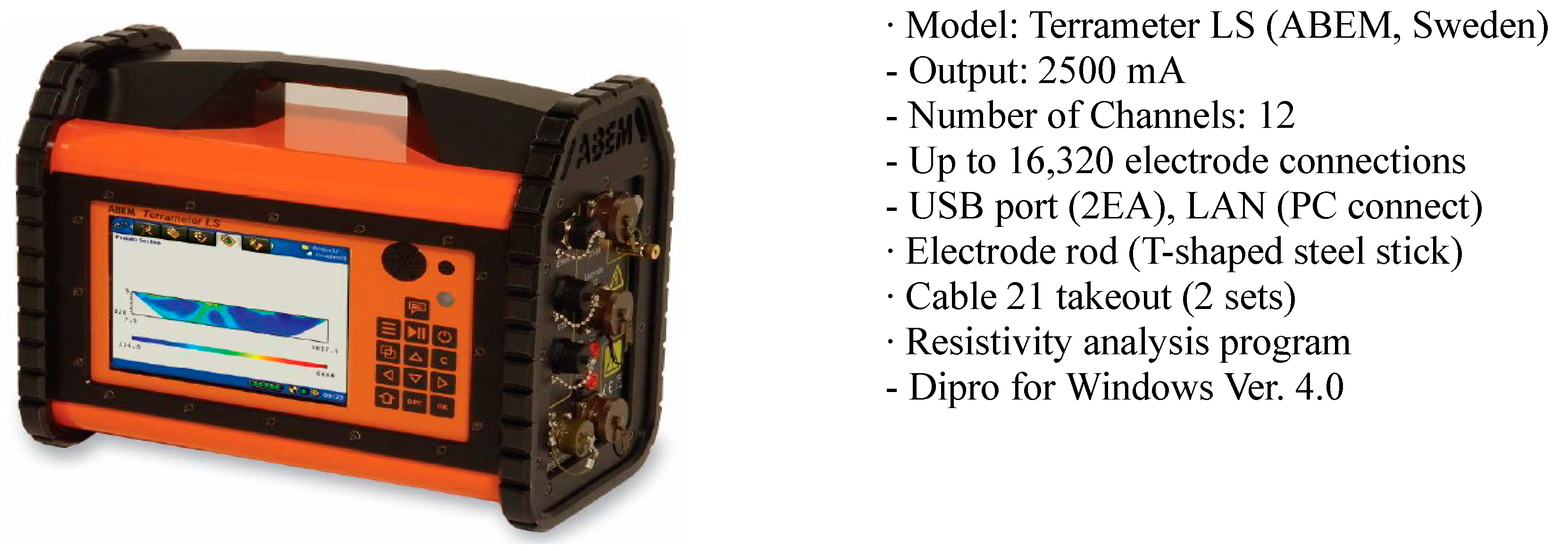
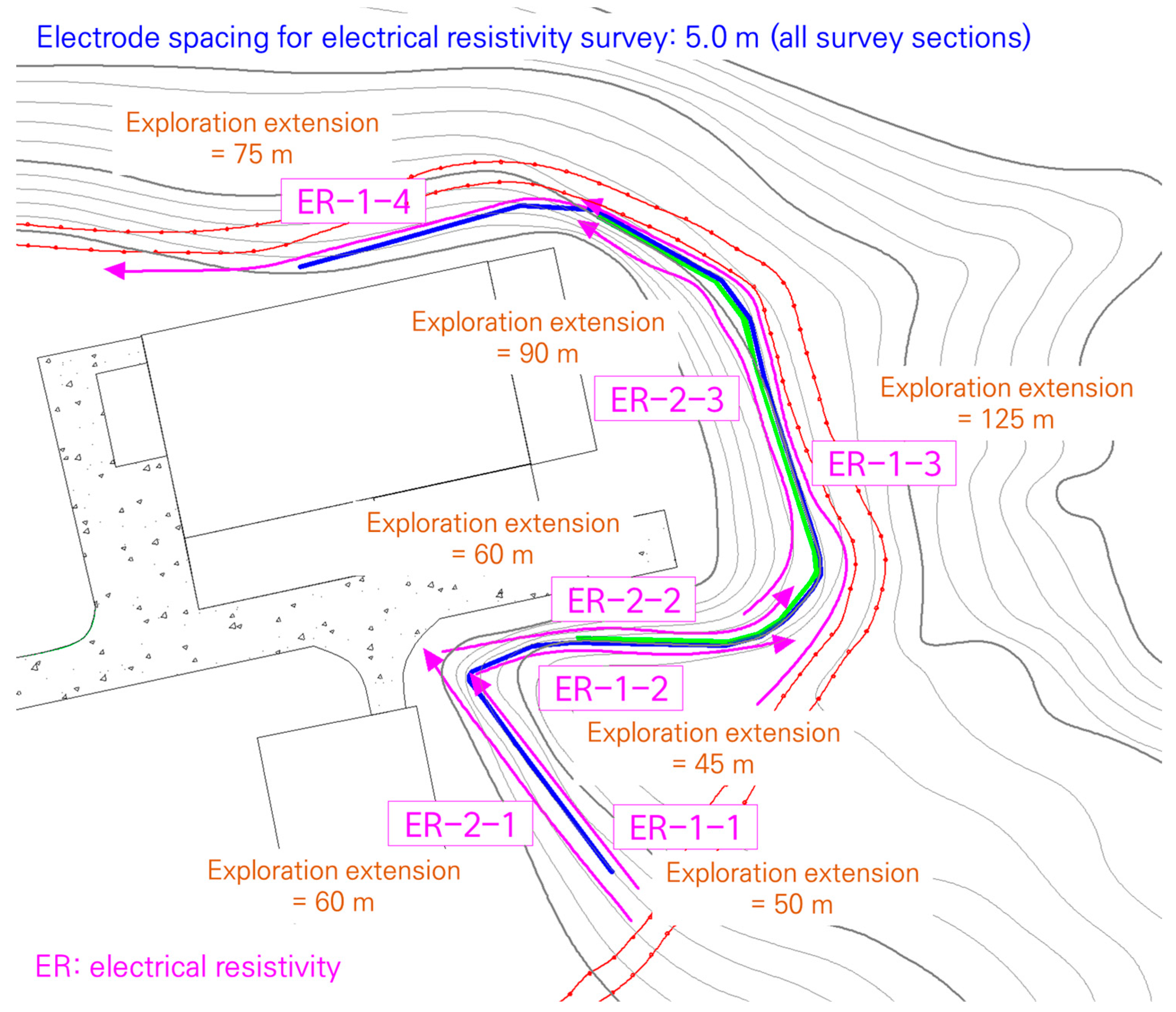
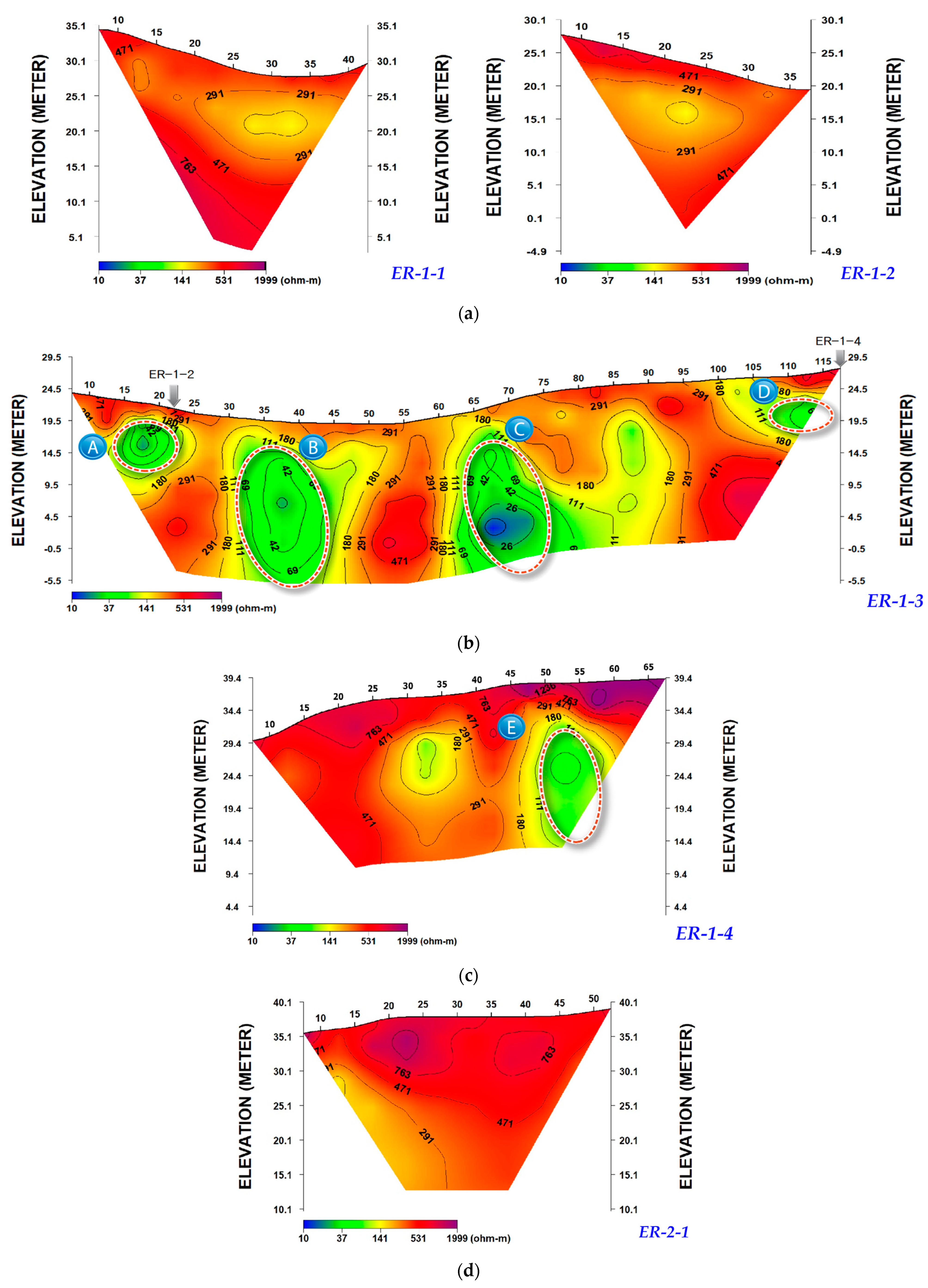
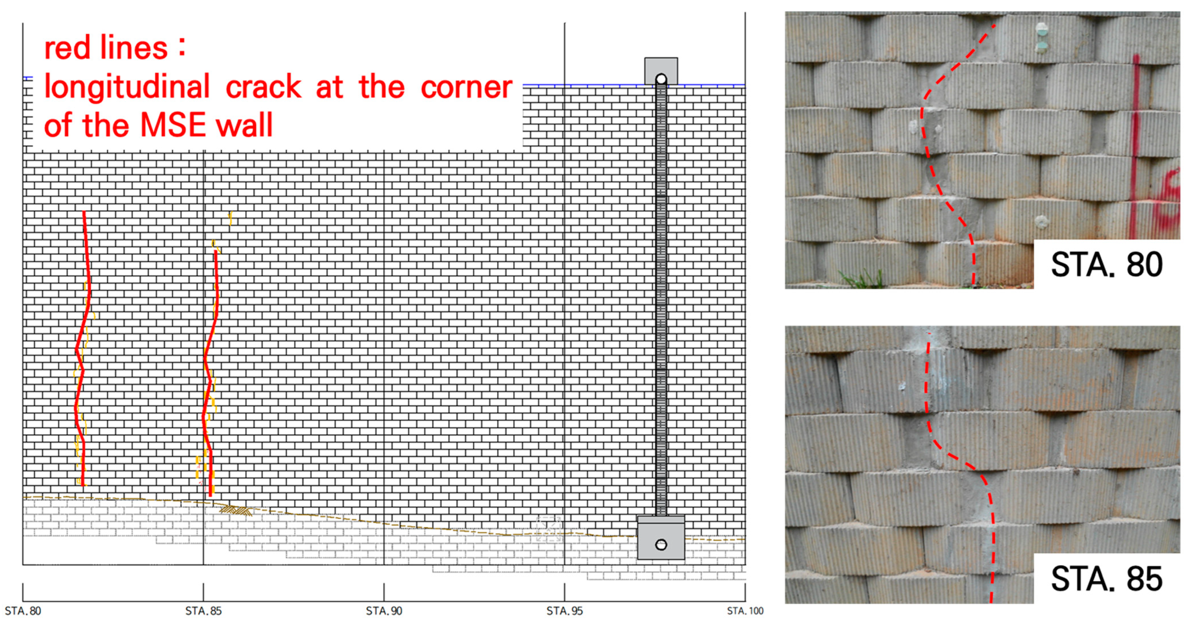
3.1. Evaluating the Cause of Cracks on the MSE Wall Facing at the Case Site

The results of the electrical resistivity survey were analyzed to evaluate the cause of the cracks in the wall facing of the MSE wall at the case site. Although electrical resistivity surveys are not very quantitative in terms of ground properties, they are useful in determining the overall subsurface conditions (soil type, presence of voids, groundwater conditions, etc.).

Figure 8 shows the results of the electrical resistivity survey of the MSE wall.

Figure 8a to Figure 8c show the results of the original ground exploration focused on the front of the MSE wall. There were no abnormal areas in ER-1-1 and ER-1-2 (Figure 8a). However, four abnormal areas were identified as a result of the ER-1-3 exploration. Based on the past construction history of the MSE wall, areas A and D were among the abnormal areas evaluated due to the drainage pipes in the original ground in front of the MSE wall. Moreover, area C was identified as being affected by a collector well, which is a reinforced concrete structure. Area B, which is the exploration result for the ground where the corner of the MSE wall is located, was analyzed to be an abnormal area caused by low ground stiffness since there was no history of underground construction structures. This means that it had a great influence on the occurrence of longitudinal cracks in the facing of the MSE wall. Area E, which can be seen in the exploration results of ER-1-4, was also identified as being affected by underground structures. Therefore, it was analyzed that the low ground stiffness of the original ground in the structurally vulnerable corner induced the displacement of the MSE wall due to subsidence, based on the exploration results of the original ground in the front of the MSE wall.

Figure 8d to Figure 8e show the exploration results of the reinforced earth mass in the MSE wall. It was found that there was no abnormal area in ER-2-1, but two abnormal areas were confirmed in ER-2-2 and ER-2-3. Areas F and G correspond to the corners of the MSE wall, and the abnormal areas are connected. In addition, these areas have similar longitudinal cross-section locations to area B. In other words, it was found that the problems (such as groundwater infiltration) in areas F and G, which extended to area B, caused the continuous deformation of the corner on the MSE wall.

Therefore, the risk area for the MSE wall of the case site was determined to be the corner based on the results of the electrical resistivity survey. In other words, this area was evaluated as requiring continuous monitoring. The longitudinal crack status of the corner is shown in Figure 9.

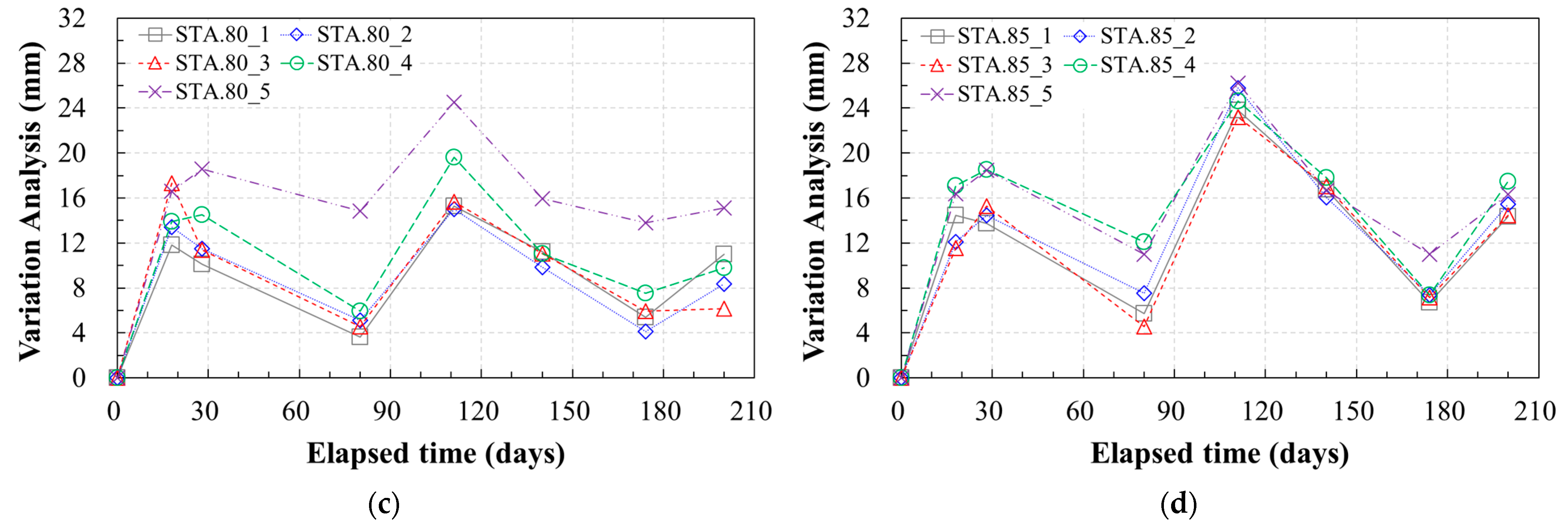
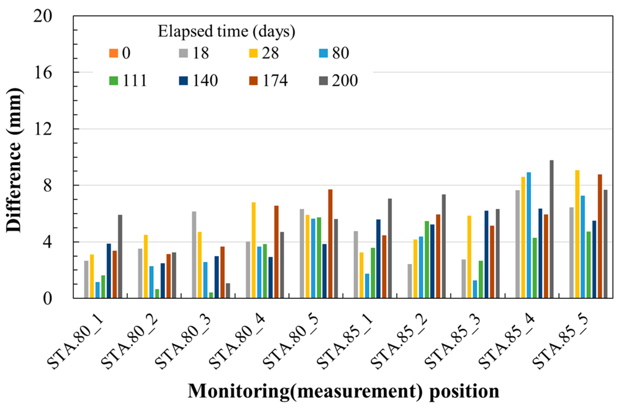
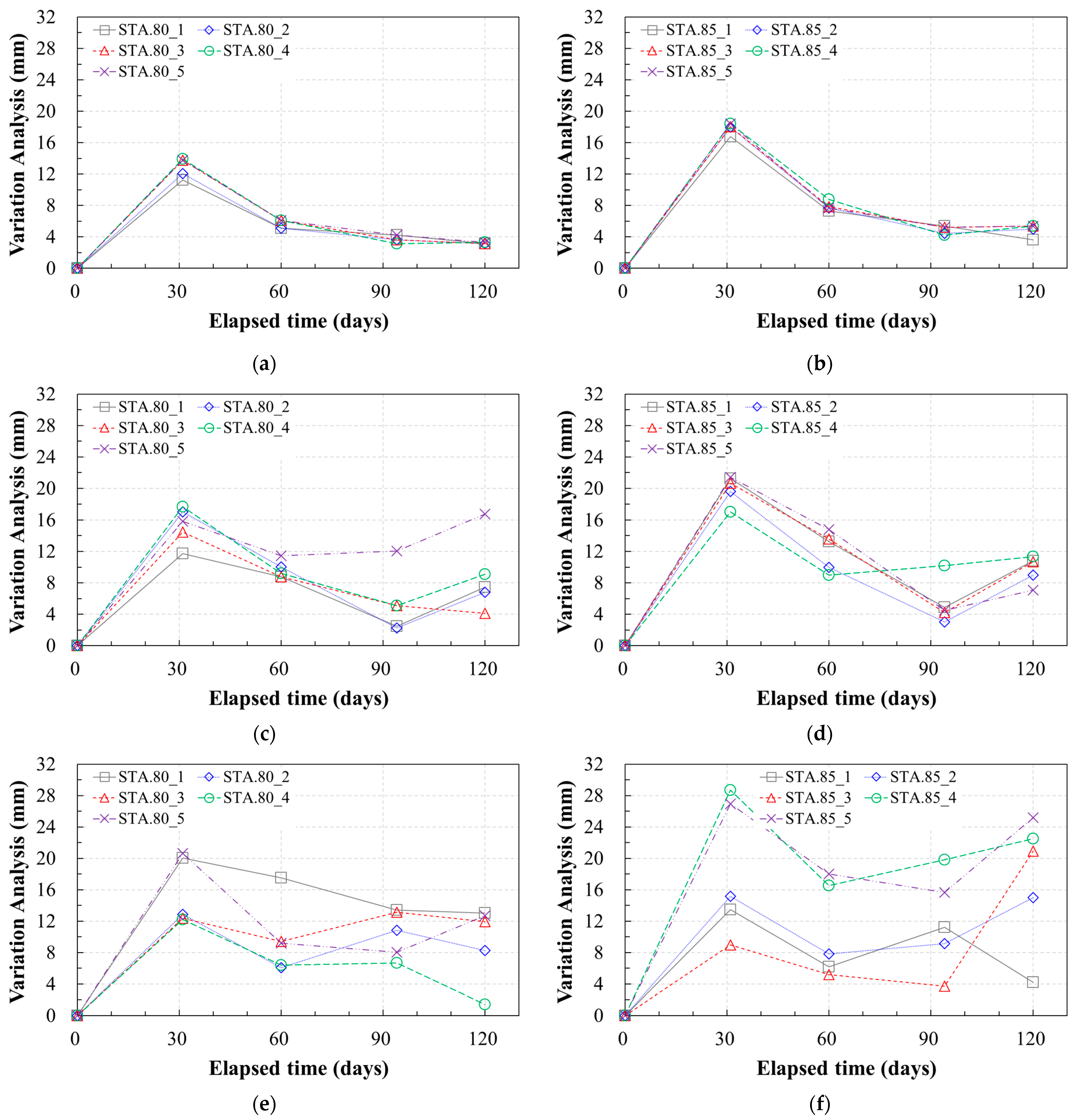
3.2. Monitoring Results

The traditional monitoring method (total station) and digital image photogrammetry (digital camera) were applied in the field for 7 months. In addition, cellphone-based digital image photogrammetry was applied in the field for 4 months. Therefore, this section describes the comparison results of traditional monitoring methods (total station) and digital image photogrammetry (digital camera and cellphone) using the results of field monitoring experiments.

Table 3. Monitoring results using traditional monitoring and digital image photogrammetry (7 months).

Elapsed Time (Days)	Measurement Point	Traditional Monitoring (Total Station)			Digital Photogrammetry (Digital Camera)			Variation Analysis of Traditional Monitoring (mm)	Variation Analysis of Digital Photogrammetry (mm)	Difference (mm)
		X	Y	Z	X′	Y′	Z′
0	80_1	1003.813	998.938	0.48	1003.81	998.942	0.481	0.000	0.000	0.000
	80_2	1003.833	998.864	2.026	1003.833	998.869	2.021	0.000	0.000	0.000
	80_3	1003.843	998.828	2.811	1003.843	998.836	2.813	0.000	0.000	0.000
	80_4	1003.863	998.755	4.017	1003.859	998.77	4.025	0.000	0.000	0.000
	80_5	1003.888	998.655	5.211	1003.883	998.689	5.221	0.000	0.000	0.000
	85_1	999.089	996.596	0.541	999.085	996.602	0.539	0.000	0.000	0.000
	85_2	999.1	996.557	1.754	999.094	996.56	1.752	0.000	0.000	0.000
	85_3	999.165	996.497	3.735	999.165	996.505	3.734	0.000	0.000	0.000
	85_4	999.21	996.479	4.567	999.203	996.489	4.563	0.000	0.000	0.000
	85_5	999.2	996.388	5.751	999.196	996.398	5.748	0.000	0.000	0.000
18	80_1	1003.821	998.94	0.484	1003.816	998.94	0.491	9.165	11.832	2.667
	80_2	1003.842	998.865	2.03	1003.841	998.865	2.031	9.899	13.416	3.517
	80_3	1003.853	998.828	2.816	1003.857	998.826	2.815	11.180	17.321	6.140
	80_4	1003.872	998.756	4.021	1003.867	998.759	4.022	9.899	13.928	4.029
	80_5	1003.897	998.655	5.216	1003.879	998.673	5.223	10.296	16.613	6.318
	85_1	999.098	996.593	0.539	999.097	996.594	0.54	9.695	14.457	4.761
	85_2	999.108	996.552	1.752	999.105	996.555	1.752	9.644	12.083	2.439
	85_3	999.173	996.494	3.733	999.171	996.496	3.73	8.775	11.533	2.758
	85_4	999.219	996.477	4.565	999.215	996.477	4.561	9.434	17.088	7.654
	85_5	999.209	996.385	5.748	999.208	996.388	5.753	9.950	16.401	6.451
28	80_1	1003.819	998.94	0.483	1003.82	998.941	0.482	7.000	10.100	3.100
	80_2	1003.839	998.866	2.029	1003.841	998.867	2.029	7.000	11.489	4.489
	80_3	1003.849	998.828	2.814	1003.852	998.829	2.813	6.708	11.402	4.694
	80_4	1003.87	998.756	4.02	1003.872	998.766	4.02	7.681	14.491	6.810
	80_5	1003.894	998.666	5.213	1003.895	998.678	5.212	12.689	18.601	5.912
	85_1	999.099	996.595	0.544	999.096	996.6	0.547	10.488	13.748	3.260
	85_2	999.109	996.553	1.757	999.108	996.557	1.754	10.296	14.457	4.161
	85_3	999.173	996.493	3.738	999.174	996.493	3.737	9.434	15.297	5.863
	85_4	999.219	996.476	4.57	999.217	996.477	4.565	9.950	18.547	8.597
	85_5	999.208	996.384	5.754	999.207	996.384	5.753	9.434	18.493	9.059
80	80_1	1003.815	998.939	0.479	1003.813	998.944	0.481	2.449	3.606	1.156
	80_2	1003.835	998.866	2.026	1003.832	998.869	2.026	2.828	5.099	2.271
	80_3	1003.845	998.828	2.811	1003.847	998.835	2.815	2.000	4.583	2.583
	80_4	1003.865	998.756	4.017	1003.858	998.765	4.022	2.236	5.916	3.680
	80_5	1003.89	998.664	5.211	1003.883	998.679	5.21	9.220	14.866	5.647
	85_1	999.093	996.596	0.541	999.089	996.601	0.543	4.000	5.745	1.745
	85_2	999.103	996.556	1.754	999.101	996.558	1.754	3.162	7.550	4.388
	85_3	999.168	996.496	3.736	999.166	996.501	3.736	3.317	4.583	1.266
	85_4	999.213	996.479	4.568	999.21	996.48	4.567	3.162	12.083	8.921
	85_5	999.203	996.386	5.752	999.202	996.392	5.755	3.742	11.000	7.258
111	80_1	1003.824	998.942	0.473	1003.824	998.948	0.482	13.638	15.264	1.626
	80_2	1003.844	998.870	2.019	1003.843	998.858	2.019	14.353	15.000	0.647
	80_3	1003.855	998.833	2.803	1003.854	998.831	2.803	15.264	15.684	0.420
	80_4	1003.876	998.759	4.009	1003.871	998.766	4.01	15.780	19.621	3.842
	80_5	1003.901	998.666	5.203	1003.898	998.678	5.205	18.815	24.536	5.721
	85_1	999.107	996.590	0.534	999.106	996.592	0.534	20.224	23.791	3.567
	85_2	999.118	996.549	1.747	999.117	996.55	1.746	20.322	25.788	5.465
	85_3	999.183	996.490	3.728	999.182	996.49	3.729	20.543	23.216	2.674
	85_4	999.226	996.468	4.561	999.222	996.475	4.556	20.322	24.617	4.295
	85_5	999.216	996.375	5.745	999.213	996.379	5.742	21.471	26.192	4.721
140	80_1	1003.82	998.940	0.479	1003.821	998.941	0.479	7.348	11.225	3.877
	80_2	1003.84	998.866	2.025	1003.842	998.869	2.025	7.348	9.849	2.500
	80_3	1003.851	998.828	2.810	1003.851	998.829	2.81	8.062	11.045	2.983
	80_4	1003.871	998.756	4.016	1003.867	998.763	4.022	8.124	11.045	2.921
	80_5	1003.896	998.664	5.210	1003.888	998.674	5.219	12.083	15.937	3.854
	85_1	999.1	996.594	0.541	999.101	996.597	0.539	11.180	16.763	5.583
	85_2	999.11	996.553	1.753	999.11	996.561	1.751	10.817	16.062	5.246
	85_3	999.175	996.493	3.734	999.176	996.492	3.734	10.817	17.029	6.213
	85_4	999.221	996.476	4.566	999.216	996.477	4.561	11.446	17.804	6.359
	85_5	999.21	996.383	5.751	999.207	996.387	5.742	11.180	16.673	5.493
174	80_1	1003.811	998.938	0.480	1003.814	998.945	0.479	2.000	5.385	3.385
	80_2	1003.832	998.864	2.026	1003.834	998.869	2.025	1.000	4.123	3.123
	80_3	1003.842	998.826	2.811	1003.848	998.835	2.81	2.236	5.916	3.680
	80_4	1003.862	998.755	4.017	1003.863	998.765	4.021	1.000	7.550	6.550
	80_5	1003.887	998.661	5.211	1003.892	998.679	5.218	6.083	13.784	7.701
	85_1	999.088	996.598	0.541	999.091	996.599	0.539	2.236	6.708	4.472
	85_2	999.099	996.558	1.754	999.101	996.558	1.751	1.414	7.348	5.934
	85_3	999.163	996.497	3.735	999.166	996.498	3.733	2.000	7.141	5.141
	85_4	999.209	996.480	4.567	999.202	996.482	4.561	1.414	7.348	5.934
	85_5	999.198	996.387	5.751	999.198	996.392	5.757	2.236	11.000	8.764
200	80_1	1003.818	998.939	0.480	1003.819	998.948	0.479	5.099	11.000	5.901
	80_2	1003.838	998.865	2.026	1003.838	998.872	2.027	5.099	8.367	3.268
	80_3	1003.848	998.827	2.811	1003.849	998.837	2.812	5.099	6.164	1.065
	80_4	1003.868	998.755	4.016	1003.867	998.766	4.021	5.099	9.798	4.699
	80_5	1003.893	998.663	5.210	1003.897	998.685	5.217	9.487	15.100	5.613
	85_1	999.096	996.594	0.541	999.096	996.593	0.541	7.280	14.353	7.073
	85_2	999.107	996.553	1.754	999.109	996.562	1.755	8.062	15.427	7.365
	85_3	999.172	996.493	3.734	999.173	996.493	3.735	8.124	14.457	6.333
	85_4	999.217	996.476	4.566	999.218	996.481	4.559	7.681	17.464	9.783
	85_5	999.207	996.383	5.750	999.203	996.385	5.755	8.660	16.340	7.680

shows the results of the field monitoring conducted for 7 months.

The values presented in the table have the following meanings.

The 3D coordinates of traditional monitoring and digital image photogrammetry represent the results measured using the total station and digital camera, respectively. The values in the columns of ‘Variation Analysis Of Traditional Monitoring’ and ‘Variation Analysis Of Digital Photogrammetry’ are the results obtained by converting each 3D coordinate into a displacement vector. Moreover, ‘Difference’ represents the difference between each displacement vector.

Based on the measurement results, the elapsed time–displacement relationship according to the position of the wall facing was plotted, as shown in Figure 10.

First, the total station measurements were analyzed. It was found that the displacement at STA.80 ranged from a minimum of 1 mm (STA.80_2, STA.80_4) to a maximum of 18.815 mm (STA.80_5). The change in displacement over time showed similar shapes for STA.80_1–STA.80_5, but the displacement at STA.80_5 was larger than that at the other points. The height of the measurement point STA.80_5 was 5.2 m from the bottom of the MSE wall, which was approximately 37% of the total height of the MSE wall (14.1 m). It is typical for the wall facing deformation of an MSE wall to have the largest deformation in the first one-third segment of the total height (approximately 33% of the total height). This implies that STA.80_5 had a larger deformation at the corner. The displacements at STA.85 were found to range from a minimum of 1.414 mm (STA.85_2, STA.85_4) to a maximum of 21.471 mm (STA.85_5). The evolution of the displacement over time and quantitative displacement values were found to be almost similar for all points, and the displacement at STA.85 was slightly larger than that at STA.80 for less than one-third of the total height. This agreed with the analysis of the cause of the displacement at STA.80.

The digital image photogrammetry results, obtained using a digital camera, were analyzed. The displacement at the corner of STA.80 was found to be a minimum of 3.606 mm (STA.80_1) and a maximum of 24.536 mm (STA.80_5). The temporal changes in the displacement were similar for STA.80_1 to STA.80_5. However, the quantitative displacement values were somewhat larger than the displacement values for the total station, and some were irregular. In particular, the displacements at STA.80_4 and STA.80_5 were found to be large. The displacements at the corner of STA.85 were found to range from a minimum of 4.583 mm (STA.85_3) to a maximum of 26.192 mm (STA.85_5). This was similar to the observation for STA.80, and it was much larger than the displacement value obtained from the traditional monitoring method (total station).

The measurement and monitoring results of the traditional monitoring method and digital camera-based digital image photogrammetry revealed significant wall facing displacements at 18, 28, and 111 days. These were attributed to a large amount of rainfall that occurred just before the elapsed time due to the seasonal characteristics of South Korea; the rainfall penetrated the anomalous area found in the electrical resistivity survey’s results, causing the wall facing’s displacement.

Based on the measurement and monitoring results evaluated above, the difference between the measurement results of the traditional monitoring method and digital camera-based digital image photogrammetry was calculated. Figure 11 shows the measurement position error as a function of the elapsed time. Due to the high reliability of the traditional monitoring method, which is the total station, the displacement error was defined as the difference between the displacement values obtained with the traditional monitoring method and digital camera-based digital image photogrammetry.

For STA.80, the two highest error levels occurred at 80 days and 174 days from the initial measurement date. STA.85 showed similar results. The largest errors occurred at positions STA.80_4–STA.80_5 and STA.85_4–STA.85_5, which means that the error was larger when the displacement was relatively large.

Table 4. Monitoring results using traditional monitoring and digital image photogrammetry (4 months).

Elapsed Time (Days)	Measurement Point	Variation Analysis of Traditional Monitoring (Total Station) (mm)	Variation Analysis of Digital Image Photogrammetry (Digital Camera) (mm)	Variation Analysis of Digital Image Photogrammetry (Cellphone Camera) (mm)	Difference between Traditional Monitoring and Digital Image Photogrammetry (Digital Camera) (mm)	Difference between Traditional Monitoring and Digital Image Photogrammetry (Cellphone Camera) (mm)
0	80_1	0.000	0.000	0.000	0.000	0.000
	80_2	0.000	0.000	0.000	0.000	0.000
	80_3	0.000	0.000	0.000	0.000	0.000
	80_4	0.000	0.000	0.000	0.000	0.000
	80_5	0.000	0.000	0.000	0.000	0.000
	85_1	0.000	0.000	0.000	0.000	0.000
	85_2	0.000	0.000	0.000	0.000	0.000
	85_3	0.000	0.000	0.000	0.000	0.000
	85_4	0.000	0.000	0.000	0.000	0.000
	85_5	0.000	0.000	0.000	0.000	0.000
31	80_1	11.225	11.747	20.025	0.522	8.800
	80_2	12.083	17.059	12.884	4.976	0.801
	80_3	13.748	14.457	12.369	0.709	1.378
	80_4	13.928	17.720	12.207	3.792	1.722
	80_5	13.748	15.843	20.664	2.095	6.916
	85_1	16.763	21.237	13.454	4.474	3.309
	85_2	17.972	19.596	15.166	1.624	2.806
	85_3	18.028	20.640	9.000	2.612	9.028
	85_4	18.412	17.029	28.705	1.383	10.293
	85_5	18.412	21.424	26.926	3.012	8.514
60	80_1	5.099	8.775	17.521	3.676	12.422
	80_2	5.099	10.050	6.083	4.951	0.984
	80_3	6.083	8.775	9.434	2.692	3.351
	80_4	6.083	9.220	6.403	3.137	0.320
	80_5	6.083	11.446	9.220	5.363	3.137
	85_1	7.280	13.266	6.164	5.986	1.116
	85_2	7.681	9.950	7.810	2.269	0.129
	85_3	7.874	13.601	5.196	5.727	2.678
	85_4	8.775	9.000	16.523	0.225	7.748
	85_5	7.681	14.799	18.000	7.118	10.319
94	80_1	4.243	2.449	13.416	1.793	9.174
	80_2	3.606	2.236	10.863	1.369	7.257
	80_3	3.606	5.099	13.153	1.493	9.547
	80_4	3.162	5.099	6.708	1.937	3.546
	80_5	4.243	12.042	8.062	7.799	3.820
	85_1	5.385	4.899	11.225	0.486	5.840
	85_2	4.472	3.000	9.165	1.472	4.693
	85_3	5.196	4.243	3.742	0.954	1.454
	85_4	4.243	10.198	19.824	5.955	15.582
	85_5	5.196	4.472	15.652	0.724	10.456
120	80_1	3.162	7.483	13.038	4.321	9.876
	80_2	3.162	6.782	8.246	3.620	5.084
	80_3	3.162	4.123	11.916	0.961	8.754
	80_4	3.317	9.110	1.414	5.794	1.902
	80_5	3.317	16.763	12.689	13.446	9.372
	85_1	3.606	10.817	4.243	7.211	0.637
	85_2	5.000	9.000	15.000	4.000	10.000
	85_3	5.385	10.677	20.905	5.292	15.519
	85_4	5.385	11.358	22.494	5.973	17.109
	85_5	5.385	7.071	25.199	1.686	19.814

shows the results of the comparison conducted for 4 months using traditional monitoring and digital image photogrammetry methods (using digital cameras and cellphone cameras). The 3D coordinate data of the monitoring results using three types of devices are very large. Therefore, the values expressed in Table 4 are the displacement vectors calculated using 3D coordinates and the vector difference between the traditional monitoring method and digital image photogrammetry (digital camera and cellphone camera).

Figure 12 shows a plot of the elapsed time and the displacement of each measurement point obtained using traditional monitoring and digital image photogrammetry methods.

Figure 12a,b show the results of the traditional monitoring method. Despite the differences between the displacement values of the neighboring STA.80 and STA.85, a similar trend was observed in the temporal changes in the displacement. The minimum and maximum displacements at STA.80 and STA.85 were 3.162–13.928 mm and 4.472–18.412 mm, respectively.

As shown in Figure 12c,d, the measurement results of the digital camera-based digital image photogrammetry showed that the minimum and maximum displacements of STA.80 were 2.236 mm and 17.747 mm, and the minimum and maximum displacements of STA.85 were 3 mm and 21.424 mm. In particular, the displacement values at 120 days were found to be relatively much larger than those obtained via traditional monitoring.

Figure 12e,f show the digital image photogrammetry measurements obtained using the cellphone camera. Regardless of the monitoring area, the displacement occurrence trend was similar to that of traditional monitoring and the digital camera with respect to the initial elapsed time, but the measurements were very irregular thereafter.

Figure 13 shows the evaluation results of the digital image photogrammetry error based on each commercial imaging device against the traditional monitoring method using the measurement results.

The results of digital camera-based digital image photogrammetry show that the measurement values for low-level displacements were less different from those of the traditional monitoring method. However, the errors between the two methods were shown to be large when displacements were large. In addition, the measurement errors of cellphone camera-based digital image photogrammetry were evaluated to be at a level that was not meaningful for analysis compared to the measurement results of other methods; thus, they were excluded from discussion in this study.

3.3. Discussion of Applicability of Digital Image Photogrammetry

This section discusses the applicability of digital image photogrammetry (using digital cameras and cellphone cameras) for studying the displacement measurement of MSE walls in restricted and controlled areas. The discussion on applicability is presented by analyzing the error rate. The error rate is defined as the percentage of each digital image photogrammetry error with respect to the value assuming the reliability of the measurement results of the traditional monitoring method to be 1.

First, the error rate was evaluated through field experiment results conducted for about 7 months using the traditional monitoring method and digital camera-based digital image photogrammetry. The error rate of the digital camera was found to be the largest when the elapsed time was 174 days. In particular, as shown in Figure 14a, the maximum error rate was 655% in STA.80_4, and the error rates of STA.85_4 and STA.85_5 were 433% and 516%, respectively.

Through a field experiment conducted for 4 months, the digital image photogrammetry error rate using a digital camera and a cellphone camera was evaluated and compared to the traditional monitoring method. As shown in Figure 14b, the error rate of the digital camera was the largest at 405% in STA.80_5, when the elapsed time was 120 days. The error of the digital camera occurred at a specific elapsed time and location, and it showed a similar error occurrence trend to the results of the experiment conducted for 7 months. Figure 14c shows the maximum error rate of the cellphone camera, and the maximum error rate was 367%, which was similar to that of the digital camera. However, the error rate of the cellphone camera showed a very irregular error occurrence trend regardless of the experimental period and location.

If the error rate trend is similar, it is easy to identify the error occurrence variable and reduce it. However, the cause of the error is very complicated if judging the error trend is difficult, such as the error trend of the cellphone camera. In this study, the measurement error of the cellphone camera was analyzed as a result of the combined effects of low pixels and image distortion on the location’s information. Therefore, it was found to be very unsuitable for evaluating the applicability of MSE wall displacement monitoring using cellphone camera-based digital image photogrammetry. In other words, it was evaluated that optical research is necessary to solve this.

4. Conclusions

This study experimentally evaluated the applicability of digital image photogrammetry in South Korea for the rapid measurement of MSE wall deformation in restricted-access and controlled areas. The results are summarized as follows.

• The cause of the facing crack of the MSE wall in this research’s case study site was evaluated based on the results of the electrical resistivity survey. The evaluation results confirmed that an abnormal area occurred in the corner of the structurally vulnerable MSE wall due to the groundwater infiltration of the original ground and reinforced earth mass. In other words, it was observed that it caused the facing crack and deformation of the MSE wall.
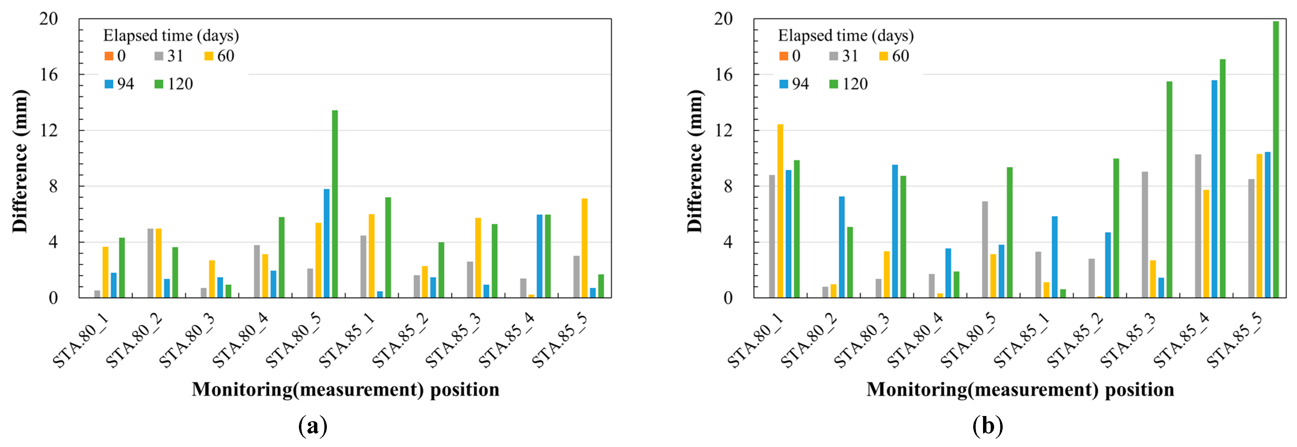
• In order to evaluate the applicability of digital image photogrammetry in restricted-access and controlled areas, the displacement of the MSE wall was monitored using the traditional monitoring method and digital image photogrammetry. The monitoring results showed that the displacement values showed similar elapsed time trends for both methods, but digital image photogrammetry results exhibited larger displacements than the traditional monitoring results. Nevertheless, the error of the digital camera applied for digital image photogrammetry was lower than that of the cellphone camera.
• In order to evaluate the accuracy of digital image photogrammetry, the error rate was analyzed. The results showed that the error at a specific location was similar between the digital camera and the cellphone camera. However, it was found that digital image photogrammetry using a digital camera with a consistent error occurrence tendency is highly applicable to rapid structural deformation monitoring in restricted-access and controlled areas.
• It was found that research on the effect of the camera’s pixels on the error was necessary in order to improve the accuracy and error resolution of digital image photogrammetry using a digital camera. In addition, the effect of the aligned image on the accuracy of the measurement coordinates in the 3D transformation of the 2D image acquired from the digital camera must be studied. It was also evaluated that the position of the digital camera may have contributed to the error rate of the measurement results. Therefore, research should continue to evaluate the limitations of the image acquisition distance and angle of the digital camera.

References

1. FHWA. Design of Mechanically Stabilized Earth Walls and Reinforced Soil Slopes-Volume I; FHWA-NHI-10-024; U.S. Department of Transportation: Washington, DC, USA, 2009.
2. Passe, P.D. Mechanically Stabilized Earth Wall Inspector’s Handbook; State of Florida, Department of Transportation: Tallahassee, FL, USA, 2000.
3. Yoo, C.; Jung, H.Y. Case History of Geosynthetic Reinforced Segmental Retaining Wall Failure. J. Geotech. Geoenviron. Eng. 2006, 132, 1538–1548. [Google Scholar] [CrossRef]
4. Won, M.S.; Kim, Y.S. Internal deformation behavior of geosynthetic-reinforced soil walls. Geotext. Geomembr. 2007, 25, 10–22. [Google Scholar] [CrossRef]
5. Bergado, D.T.; Teerawattanasuk, C. 2D and 3D numerical simulations of reinforced embankments on soft ground. Geotext. Geomembr. 2008, 26, 39–55. [Google Scholar] [CrossRef]
6. Chen, R.H.; Chiu, Y.M. Model tests of geocell retaining structures. Geotext. Geomembr. 2008, 26, 56–57. [Google Scholar] [CrossRef]
7. Li, A.L.; Rowe, R.K. Effects of viscous behavior of geosynthetic reinforcement and foundation soils on embankment performance. Geotext. Geomembr. 2008, 26, 317–334. [Google Scholar]
8. Rowe, R.K.; Taechakumthorn, C. Combined effect of PVDs and reinforcement on embankments over rate-sensitive soils. Geotext. Geomembr. 2008, 26, 239–249. [Google Scholar] [CrossRef]
9. Tatsuoka, F.; Hirakawa, D.; Nojiri, M.; Aizawa, H.; Nishikiori, H.; Soma, R.; Tateyama, M.; Watanabe, K. A new type of integral bridge comprising geosynthetic-reinforced soil walls. Geosynth. Int. 2009, 16, 301–326. [Google Scholar] [CrossRef]
10. Oskouie, P.; Becerik-Gerber, B.; Soibelman, L. Automated measurement of highway retaining wall displacements using terrestrial laser scanners. Autom. Constr. 2016, 65, 86–101. [Google Scholar] [CrossRef]
11. Rearick, A.; Khan, A. MSE Wall Design and Construction Policy Updates; State of Indiana, Department of Transportation: Indianapolis, IN, USA, 2017.
12. Al-Rawabdeh, A.; Aldosari, M.; Bullock, D.; Habib, A. Mobile LiDAR for Scalable Monitoring of Mechanically Stabilized Earth Walls with Smooth Panels. Appl. Sci. 2020, 10, 4480. [Google Scholar] [CrossRef]
13. Aldosari, M.; Al-Rawabdeh, A.; Bullock, D.; Habib, A. A Mobile LiDAR for Monitoring Mechanically Stabilized Earth Walls with Textured Precast Concrete Panels. Remote Sens. 2020, 12, 306. [Google Scholar] [CrossRef]
14. Budhu, M. Soil Mechanics & Foundations; John Wiley & Sons, Inc.: Hoboken, NJ, USA, 2000. [Google Scholar]
15. Bernhardt, K.L.S.; Loehr, J.E.; Huaco, D. Asset Management Framework for Geotechnical Infrastructure. J. Infrastruct. Syst. 2003, 9, 107–116. [Google Scholar] [CrossRef]
16. Giresini, L.; Puppio, M.L.; Taddei, F. Experimental pull-out tests and design indications for strength anchors installed in masonry walls. Mater. Struct. 2020, 53, 103. [Google Scholar] [CrossRef]
17. Palmeira, E.M. Soil-geosynthetic interation: Modelling and analysis. Geotext. Geomembr. 2009, 27, 368–390. [Google Scholar] [CrossRef]
18. ASTM D 6706-01; Standard Test Method for Measuring Geosynthetic Pullout Resistance in Soil. ASTM Book of Standards. ASTM International: Philadelphia, PA, USA, 2003; Volume 4, p. 13.
19. Hannah, M.J. A system for digital stereo image matching. Photogrammatic Eng. Remote Sens. 1989, 55, 1765–1770. [Google Scholar]
20. El-Hakim, S.F.; Wong, K.W. Working group V/1: Digital and real-time close-range photogrammetry. In Proceedings of the SPIE Proceedings, Close-Range Photogrammetry Meets Machine Vision, Bellingham, WA, USA, 3–7 September 1990. [Google Scholar]
21. Fraser, C.S. A resume of some industrial applications of photogrammetry. ISPRS J. Photogramm. Remote Sens. 1993, 48, 12–23. [Google Scholar] [CrossRef]
22. Fraser, C.S. Full Automation of Sensor Calibration, Exterior Orientation and Triangulation in Industrial Vision Metrology. In Proceedings of the International Workshop on Image Analysis and Information Fusion, Adelaide, Australia, 6–7 November 1997; pp. 13–24. [Google Scholar]
23. Oats, R.; Escobar-Wolf, R.; Oommen, T. A Novel Application of Photogrammetry for Retaining Wall Assessment. Infrastructures 2017, 2, 10. [Google Scholar] [CrossRef]
24. Anderson, S.A.; Rivers, B.S. Capturing the Impacts of Geotechnical Features on Transportation System Performance. In Proceedings of the Geo-Congress, San Diego, CA, USA, 28 March 2013; pp. 1633–1642. [Google Scholar]
25. Butler, C.J.; Gabr, M.A.; Rasdorf, W.; Findley, D.J.; Chang, J.C.; Hammit, B.E. RetainingWall Field Condition Inspection, Rating Analysis, and Condition Assessment. J. Perform. Constr. Facil. 2015, 30, 04015039. [Google Scholar] [CrossRef]
26. Brutus, O.; Tauber, G. Guide to Asset Management of Earth Retaining STRUCTURES; US Department of Transportation, Federal Highway Administration, Office of Asset Management: Washington, DC, USA, 2009.
27. Han, J.; Hong, K.; Kim, S. Application of a Photogrammetric System for Monitoring Civil Engineering Structures; InTech.: Rijeka, Croatia, 2012. [Google Scholar]
28. Wyllie, D.; Mah, C. Rock Slope Engineering Civil and Mining, 4th ed.; Spon Press: New York, NY, USA, 2004. [Google Scholar]
29. Scaioni, M.; Alba, M.; Roncoroni, F.; Giussani, A. Monitoring of a SFRC retaining structure during placement. Eur. J. Environ. Civ. Eng. 2010, 14, 467–493. [Google Scholar] [CrossRef]
30. Wang, G.; Philips, D.; Joyce, J.; Rivera, F. The integration of TLS and continuous GPS to study landslide deformation: A case study in Puerto Rico. J. Geod. Sci. 2011, 1, 25–34. [Google Scholar] [CrossRef]
31. Vaghefi, K.; Oats, R.; Harris, D.; Ahlborn, T.; Brooks, C.; Endsley, K.; Roussi, C.; Shuchman, R.; Burns, J.; Dobson, R. Evaluation of Commercially Available Remote Sensors for Highway Bridge Condition Assessment. J. Bridge Eng. 2012, 17, 886–895. [Google Scholar] [CrossRef]
32. Escobar-Wolf, R.; Oommen, T.; Brooks, C.; Dobson, R.; Ahlborn, T. Unmanned Aerial Vehicle (UAV)-based Assessment of Concrete Bridge Deck Delamination Using Thermal and Visible Camera Sensors: A Preliminary Analysis. Res. Nondestr. Eval. 2017, 29, 183–198. [Google Scholar] [CrossRef]
33. Jiang, R.; Jauregui, D.V.; White, K.R. Close-Range Photogrammetry Applications in Bridge Measurement: Literature Review. Measurement 2008, 41, 823–834. [Google Scholar] [CrossRef]
34. Gong, J.; Zhou, H.; Gordon, C.; Jalayer, M. Mobile Terrestrial Laser Scanning for Highway Inventory Data Collection. Comp. Civ. Eng. 2012, 2012, 545–552. [Google Scholar] [CrossRef]
35. Olsen, M.J.; Butcher, S.; Silvia, E.P. Real-Time Change and Damage Detection of Landslides and Other Earth Movements Threatening Public Infrastructure; Transportation Research and Education Center (TREC): Portland, OR, USA, 2012; OTREC-RR-11-23. [Google Scholar]
36. Xiao, R.; He, X. GPS and InSAR Time Series Analysis: Deformation Monitoring Application in a Hydraulic Engineering Resettlement Zone, Southwest China. Math. Prob. Eng. 2013, 2013, 601209. [Google Scholar] [CrossRef]
37. Casagli, N.; Cigna, F.; Bianchini, S.; Hölbling, D.; Füreder, P.; Righini, G.; Vlcko, J. Landslide mapping and monitoring by using radar and optical remote sensing: Examples from the EC-FP7 project SAFER. Remote Sens. Appl. Soc. Environ. 2016, 4, 92–108. [Google Scholar] [CrossRef]
38. Laefer, D.; Lennon, D. Viability assessment of terrestrial LiDAR for retaining wall monitoring. In Proceedings of the American Society of Civil Engineers, GeoCongress 2008: Geosustainability and Geohazard Mitigation, New Orleans, LA, USA, 9–12 March 2008; pp. 247–254. [Google Scholar]
39. Fischler, M.A.; Bolles, R.C. Random sample consensus: A paradigm for model fitting with applications to image analysis and automated cartography. Commun. ACM 1981, 24, 381–395. [Google Scholar] [CrossRef]
40. Lin, Y.J.; Habib, A.; Bullock, D.; Prezzi, M. Application of High-Resolution Terrestrial Laser Scanning to Monitor the Performance of Mechanically Stabilized EarthWalls with Precast Concrete Panels. J. Perform. Constr. Facil. 2019, 33, 04019054. [Google Scholar] [CrossRef]
41. Lienhart, W.; Monsberger, C.; Kalenjuk, S.; Woschitz, H. High Resolution Monitoring of Retaining Walls with Distributed Fibre Optic Sensors and Mobile Mapping Systems. In Proceedings of the 7th Asia-Pacific Workshop on Structural Health Monitoring, Hong Kong, China, 12–15 November 2018. [Google Scholar]
42. Kraus, K. Photogrammetry: Geometry from Images and Laser Scans; Walter de Gruyter: Berlin, Germany, 2007; ISBN 978-3-11-019007-6. [Google Scholar]
43. Golparvar-Fard, M.; Balali, V.; de la Garza, J.M. Segmentation and recognition of highway assets using image-based 3D point clouds and semantic Texton forests. J. Comp. Civ. Eng. 2012, 29, 04014023. [Google Scholar] [CrossRef]
44. Cleveland, L.; Wartman, J. Principles and Applications of Digital Photogrammetry for Geotechnical Engineering. Proc. Site Geomat. Charact. 2006, 16, 128–135. [Google Scholar]
45. Westoby, M.J.; Brasington, J.; Glasser, N.F.; Hambrey, M.J.; Reynolds, J.M. Structure-for-Motion’ photogrammetry: A low-cost, effective tool for geoscience applications. Geomorphology 2012, 179, 300–314. [Google Scholar] [CrossRef]
46. Wolf, P.R.; Dewitt, B.A. Elements of Photogrammetry: With Applications in GIS, 3rd ed.; McGraw-Hill Co. Inc.: New York, NY, USA, 2000. [Google Scholar]
Figure 1. Field floor plan of MSE wall: (a) MSE wall construction plan view; (b) representative cross-section of MSE wall.
Applsci 14 05295 g001
Figure 2. Geotechnical survey locations.
Applsci 14 05295 g002
Figure 3. Electrical resistivity survey instrument specifications.
Applsci 14 05295 g003
Figure 4. Electrical resistivity survey location plan view at the MSE wall site.
Applsci 14 05295 g004
Figure 5. Comparison of monitoring methods for MSE walls: (a) traditional monitoring procedure; (b) digital image photogrammetry procedure based on commercial imaging devices.
Applsci 14 05295 g005
Figure 6. Displacement measurement locations on the MSE wall: (a) STA. 80; (b) STA. 85.
Applsci 14 05295 g006
Figure 7. Field experiments with the traditional monitoring method (total station) and digital image photogrammetry (commercial imaging devices, digital camera, and cellphone camera).
Applsci 14 05295 g007
Figure 8. Electrical resistivity survey results: (a) ER-1-1 and ER-1-2; (b) ER-1-3; (c) ER-1-4; (d) ER-2-1; (e) ER-2-2 and ER-2-3.
Applsci 14 05295 g008aApplsci 14 05295 g008b
Figure 9. Corner crack status of the MSE wall.
Applsci 14 05295 g009
Figure 10. Elapsed time–displacement relationship depending on the position of the wall facing (monitoring for 7 months): (a) total station value [STA.80]; (b) total station value [STA.85]; (c) digital camera value [STA.80]; (d) digital camera value [STA.85].
Applsci 14 05295 g010aApplsci 14 05295 g010b
Figure 11. Difference between displacements obtained using the traditional monitoring method and digital camera-based digital image photogrammetry.
Applsci 14 05295 g011
Figure 12. Elapsed time–displacement relationship depending on the position of the wall facing (monitoring for 4 months): (a) total station value [STA.80]; (b) total station value [STA.85]; (c) digital camera value [STA.80]; (d) digital camera value [STA.85]; (e) cellphone camera value [STA.80]; (f) cellphone camera value [STA.85].
Applsci 14 05295 g012
Figure 13. Difference in displacement between total station and digital camera and cellphone camera results: (a) total station–digital camera; (b) total station–cellphone camera.
Applsci 14 05295 g013
Figure 14. Error rate analysis: (a) traditional monitoring method vs. digital image photogrammetry (digital camera), 7-month monitoring period; (b) traditional monitoring method vs. digital image photogrammetry (digital camera), 4-month monitoring period; (c) traditional monitoring method vs. digital image photogrammetry (cellphone camera), 7-month monitoring period.
Applsci 14 05295 g014