Research on Fault Prediction Method for Electric Multiple Unit Gearbox Based on Gated Recurrent Unit–Hidden Markov Model

Abstract

Due to the limited availability of fault samples and the expensive nature of marking fault samples in Electric Multiple Unit (EMU) gearbox monitoring data, a study was conducted to simulate the degradation process of key components in the CRH5 gearbox using rigid–flexible coupling dynamics. Vibration acceleration data from the simulation were utilized to create a six-dimensional hybrid feature domain representing the degradation process. By leveraging the capabilities of the Hidden Markov Model (HMM) for handling hidden transitive probabilities in temporal data and Gated Recurrent Unit (GRU) for addressing long-distance and high-dependence temporal data, a GRU-HMM fault prediction model was developed. This model was validated using monitoring data and the six-dimensional hybrid feature domain from the CRH5 gearbox and compared against actual maintenance records. The findings indicated that the GRU-HMM fault prediction model can effectively recognize the degradation patterns of multiple components, offering higher accuracy in fault prediction compared to traditional models. These research outcomes are expected to optimize EMU maintenance schedules based on usage conditions, enhance EMU utilization rates, and reduce operational and maintenance costs, thereby providing valuable theoretical support.

1. Introduction

As an important part of the traction transmission system, the gearbox affects the safety and stability of the Electric Multiple Unit (EMU). The components within the gearbox are subject to diverse loads, resulting in different types of malfunctions. Hence, analyzing operational data from the gearbox and anticipating potential failures are essential for ensuring the operational safety of the EMU.

The traditional method of mechanical system fault diagnosis involves using fault samples with label information to construct a fault diagnosis model for rotating machinery gearboxes, decomposing the complex vibration signals into modal functions, and analyzing the single modes so as to reflect the local characteristics of non-smooth signals [1,2,3]. This method of modal decomposition is characterized by the instantaneous identification of features but requires a large amount of data to produce effective results [4,5,6]. With the development of artificial intelligence, deep learning methods have become the main research direction of current fault diagnosis due to the advantages of efficient and powerful feature extraction, and methods of deep learning mainly include support vector machines and neural network algorithms [7,8,9,10]. The support vector machine still remains effective when the data dimension is larger than the number of samples, and it excels at solving nonlinear problems. However, SVM is sensitive to noisy data, not applicable to multi-class classification problems, and cannot directly provide probability estimates [11,12,13,14]. Neural networks have self-learning functions, can extract useful information from data through learning, have the ability to find optimization solutions at high speed, and can quickly find solutions when dealing with complex problems. However, the training and development of neural networks usually require a large amount of computational resources, which may increase the cost [15,16,17,18,19,20].

In rail train fault diagnosis research, due to the difficulty of obtaining fault characteristics from actual operation monitoring data, most scholars use accelerated life experiments or dynamics simulation to obtain the fault characteristics of key components and use deep learning algorithms to categorize and predict the fault characteristics [21,22]. Generally, the frequency response function between acceleration signals is analyzed as a fault indicator by establishing a dynamic model of the train or a specific component and analyzing the impact of radial and axial vibration under different fault conditions [23,24]. Then, using an RNN or CNN, normal and fault conditions are classified and recognized [25,26,27,28]. However, in fault identification for EMU gearboxes, the complexity of the vibration response signal components makes it difficult to extract the characteristic signals. Additionally, the high cost of marking the fault samples through accelerated life experiments further complicates the process. How to carry out accurate fault prediction and diagnosis of key components of rolling stock through dynamics simulation and other cost-effective methods is the current problem of fault prediction that needs to be solved in the field of rail transportation.

In summary, to solve the fault prediction problem of the scarcity of fault samples for the EMU gearbox, this paper establishes a rigid–flexible coupling dynamics model of the gearbox, taking into account the special characteristics of the CRH5 in the structure of the gearbox and the completeness of the collected data. The focus is on studying the universal joints, driving gear, and driven gears, which are the most frequent faults of the gearbox system of CRH5, as the objects of the study. Based on the rigid–flexible coupling dynamics model of the gearbox, the dynamics simulation of the whole life cycle degradation process of the key components is carried out. Using the vibration and acceleration data of the degradation process, a hybrid feature domain for the degradation of key components of the gearbox is constructed. This approach addresses the problem of fault feature extraction under the condition of scarcity of fault samples of the gearbox of the moving train. A fault prediction model of the EMU gearbox based on GRU-HMM is proposed, which overcomes the limitation of the traditional HMM regarding the input sequence length. This model improves the fault prediction performance and improves the comprehensive identification accuracy of the GRU-HMM fault prediction model by 15% compared to traditional HMM and SVM fault prediction models. The research results improve the reliability of gearbox failure prediction for EMU, improve the efficiency of EMU utilization, reduce the cost of utilization and maintenance, and provide theoretical support for the transformation of the maintenance mode into state repair. At the same time, it can also guarantee safe operation, which has very important practical application value.

2. GRU-HMM Fault Prediction Model

2.1. Demand Analysis of GRU-HMM Fault Prediction Model

The transmission structure of the CRH5 is traction motor-universal shaft-gearbox, and vibration acceleration and temperature data are collected simultaneously during operation. The monitoring data capacity of one primary repair cycle is about 200,000 items, and the data show time series characteristics, which are typical large-capacity and long-range time series data. The Hidden Markov Model (HMM) is capable of modeling probability distributions of time-series data, and the hidden state setting is well suited for multi-component fault prediction studies. However, HMM has a limitation on the length of the input sequence, has weak performance in dealing with dependencies over long distances, and is prone to problems such as gradient vanishing and gradient explosion. Therefore, the fusion of a Gated Recurrent Unit (GRU) with the HMM can solve the shortcomings in the performance of the HMM and provide better access to the dependencies of long sequence data, and its gating mechanism can also effectively solve the problems of gradient vanishing and gradient explosion, which can effectively improve the accuracy of the fault prediction model.

2.2. Hidden Markov Fault Prediction Model

The HMM fault prediction model uses monitoring data and sets the initial model parameters to maximize the conditional probability of the observed sequence using the Baum–Welch algorithm [29,30]. The HMM fault prediction model can be formulated as follows: $\lambda =(\pi ,A,B)$. It contains two state sets and three probability sets. On-site research and literature analysis indicates that the most common reason for failure of the CRH5 gearbox is universal joint and gear wear. Considering this characteristic, the HMM fault prediction model is modeled as follows:

• The hidden state Q is defined as Q = {normal state, universal joint degradation, driving gear degradation, driven gear degradation}, representing the hidden fault states of the CRH5 gearbox; here, the hidden state N = 4.
• Observable state O, denoted as O = {o₁, o₂, …, o_N}, where o_i ϵ (v₁, v₂, …, v_t), is a dataset for monitoring the operating status of the CRH5. Here, observable state v_t is a feature vector capturing the data characteristics of the train running up to the moment t under the four hidden states mentioned above.
• Initial vector π,

  $$\prod =({\pi }_1,{\pi }_2,{\pi }_3,\dots ,{\pi }_N)=\frac{C(i)}{{\displaystyle \sum _{S=1}^{N}C(s)}},{\pi }_i=P(q_i=s_i),1\le i\le N$$

  (1)

  indicates the probability that the degraded state of the component occurs at the initial time, where C(i) is the probability that the initial state is q_i.
• State transition matrix $A={\left\{a_{ij}\right\}}_{N\ast N}$,

  $$a_{ij}=P(q_{i+1}=s_j\left|q_i\right.=s_i)=\frac{A_{ij}}{{\displaystyle \sum _{S=1}^N{A}_{is}}},1\le i,j\le N$$

  (2)

  denotes the transfer probability of the gearbox component from state s_i to state s_j.
• Confusion matrix B,

  $$B={\left\{b_j(v_i)\right\}}_{N\ast M},b_j(v_i)=P(\left.v_i\right|q_i=s_j)=\frac{B_{ij}}{{\displaystyle \sum _{s=1}^N{B}_{Is}}},1\le j\le N,1\le i\le M$$

  (3)

  indicates the probability of occurrence of eigenvector v_i in state s_i at train operating moment t.

The HMM fault prediction model is based on the sequence O and the initial model ${\lambda }_0=(\pi ,A,B)$. The parameters π_i, a_ij, and b_j(v_i) are continuously improved and revalued to obtain the new model $\overline{\lambda }=(\overline{\pi },\overline{A},\overline{B})$, bringing $P=P(O\left|\overline{\lambda }\right.)$ to a point of convergence.

2.3. GRU Updates the HMM Input State Vector

GRU, a type of Recurrent Neural Network, addresses the performance limitations of the HMM in handling long-distance dependencies and excels in predicting time-series data. Firstly, the gearbox operation data of the on-board monitoring system of the EMU are input to the GRU as a training set for training, the result of the activation function of the GRU is input to the HMM as the initial fault probability, and the results of the training of the GRU are input to the HMM as the state transition matrix. In conjunction with the experimental testing of the model, the number of hidden layers of the GRU network was set to 2. Due to the large amount of input data, the number of GRU units used in each layer was set to 128. The computational procedure for updating the input of the GRU to the HMM is as follows:

• Construct an initial failure probability output layer, using gearbox operation monitoring data as training set, calculate the output conditional probability $P_i\in \left[0,1\right]$ for each fault type using the Softmax activation function. The output updates the initial vector of the HMM,

  $$P_i=\frac{V_i}{{\displaystyle {\sum }_{t=1}^n{V}_i}},i=1,2,\dots ,n$$

  (4)

  where V_i is the weighting factor for each fault type and n is the number of hidden states in the gearbox.
• Calculate the reset gate, which calculates the amount of stage information to be forgotten by the eigenvalues and fault type output probabilities from the previous time step,

  $$R_t=\sigma (X_i{V}_{ir}+H_{t-1}{P}_{ir}+b_r)$$

  (5)

  where R_t denotes the reset vector; X_i denotes the fault eigenvalue; H_t−1 denotes the hidden state of the fault type at the previous time step; b_r denotes the weight parameter; and σ is a sigmoid function with the value range of (0,1).
• Calculate the intermediate state values and calculate the proportion of stage information propagated by the quantity product of the reset vector and the fault output probability,

  $${\overline{H}}_t=\tanh (X_i{V}_I+(R_t\odot H_{t-1})P_i+b_h)$$

  (6)

  where ${\overline{H}}_t$ denotes the intermediate state value and b_h denotes the weighting parameter.
• Calculate the update gate, which calculates the amount of stage information to be retained by the fault characterization value and the fault type output probability from the previous time step,

  $$Z_t=\sigma (X_t{V}_{iz}+H_{t-1}{P}_{iz}+b_z)$$

  (7)

  where Z_t denotes the update vector and b_z denotes the weight parameter.
• Calculate the output value, which is used as the state transition matrix to update the parameters of the HMM,

  $$H_t=Z_t\odot H_{t-1}+(1-Z_t)\odot {\tilde{H}}_t$$

  (8)

  where H_t denotes the output state vector at time t.

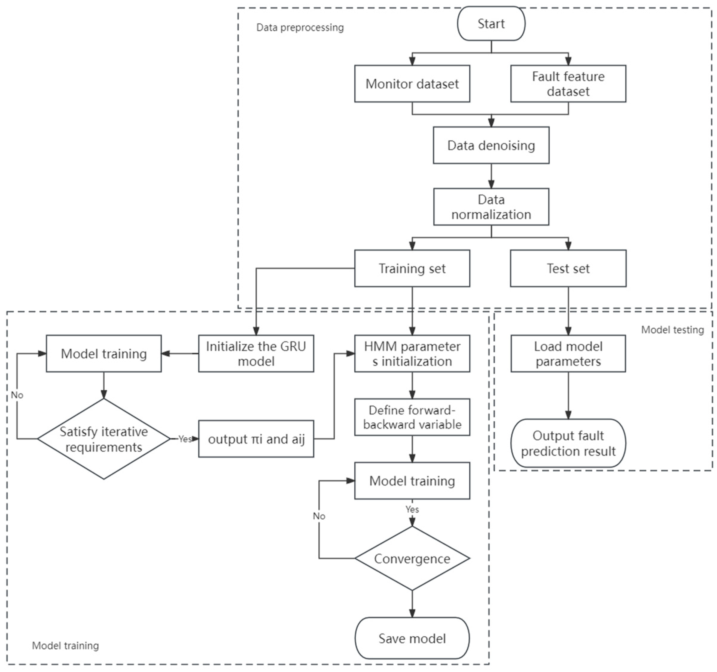
2.4. GRU-HMM Fault Prediction Model Algorithm Flow

The algorithm flow of the GRU-HMM fault prediction modeling algorithm for the EMU gearbox is shown in Figure 1.

(1) Perform wavelet de-noising and normalization on the operation monitoring data samples O = {o₁, o₂, …, o_N} and the degradation feature sets F = {f₁, f₂, …, f_N} of each component to determine the training and testing sets.

(2) Define the HMM hidden state n = 4 and initialize the parameters π₀, a₀, and b₀(v₀).

(3) Construct the GRU network model, set the number of hidden layers, M = 4. The number of GRU units in each layer, u = 128.

(4) Input the training set, optimize the network weights and parameters through iterative training, and find the optimal prediction step size and each parameter.

(5) Output the GRU training results to update the HMM parameters π_i, a_ij.

(6) Define the forward variable α_M(i),

$${\alpha }_t(i)=P(o_1,o_2,\dots ,o_t,q_t=s_i\left|\lambda \right.),1\le i\le N$$

(9)

(7) Define the backward variable β_M(i),

$${\beta }_M(i)=P(o_{t+1},o_{t+2},\dots ,o_T,q_t=s_i\left|\lambda \right.),1\le i\le N$$

(10)

(8) Perform training on the parameters of the Baum–Welch algorithm. Define the variable γ_t⁽ⁿ⁾(i), denoting the probability of being in state q_i at moment t. Define the variable ξ_m⁽ⁿ⁾(i,j), denoting the probability of being in state q_i at moment t and in state q_j at t + 1,

$${{\gamma }_t}^{(n)}(i)=\frac{{\alpha }_t(i){\beta }_t(i)}{{\displaystyle \sum _{i=1}^N{\alpha }_t(i){\beta }_t(i)}}$$

(11)

$${{\xi }_t}^{(n)}(i,j)=\frac{{\alpha }_t(i){\alpha }_{ij}(o_{t+1}){\beta }_{t+1}(j)}{{\displaystyle \sum _{i=1}^N{\displaystyle \sum _{j=1}^N{\alpha }_t(i){\alpha }_{ij}(o_{t+1}){\beta }_{t+1}(j)}}}$$

(12)

(9) Update the HMM model parameters π_i, a_ij, and b_j(v_i) again. If the values of π_i, a_ij, and b_j(v_i) have converged, the algorithm ends; otherwise, go back to (5) to continue the iteration as follows:

$${\pi }_i=\frac{{\displaystyle \sum _{n=1}^N{{\gamma }_t}^{(n)}(i)}}{N}$$

(13)

$$a_{ij}=\frac{{\displaystyle \sum _{n=1}^N{\displaystyle \sum _{t=1}^{T-1}{{\xi }_t}^{(n)}(i,j)}}}{{\displaystyle \sum _{n=1}^N{\displaystyle \sum _{t=1}^{T-1}{{\gamma }_t}^{(n)}(i)}}}$$

(14)

$$b_j(v_i)=\frac{{\displaystyle \sum _{n=1}^N{\displaystyle \sum _{t=1,o_{n=v_k}^{(n)}}^{T-1}{{\gamma }_t}^{(n)}(i)}}}{{\displaystyle \sum _{n=1}^N{\displaystyle \sum _{t=1}^{T-1}{{\gamma }_t}^{(n)}(i)}}}$$

(15)

(10) Output model $\overline{\lambda }=(\overline{\pi },\overline{A},\overline{B})$, using the test set to output the failure probabilities $P=P(O\left|\overline{\lambda }\right.)$.

3. Simulation Modeling of Dynamics for EMU Gearbox System

CRH5, incorporating French ALSTOM technology for manufacturing, is designed for a maximum speed of 250 km/h. The biggest difference between the CRH5 and other EMUs is the transmission system, which adopts the structure of a traction motor and universal shaft-mounted gearbox, in which the universal shaft is connected to the traction motor and the gearbox through the universal joints at the two ends; the structure of the CRH5 gearbox is as shown in Figure 2.

To facilitate the subsequent dynamic simulation, the model is simplified by deleting the upper and rear covers of the box as well as all bolts, nuts, and spacers, and the traction motor is replaced by a bracket to optimize the hermetic structure of the gear, axle, and box. The exploded view of the optimized gearbox modeling is shown in Figure 3.

3.1. CRH5 Gearbox Rigid–Flexible Coupling Dynamic Modeling

The rigid–flexible coupled dynamics model is employed to analyze the vibration characteristics of the universal joint, driving gear, and driven gears of the gearbox in the normal state and fault state. This model can more accurately reflect the vibration signal characteristics.

3.1.1. Theory of Rigid–Flexible Coupled Dynamics

Universal joints and gears undergoing elastic deformation need to be interpreted in terms of a relative deformation field, which must satisfy the boundary conditions of the member, and the expression is then as follows:

$$\left\{\begin{array}{c}{u}_{f1}={\displaystyle \sum _{k=1}^{\infty }{a}_k{f}_k}\\ u_{f2}={\displaystyle \sum _{k=1}^{\infty }{b}_k{g}_k}\\ u_{f3}={\displaystyle \sum _{k=1}^{\infty }{c}_k{h}_k}\end{array}\right.$$

(16)

where u_f1, u_f2, and u_f3 denote the deformation components of the flexible body coordinates (x₁, x₂, and x₃); a_k, b_k, and c_k are the coefficients with respect to time t, and f_k, g_k, and h_k are the basis functions of the deformed body.

The motion constraints of universal joints and gears need to consider elastic deformation. Their motion constraint equations are as follows:

$$\left\{\begin{array}{c}C\left(q,t\right)=0\\ C_{q}q=-C_t\\ C_q\ddot{q}=-\left[C_{tt}+\left(C_q\dot{q}\right)\ddot{q}+2C_{qt}\dot{q}\right]\end{array}\right.$$

(17)

where C is the constraint equation; $q,\dot{q},\ddot{q}$ are the velocity, position, and acceleration vectors of the flexible body; C_qq is the coordinate velocity of the flexible body; and $C_q\ddot{q}$ is the acceleration of its motion.

The CRH5 gearbox rigid–flexible coupled dynamics system is connected by constraints and force elements, and the dynamics equations of the system are as follows:

$$M^i{\ddot{q}}^i+C_{q^i}^{iT}\lambda =Q_e^i+Q_V^i, i=1,2,3$$

(18)

where M is the inertia matrix of the gearbox; λ is the Lagrange operator; Q_e is the generalized external force vector; Q_V is the generalized inertia force vector related to the velocity quadratic; and i denotes the flexible body components, i.e., the universal joints, driving gear, and driven gear.

3.1.2. Working Environment and Model Setup

The 3D model of the CRH5 gearbox is imported into ADAMS, and the material and mass properties of the solid unit are defined to realize multi-rigid body dynamics modeling of the CRH5 gearbox. Since it is necessary to analyze the vibration characteristics of the gearbox universal joints, driving gear, and driven gears in normal and fault states, the research object is softened to establish a rigid–flexible coupling dynamics model. The entire rigid–flexible coupled dynamics simulation model of the CRH5 gearbox is composed of three flexible bodies, including universal joints, the driving gear, and driven gears, and eleven rigid bodies, including the gearbox case, bushings, axles, and connecting shafts. The six bearings in the gearbox are modeled using the Adams Machinery module in ADAMS. The gearbox case and axle take one vertical degree of freedom to characterize the wheel–rail excitation; the rest of the components take three degrees of freedom in the longitudinal, transverse, and vertical directions; the whole system contains 38 rigid and flexible degrees of freedom.

The View Flex module of ADAMS can generate flexures, but the generated flexures are only oriented to simpler components, and for complex components such as gears their accuracy is greatly reduced, which is not suitable for research needs. Therefore, by using ANSYS to divide the cross joints and gears into unit meshes that satisfy the calculation accuracy, performing rigid treatment at the connection of components as connection nodes, saving the modal analysis calculation results into .mnf format files, and importing the components into ADAMS for further parameterization, the rigid–flexible coupling dynamics model of the CRH5 gearbox is constructed.

3.2. CRH5 Gearbox Rigid–Flexible Dynamics Model Contact Force Setting

3.2.1. CRH5 Gearbox Rigid–Flexible Coupling Dynamic Modeling

Using ADAMS for CRH5 gearbox rigid–flexible coupled dynamics modeling, the cross shaft and follower shaft of the universal joint, as well as the normal contact force of the active and follower gears, can be calculated by the impact function method. The impact model equates the meshing contact process as a nonlinear spring-damping model based on the depth of penetration, and the magnitude of the contact force is directly proportional to the depth of penetration and the contact stiffness. The function expression is as follows:

$$F_n=K\times {\delta }^e+step(\delta ,0,0,d_{\max },C_{\max })\frac{d\delta }{dt}$$

(19)

For the tangential contact force, the Coulomb friction method is used to calculate the force, whose magnitude is proportional to the positive pressure and whose direction is opposite to the direction of the relative slip velocity, with the following functional expression:

$$F_s=-F_n\times step(v_t,-V_S,-1,V_S,1)\times step(ABS(v_t),V_S,f_{st},V_d,f_{dy})$$

(20)

3.2.2. Contact Force Parameter Setting

According to the analysis of domestic and international studies [31,32], the parameters are set as follows:

• Modulus of elasticity E. Reflecting the stiffness of the material during elastic deformation, E = 2.07 × 10¹¹.
• Poisson’s ratio μ. Reflecting the coefficient of transverse deformation of the material in one direction, μ = 0.3.
• Contact coefficient K. Related to the shape and material properties of the contact surface, it is calculated according to Hertz contact theory, K = 1.29 × 10⁶.
• Contact index e. Reflecting the degree of nonlinearity of the material and calculated according to the Hertz contact theory, e = 1.5.
• Damping coefficient C. Reflecting the energy loss when objects collide, empirically, C = 10.
• Gear cutting depth d. Empirically, d = 0.1 mm.
• The coefficient of kinetic friction f_dy = 0.05, the kinetic slip velocity v_d = 10 mm/s, the coefficient of static friction f_st = 0.08, and the static slip velocity v_s = 1 mm/s.
• According to a related study [33], load-bearing loads and line excitation curves are incorporated at the axle.

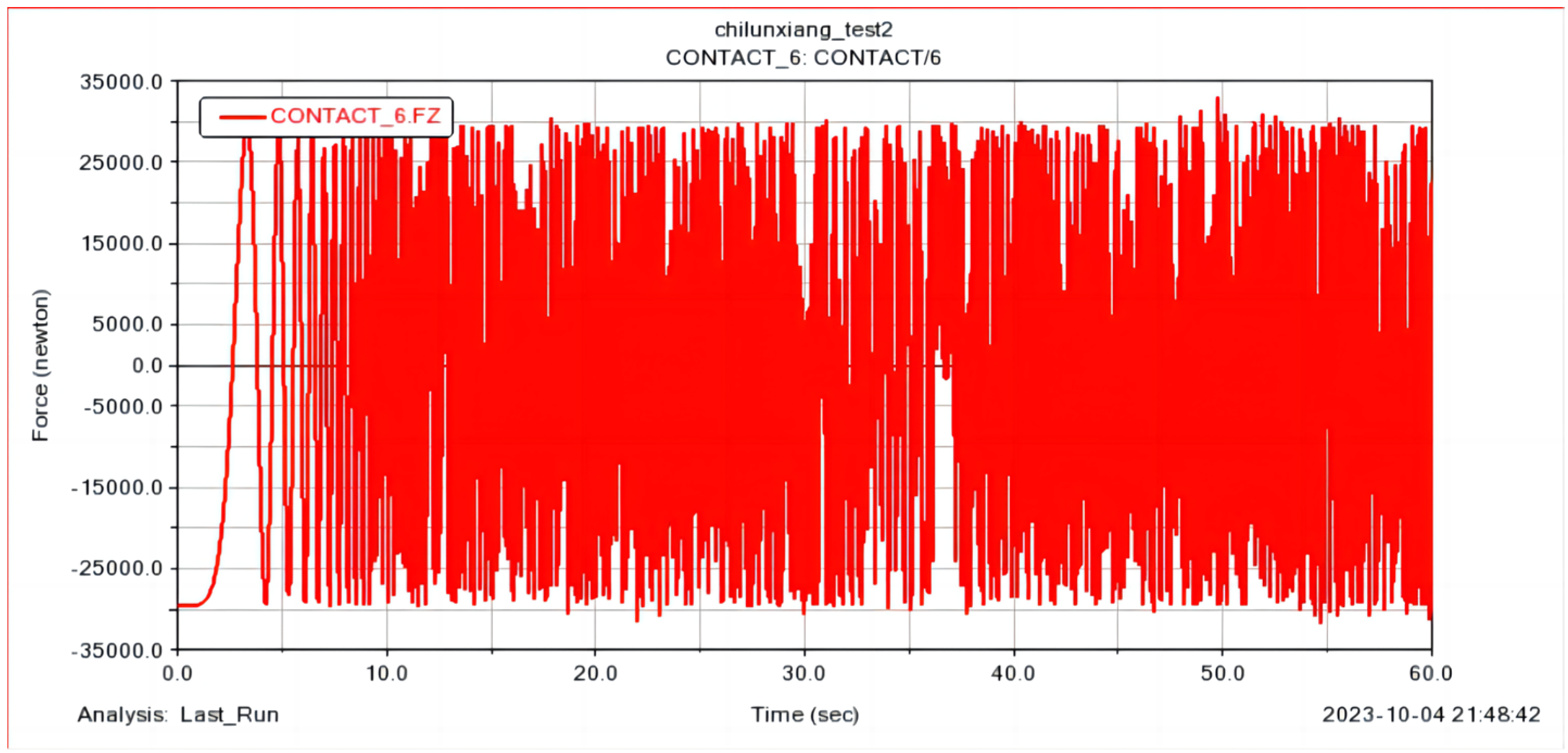
3.3. Feasibility Testing

The motor input time is 60 s and the angular velocity is 0–18,000 d/s. The gear meshing force curve is shown in Figure 4. According to related research [34], the bevel gear meshing force is about 25 KN under an approximate working condition; the simulation results are consistent with this measurement.

Then, the monitoring data of a particular train CRH5 from 9 June 2021 18:08:08 to 18:27:43 is selected for simulation. Compare the trend of the simulation results with the actual monitoring results. The traction motor angular velocity input curve during this time period is shown in Figure 5.

The vibration data from the online monitoring system of China Railway will be preprocessed, and the Root-Mean-Square (RMS) of the time-domain vibration acceleration every 5 s will be displayed as the time-domain characteristic value. After calculating the RMS of the simulated time-domain vibration acceleration and comparing the time-domain characteristic value of the actual operation, it is found that the general trends of the two coincide with each other. The actual and simulation comparisons are shown in Figure 6.

The frequency-domain vibration acceleration of the simulation is obtained using fast Fourier transform. The same treatment as the time-domain vibration acceleration is compared with the actual vibration frequency-domain eigenvalues, and the general trends of the two are found to match. The simulation and actual comparisons are shown in Figure 7.

Through the above analysis, the results of the CRH5 gearbox dynamics simulation model are basically consistent with the actual operation data, indicating the feasibility of this dynamics simulation model.

4. CRH5 Gearbox Degradation Feature Extraction and Analysis

Fault prediction of CRH5 gearbox key components requires the degradation characteristics of the key components over their full lifecycle to improve the accuracy of the prediction. Therefore, it is necessary to simulate the degradation process of key components using dynamics simulation, extract their vibration acceleration signals, calculate the vibration eigenvalues at each stage of the full lifecycle, and use the vibration eigenvalues and operation monitoring data to predict potential failures of key components.

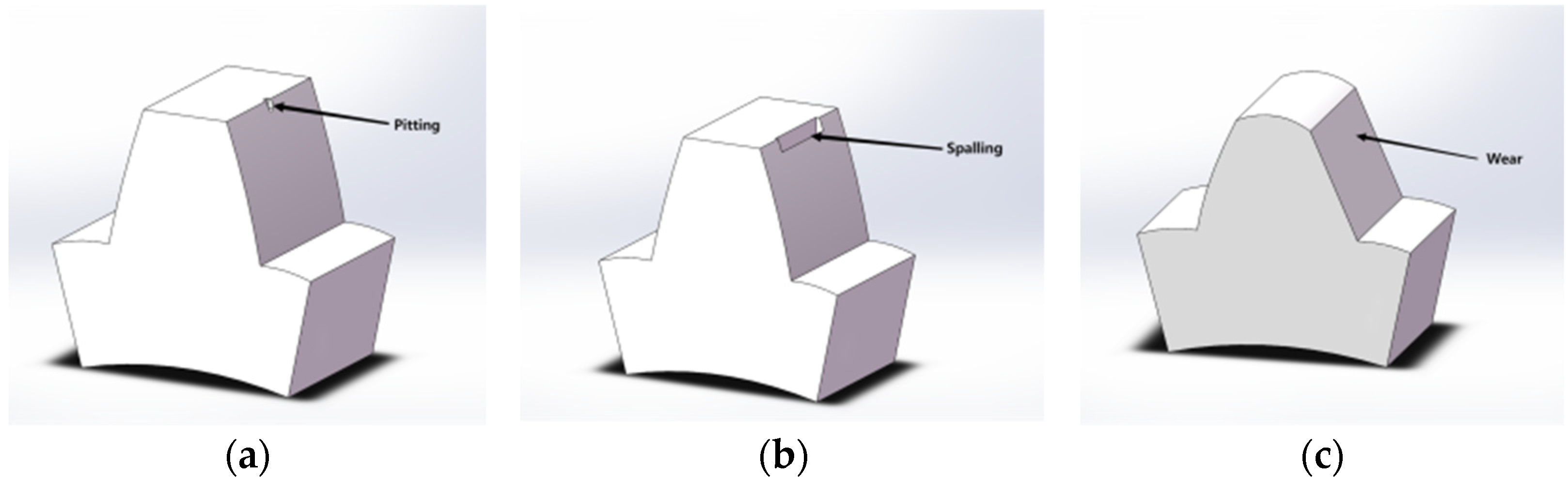
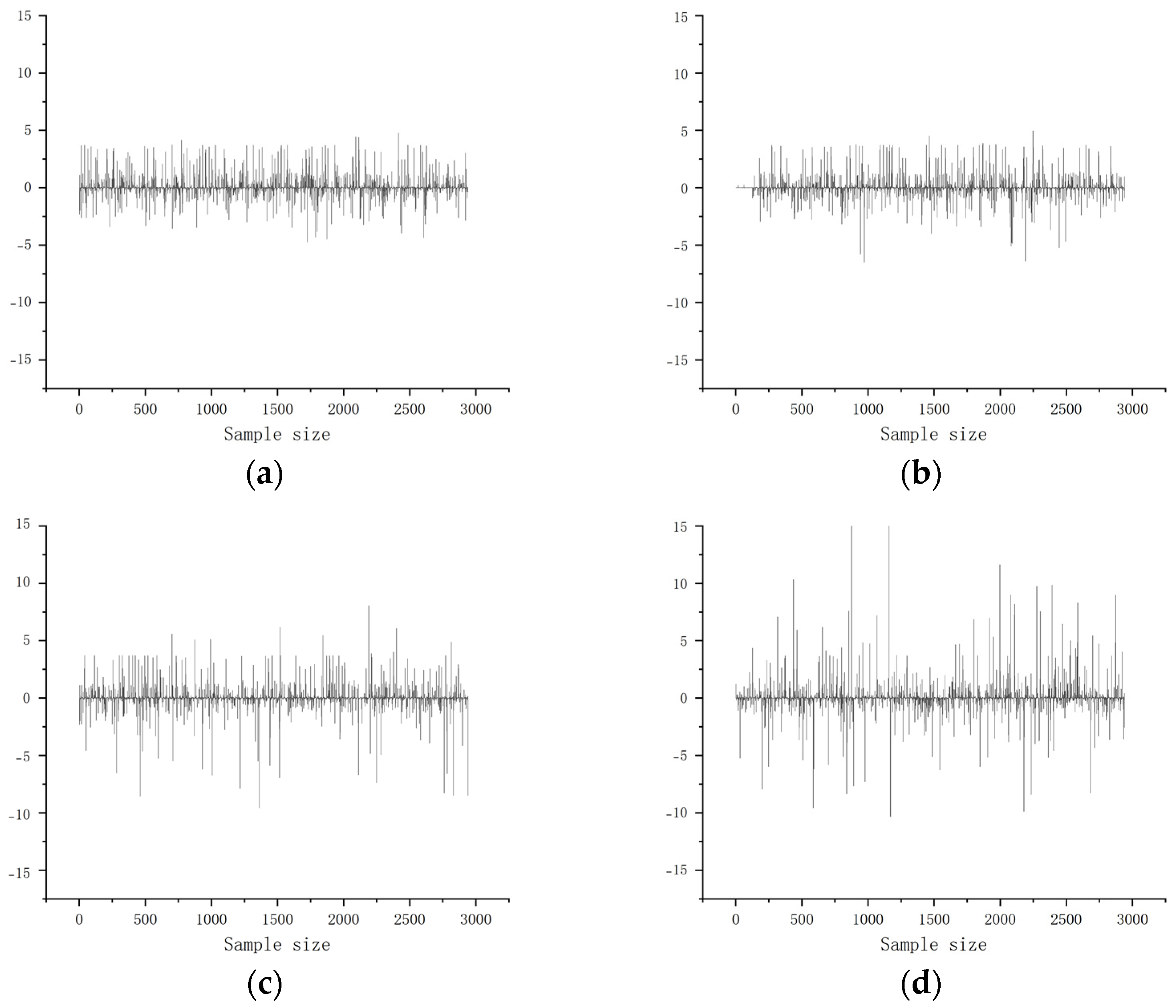
4.1. Transient Fault Simulation and Deep Learning of Critical Component Degradation Processes

To accurately describe the degradation process of the key components of the CRH5 gearbox, this study utilizes the transient process at the key stage of component degradation for dynamics simulation, extracts the time-domain vibration acceleration signals at the key stage of component degradation, and trains the degradation characteristics of the key components over the whole life cycle using deep learning.

Taking the driving gear as an example, according to the relevant literature and field research [35,36,37], the degradation process of the gear is found to be driven by pitting and spalling caused by impact-type failures, leading to the uniform wear state characteristic of stable-type failures. Figure 8 shows a schematic diagram of the key stages of degradation such as pitting, spalling, and wear of a single tooth of the driving gear. After remodeling the degradation critical stage, it is imported into ANSYS for meshing and generating a flexible body. The new flexure is imported into ADAMS to replace the normal state driving gear and a dynamic simulation is performed. Its time-domain vibration acceleration signal is extracted for training.

Since the degradation process of parts is time-sequential and there is a causal relationship between adjacent degradation stages, the training of each piece of transient fault simulation data can also be carried out using the GRU-HMM model proposed in this paper, but the model is only carried out to the initial vector update stage. A convergence optimization function F needs to be added to the GRU for gear degradation trend training,

$$F=\theta -\beta {\nabla }_{\theta }{\displaystyle {\sum }_{T_i~p(T)}{L}_{T_i}(f_{{\theta }_i})}$$

(21)

where f is the convergence function, θ is the model update gradient after training a set of tasks, β is the step size of the gated neural network, and $L_{T_i}(f_{\theta })$ is the loss of the function after the task T_i.

The training objective of GRU is to minimize the loss; the objective function and the loss function are as follows:

$$\underset{\theta }{\min }{\displaystyle {\sum }_{T_i~p(T)}{L}_{T_i}(f_{{\theta }_i})}={\displaystyle {\sum }_{T_i~p(T)}{L}_{T_i}(f_{\theta -\beta {\nabla }_{\theta }{L}_{T_i}(f_{{\theta }_i})})}$$

(22)

$$L_{T_i}(f_{\theta })={\displaystyle {\sum }_{x^j,y^j~T_i}‖f_{\theta }(x^j)-y^j‖}$$

(23)

where x^j denotes the jth data and y^j denotes the relative predicted data.

Taking the driving gear at 1500 rpm as an example, the time-domain vibration acceleration of the normal state and three degradation state simulations are shown in Figure 9. After training the GRU-HMM model, the time-domain vibration acceleration of the driving gear at 1500 rpm operating conditions for the whole life cycle is shown in Figure 10. The training model for the full lifecycle of degradation was validated using the gearbox dataset from Southeast University, comparing the relevant literature and EMU on-board monitoring data, which proved that this method is feasible [38,39].

After remodeling the critical degradation stages of the universal joints, driving gear, and driven gears, the time-domain vibration acceleration at 500 rpm intervals from 0 to 3500 rpm are calculated separately for each component. These will be used in the construction of the hybrid feature domain.

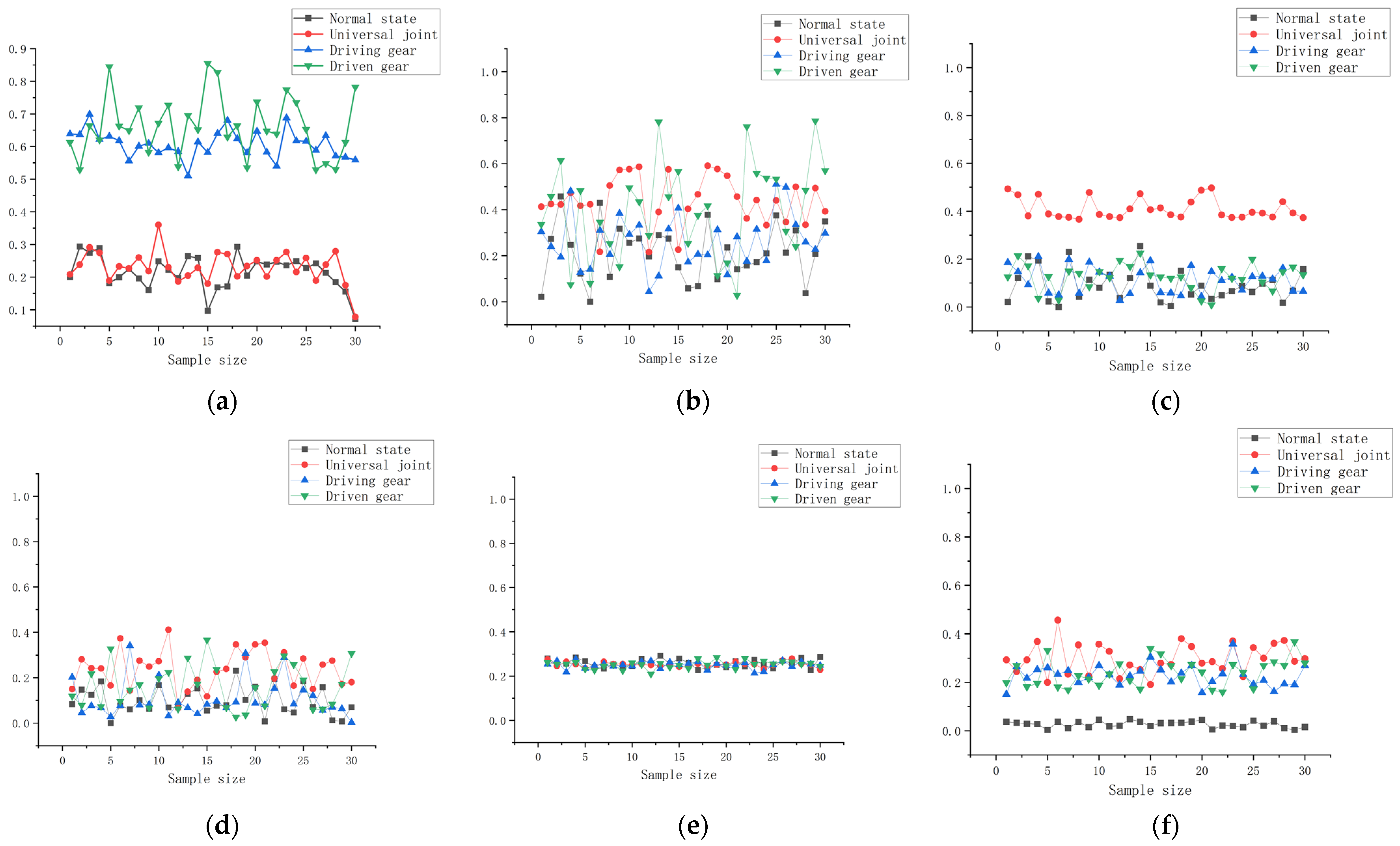
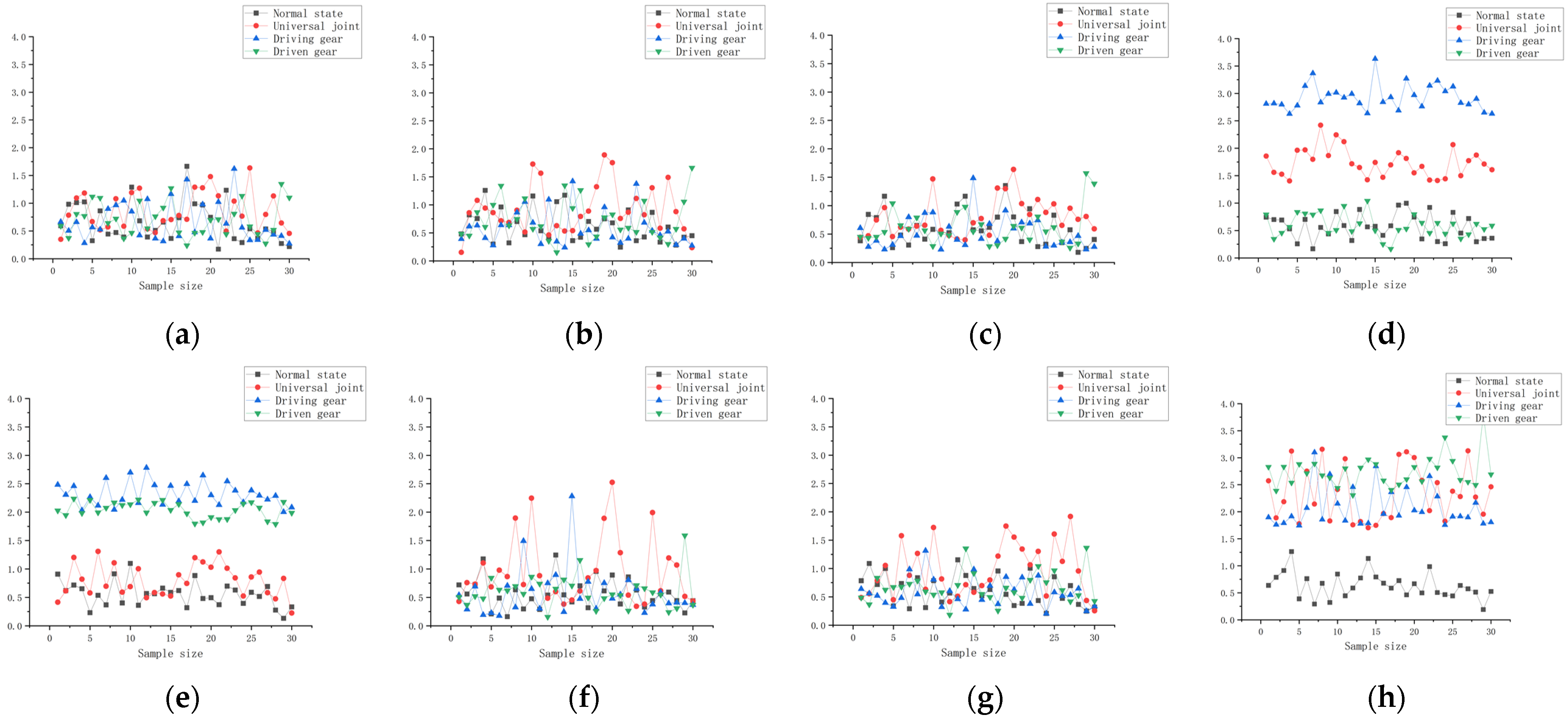
4.2. Constructing Hybrid Feature Domains

The hybrid feature domain is constituted with time-domain feature metrics, frequency-domain feature metrics, and energy distribution after wavelet packet decomposition. The time-domain and frequency-domain feature metrics are shown in

Table 1. Time-domain and frequency-domain vibration characterization metrics.

Designation	Expression (Math.)	Designation	Expression (Math.)
RMS	$X_{rms}=\sqrt{\frac{{\displaystyle \sum _{N=1}^N{x}^2(n)}}{N}}$	Pulse index	$I=\frac{\max \left|x(n)\right|}{\overline{x}}$
Margin index	$L=\frac{\max \left|x(n)\right|}{X_{rms}}$	Gravity frequency	$F_c=\frac{{\displaystyle \sum _{n=1}^N{f}_n\cdot s(n)}}{{\displaystyle \sum _{n=1}^{N}s(n)}}$
Kurtosis index	$K=\frac{{{\displaystyle \sum _{n=1}^N\left[x(n)-\overline{x}\right]}}^4}{(N-1){\sigma }_x^4}$	RMS frequency	$F_r=\sqrt{\frac{{\displaystyle \sum _{n=1}^N{f}_n^2\cdot s(n)}}{{\displaystyle \sum _{n=1}^{N}s(n)}}}$

where x(n) is the time-domain sequence of the vibration signal, $\overline{x}$ is the mean value of x(n), s(n) is the spectrum of the signal x(n), and f_n is the frequency value of the nth spectral line.

.

Wavelet packet decomposition is a time-frequency domain feature extraction algorithm that is able to observe frequency information in a small area of the frequency domain. Let $s_{j,k}(i)$ be the reconstructed signal of the kth band of the jth layer obtained after wavelet packet decomposition of the original signal; then, its corresponding energy $E_{j,k}$ is as follows:

$$E_{j,k}={\displaystyle \int {\left|s_{j,k}(t)\right|}^2}dt={\displaystyle \sum _{i=1}^N{\left|s_{j,k}(i)\right|}^2}$$

(24)

where N is the length of the signal, k is the ordinal number of the sub-bands of the wavelet packet in layer j, and the number of sub-bands is M = 2j. E_j and W_j are the energy and eigenvectors of each sub-band in layer j.

$$E_j={\displaystyle \sum _{k=0}^{M-1}{E}_{j,k}}$$

(25)

$$W_j=\frac{{\left[E_{j,0},E_{j,1},\dots ,E_{j,M-1}\right]}^T}{E_j}$$

(26)

Setting the wavelet packet decomposition layer to 3, W3 is an eight-dimensional vector, which, together with the six-dimensional time-frequency domain feature metrics described above, contributes to a fourteen-dimensional hybrid feature domain.

4.3. Hybrid Feature Domain Sensitivity Analysis

Taking a 1500 rpm working condition as an example, there are 3000 sampling points of vibration acceleration in the normal state and degradation process of the key components of the gearbox, and every 100 sampling points of each state type are intercepted as a sample, for a total of 30 samples for each state type. The six characteristic indexes in time and frequency domains are calculated, respectively, and, after normalizing the calculation results, the comparison diagrams of normal state and degradation positions are shown in Figure 11. Among them, the RMS, kurtosis index, and RMS frequency have better sensitivity to component degradation, but they cannot be accurately differentiated for fault location.

The wavelet packet decomposition feature indexes of 30 samples for each state are calculated, and the feature indexes are compared in Figure 12. Among them, W(3,3), W(3,4), and W(3,7) are more sensitive to degradation and can be effectively separated from different locations by combining the RMS, kurtosis index, and RMS frequency. Therefore, these six feature indicators are selected to construct a six-dimensional hybrid feature domain. The remaining feature indicators with low sensitivity are eliminated.

The full lifecycle degraded hybrid feature domain of CRH5 gearbox key components is set in the preprocessing stage of the GRU-HMM fault prediction model. Before fault prediction, the operation monitoring data are noise reduced and the six-dimensional hybrid feature domain is calculated. The RMS, kurtosis index, and RMS frequency during operation are compared with the full lifecycle degradation hybrid feature domain to determine the initial probability of failure π. Then, the eigenvalues of W(3,3), W(3,4), and W(3,7) are used to determine the location of the hidden failure, and the initial probability parameter is updated by the GRU to perform the failure prediction.

5. Instance Verification

5.1. Source of Experimental Data

The verification data come from the operation monitoring data of a CRH5 within 30 days before advanced repair in an EMU depot of China Railway. This CRH5 had undergone a life-critical replacement of the driving gear and driven gears of the gearbox system during this advanced repair. Thus, this dataset has better verification for GRU-HMM fault prediction and hidden fault judgment.

Because of the large number of operational monitoring data entries, the low-speed monitoring data resulting from transitions or waiting were deleted, and the monitoring data for every 48 h were used as a set of samples, totaling 15 sets of samples. Wavelet packet noise reduction was applied to all sample data, using the first ten sets of samples as the training set and the last five sets as the test set for fault prediction of the CRH5 gearbox.

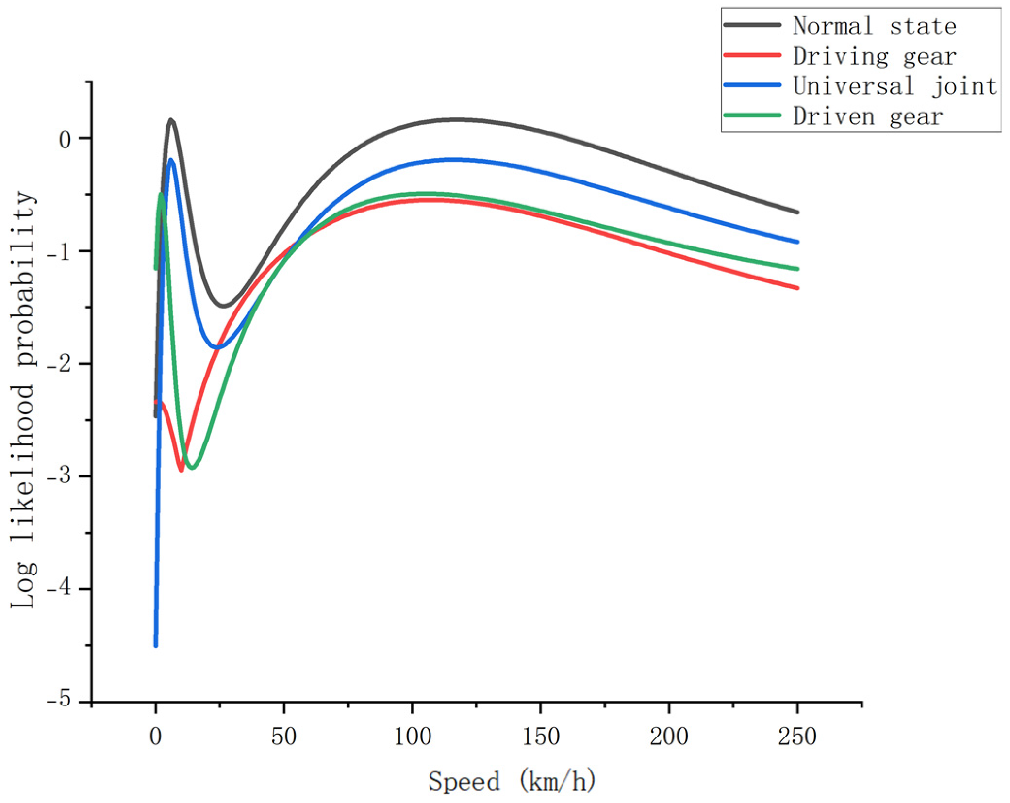
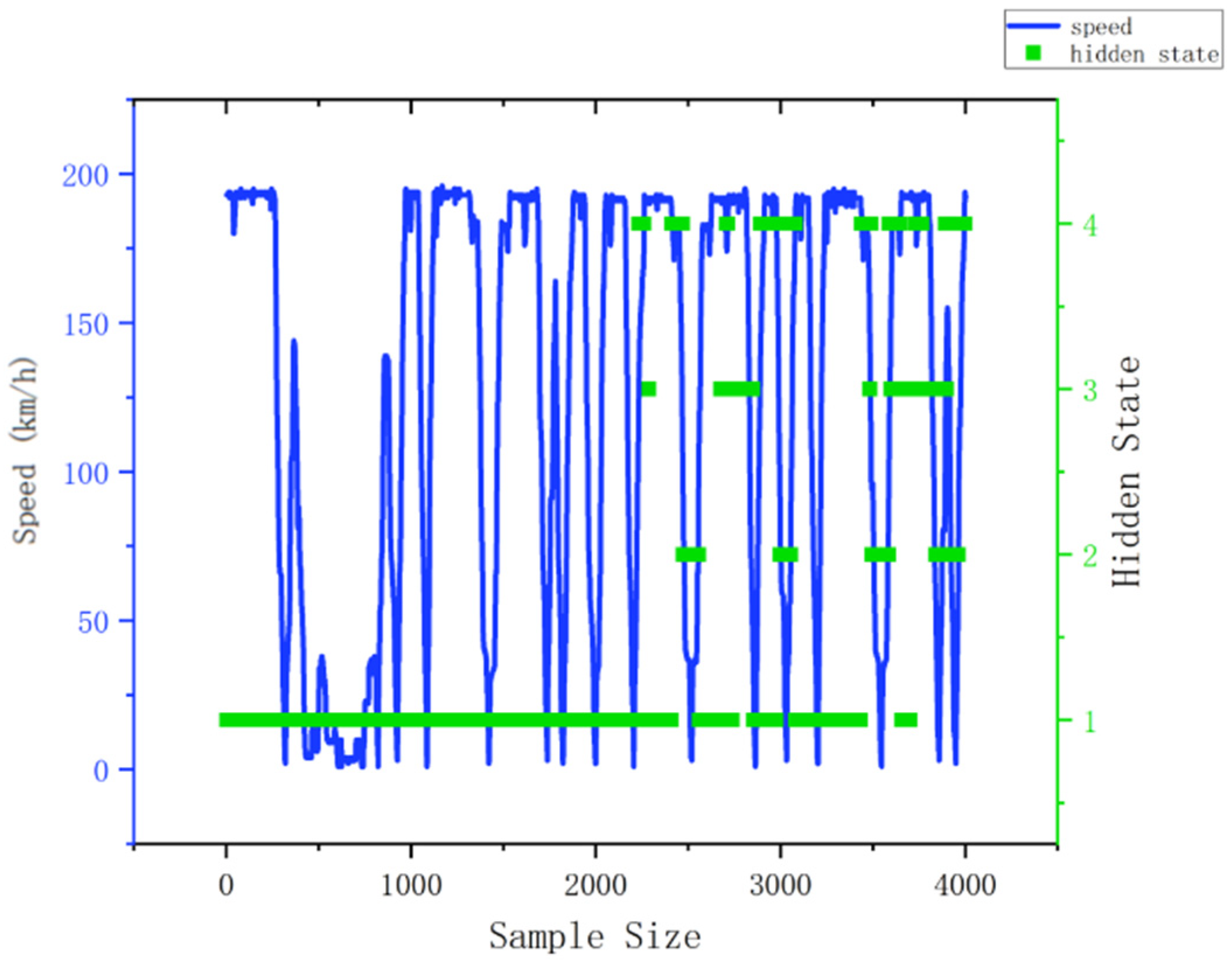
5.2. Verification of GRU-HMM Fault Prediction Model

The HMM initial vector, state transfer matrix, and confusion matrix are first calculated from the training set with the following values:

$$\pi =\left[0.782,0.115,0.06,0.025,0.018\right];$$

$$A=\left[\begin{array}{cccc}0.9530& 0& 0.0118& 0.0352\\ 0& 0.9855& 0.0145& 0\\ 0.0097& 0.0179& 0.9470& 0.0255\\ 0.0822& 0& 0.0254& 0.8925\end{array}\right];$$

$$B=\left\{\begin{array}{cc}\left[\begin{array}{cc}18.5143& 0.1184\\ 0.1184& 0.0508\end{array}\right]& \left[\begin{array}{cc}654.462& 4.5942\\ 4.5942& 0.0551\end{array}\right]\\ \left[\begin{array}{cc}526.172& 1.82\\ 1.82& 0.0967\end{array}\right]& \left[\begin{array}{cc}569.049& -8.9019\\ -8.9019& 0.4765\end{array}\right]\end{array}\right\}$$

The hybrid feature domain is substituted into the GRU for feature fusion, and the initial vectors and state transfer matrices are updated. The log-likelihood probabilities of the initial vector updates for each hidden fault type are shown in Figure 13. Where the log-likelihood probability of the driving gear increases at increasing speed levels, especially at high speeds, the risk of failure of the driving gear increases. The log-likelihood probability of the universal joint has the highest risk of failure at moderate speeds. The log-likelihood probability of the universal joint has the highest risk of failure at moderate speeds. The log-likelihood probability of the driven gear is higher at lower speeds, decreases with increasing speed, and then increases again at higher speeds, indicating that the risk of failure of the driven gear is higher at low- and high-speed operations.

The updated initial vectors and state transfer matrices are substituted into the GRU-HMM for training. The probability distribution of hidden states is calculated using the test set, and the results are normalized to obtain the fault prediction results for each type of failure mode. The results of the velocity–hidden state distribution for one of the sample sets of the test set are shown in Figure 14. The probability of hidden failures of the driving gear and driven gears is higher from the figure. Through the maintenance records of the EMU undergoing advanced repairs in the manufacturing plant, comparing the replaced gear sets, it is proven that the predicted results match the actual results, and the feasibility of the GRU-HMM fault prediction model is demonstrated.

5.3. Comparative Analysis

To verify the advantage of the proposed fault prediction method in terms of its fault identification accuracy, the traditional HMM and SVM diagnostic models were compared for the prediction of EMU gearbox faults. The recognition accuracies of the four degraded positions are shown in

Table 2. Comparison of recognition accuracy of various fault prediction methods.

Model	Normal State	Universal Joint	Driving Gear	Driven Gear	Recognition Times (min)
GRU-HMM	0.988	0.9	0.975	0.975	7.5
HMM	0.912	0.622	0.683	0.725	2.3
SVM	0.925	0.883	0.875	0.875	3.1

. The recognition accuracy of GRU-HMM was found to be significantly higher than that of the traditional HMM and SVM methods. However, a higher recognition time compared to the other two methods was observed due to the fact that this method requires multiple trainings for the hybrid feature domain, initial vector, and state transfer matrix.

6. Conclusions

• A model for predicting faults in the CRH5 gearbox has been developed by establishing a dynamic coupling dynamics model and utilizing vibration acceleration data from key components throughout the gearbox’s degradation process. By creating a six-dimensional degradation hybrid feature domain, the issue of extracting fault features with limited CRH5 gearbox fault samples is addressed. The hybrid feature domains obtained through dynamics simulation also have some limitations. For example, the simulation data are not generalized enough to fully simulate the data fluctuations caused by wheel–rail excitation during EMU operation, and the performance of the model in the real environment cannot be fully evaluated. The accelerated life test of key gearbox components will be utilized to compensate for the above shortcomings in the subsequent study.
• The proposed GRU-HMM CRH5 gearbox fault prediction model combines the strengths of HMM in handling time-series data with GRU to overcome limitations on input sequence length, enhancing its ability to handle long-range dependency data. The effectiveness of the GRU-HMM fault prediction model was confirmed using operational monitoring data from a CRH5 prior to advanced repair and actual overhaul component records. Compared to traditional fault prediction models like HMM and SVM, the combined accuracy of the GRU-HMM model was found to be 15% higher.
• Although the GRU-HMM fault prediction model improves the recognition accuracy, it requires a large number of calculations in the preprocessing and training phases of the monitoring data, resulting in time-consuming fault prediction. In the subsequent study, the hyperparameters of the model will be adjusted to find the optimal combination of parameters to reduce the computation time. Cross-scale fault prediction studies of EMU gearboxes at a material scale and structural scale will also be considered, combining the multi-physical field coupling effect of temperature–vibration–load and performing comprehensive analysis to improve the accuracy of fault prediction.

References

1. Inturi, V.; Sabareesh, G.R.; Sharma, V. Integrated Vibro-Acoustic Analysis and Empirical Mode Decomposition for Fault Diagnosis of Gears in a Wind Turbine. Procedia Struct. Integr. 2019, 14, 937–944. [Google Scholar] [CrossRef]
2. Yang, Y.; Li, X.; Pan, H.; Cheng, J. A composite fault feature extraction method for rotating machinery based on nonlinear mode decomposition. China Mech. Eng. 2018, 29, 7. [Google Scholar]
3. Wang, Z.; Wang, J.; Zhang, J.; Zhao, Z.; Kou, Y. Based on improved MOMEDA for gearbox composite fault diagnosis. Vibration. Test. Diagn. 2018, 38, 6. [Google Scholar]
4. Singh, P. Novel Fourier quadrature transforms and analytic signal representations for nonlinear and non-stationary time-series analysis. R. Soc. Open Sci. 2018, 5, 181131. [Google Scholar] [CrossRef] [PubMed]
5. Rakesh, A.; Aravind, A.; Narendiranath, B.T.; Jahzan, M. Application of EMD ANN and DNN for Self-Aligning Bearing Fault Diagnosis. Arch. Acoust. J. Pol. Acad. Sci. 2018, 43, 163–175. [Google Scholar] [CrossRef] [PubMed]
6. Kumar, P.S.L.A. Selecting effective intrinsic mode functions of empirical mode decomposition and variational mode decomposition using dynamic time warping algorithm for rolling element bearing fault diagnosis. Trans. Inst. Meas. Control 2019, 41, 1923–1932. [Google Scholar] [CrossRef]
7. Michau, G.; Fink, O. Unsupervised Fault Detection in Varying Operating Conditions. In Proceedings of the 2019 IEEE International Conference on Prognostics and Health Management 2019 (PHM 2019—San Francisco), San Francisco, CA, USA, 17–20 June 2019. [Google Scholar]
8. Fujita, Y.; Nagarajan, P.; Kataoka, T.; Ishikawa, T. ChainerRL: A Deep Reinforcement Learning Library; Cornell University Library: Ithaca, NY, USA, 2021. [Google Scholar]
9. Li, X.; Xu, H.; Zhang, J.; Chang, H.H. Deep Reinforcement Learning for Adaptive Learning Systems. J. Educ. Behav. Stat. 2023, 48, 220–243. [Google Scholar] [CrossRef]
10. Morales, E.F.; Murrieta-Cid, R.; Becerra, I.; Esquivel-Basaldua, M.A. A survey on deep learning and deep reinforcement learning in robotics with a tutorial on deep reinforcement learning. Intell. Serv. Robot. 2021, 14, 773–805. [Google Scholar] [CrossRef]
11. Zhang, Z.; Zhang, X.; Zhang, P.; Wu, F.; Li, X. Gearbox Composite Fault Diagnosis Method Based on Minimum Entropy Deconvolution and Improved Dual-Tree Complex Wavelet Transform. Entropy 2018, 21, 18. [Google Scholar] [CrossRef] [PubMed]
12. Guo, J.; Si, Z.; Xiang, J. A compound fault diagnosis method of rolling bearing based on wavelet scattering transform and improved soft threshold denoising algorithm. Measurement 2022, 196, 111276. [Google Scholar] [CrossRef]
13. Tutivén, C.; Vidal, Y.; Insuasty, A.; Campoverde-Vilela, L.; Achicanoy, W. Early Fault Diagnosis Strategy for WT Main Bearings Based on SCADA Data and One-Class SVM. Energies 2022, 15, 4381. [Google Scholar] [CrossRef]
14. Yao, D.; Yang, J.; Cheng, X.; Wang, X. Research on Bearing Fault Diagnosis Based on Multiscale Intrinsic Mode Permutation Entropy and SA-SVM. J. Mech. Eng. 2018, 9, 168–176. [Google Scholar] [CrossRef]
15. Chen, J.; Jiang, J.; Guo, X.; Tan, L. An Efficient CNN with Tunable Input-Size for Bearing Fault Diagnosis. Int. J. Comput. Intell. Syst. 2021, 14, 625–634. [Google Scholar] [CrossRef]
16. Rao, M.; Zuo, M.J. In A New Strategy for Rotating Machinery Fault Diagnosis under Varying Speed Conditions Based on Deep Neural Networks and Order Tracking. In Proceedings of the 2018 17th IEEE International Conference on Machine Learning and Applications (ICMLA), Orlando, FL, USA, 17–20 December 2018. [Google Scholar]
17. An, Z.; Li, S.; Wang, J.; Xin, Y.; Xu, K. Generalization of deep neural network for bearing fault diagnosis under different working conditions using multiple kernel method. Neurocomputing 2019, 352, 42–53. [Google Scholar] [CrossRef]
18. Li, X.; Li, J.; Qu, Y.; He, D. Semi-Supervised Gear Fault Diagnosis Using Raw Vibration Signal Based on Deep Learning. Chin. J. Aeronaut. 2019, 33, 418–426. [Google Scholar] [CrossRef]
19. Peng, B.; Xia, H.; Lv, X.; Annor-Nyarko, M.; Zhang, J. An intelligent fault diagnosis method for rotating machinery based on data fusion and deep residual neural network. Appl. Intell. 2021, 52, 3051–3065. [Google Scholar] [CrossRef]
20. He, Z.; Shao, H.; Zhang, X.; Cheng, J.; Yang, Y. Improved Deep Transfer Auto-Encoder for Fault Diagnosis of Gearbox under Variable Working Conditions with Small Training Samples. IEEE Access 2019, 7, 115368–115377. [Google Scholar] [CrossRef]
21. Krummenacher, G.; Ong, C.S.; Koller, S.; Kobayashi, S.; Buhmann, J.M. Wheel Defect Detection with Machine Learning. IEEE Trans. Intell. Transp. Syst. 2017, 19, 1176–1187. [Google Scholar] [CrossRef]
22. Yang, B.; Lei, Y.; Jia, F.; Xing, S. An intelligent fault diagnosis approach based on transfer learning from laboratory bearings to locomotive bearings. Mech. Syst. Signal Process. 2019, 122, 692–706. [Google Scholar] [CrossRef]
23. Wang, N.; Jiang, D. Vibration response characteristics of a dual-rotor with unbalance-misalignment coupling faults: Theoretical analysis and experimental study. Mech. Mach. Theory 2018, 125, 207–219. [Google Scholar] [CrossRef]
24. Karlsson, H.; Qazizadeh, A.; Stichel, S.; Berg, M. Research on Status Monitoring of Suspension Components in Rail Vehicles Based on Machine Learning Methods. Smart Rail Transit 2022, 59, 72–76. [Google Scholar]
25. Fu, Y.; Huang, D.; Qin, N.; Liang, K.; Yang, Y. High-Speed Railway Bogie Fault Diagnosis Using LSTM Neural Network. In Proceedings of the 2018 37th Chinese Control Conference (CCC), Wuhan, China, 25–27 July 2018. [Google Scholar]
26. Liang, K.; Qin, N.; Huang, D.; Fu, Y. Convolutional Recurrent Neural Network for Fault Diagnosis of High-Speed Train Bogie. Complexity 2018, 2018, 4501952. [Google Scholar] [CrossRef]
27. Huang, D.; Fu, Y.; Qin, N.; Gao, S. Fault diagnosis of high-speed train bogie based on LSTM neural network. Chin. Sci. 2021, 64, 256–258. [Google Scholar] [CrossRef]
28. Wang, H.; Men, T.; Li, Y. Transformer for High-Speed Train Wheel Wear Prediction with Multiplex Local-Global Temporal Fusion. IEEE Trans. Instrum. Meas. 2022, 71, 1–12. [Google Scholar] [CrossRef]
29. Cheng, C.; Qiao, X.; Fu, C.; Wang, W.; Yin, X. Fault Prediction of High-Speed Train Running Gears Based on Hidden Markov Model and Analytic Hierarchy Process. In Proceedings of the 2019 CAA Symposium on Fault Detection, Supervision and Safety for Technical Processes (SAFEPROCESS), Xiamen, China, 5–7 July 2019. [Google Scholar]
30. Schmidt, K.; Hoffmann, K.H. Modified Baum Welch Algorithm for Hidden Markov Models with Known Structure. In Proceedings of the International Conference on Intelligent Human Systems Integration, San Diego, CA, USA, 7–10 February 2019. [Google Scholar]
31. Zhu, H. Research on Vibration Characteristics and Fatigue Failure of Gearbox Box of High Speed EMU. Ph.D. Thesis, Southwest Jiaotong University, Chengdu, China, 2019. [Google Scholar]
32. Gao, G.; Zhang, J.; Guo, W.; Xia, Z. Research on Fault Characteristics of Gear Box Broken Teeth in High Speed Train Based on ADAMS. Def. Transp. Eng. Technol. 2020, 18, 5. [Google Scholar]
33. Song, W. Research on Wheel Rail Load Characteristics and Track Excitation of Standard High-Speed Trains. Ph.D. Thesis, Beijing Jiaotong University, Beijing, China, 2020. [Google Scholar]
34. Liao, P. A Calculation Model for Mesh Stiffness of Spiral Bevel Gears and Research on Vibration Characteristics of Transmission Systems. Ph.D. Thesis, Chongqing University, Chongqing, China, 2019. [Google Scholar]
35. Lo, C.C.; Lee, C.H.; Huang, W.C. Prognosis of Bearing and Gear Wears Using Convolutional Neural Network with Hybrid Loss Function. Sensors 2020, 20, 3539. [Google Scholar] [CrossRef] [PubMed]
36. Deutsch, J.; He, D. Using Deep Learning-Based Approach to Predict Remaining Useful Life of Rotating Components. IEEE Trans. Syst. Man Cybern. Syst. 2017, 48, 11–20. [Google Scholar] [CrossRef]
37. Liu, H.K.; Ding, K.; He, G.L.; Li, W.H.; Lin, H.B. Research on the prediction method of gear remaining service life by combined failure mechanism and convolutional neural network. J. Mech. Eng. 2024. Available online: http://kns.cnki.net/kcms/detail/11.2187.th.20240322.1652.020.html (accessed on 27 April 2024).
38. Shao, S.; Mcaleer, S.; Yan, R.; Baldi, P. Highly Accurate Machine Fault Diagnosis Using Deep Transfer Learning. IEEE Trans. Ind. Inform. 2019, 15, 2446–2455. [Google Scholar] [CrossRef]
39. Zhang, L.; Huang, J.; Wu, R.Z.; Song, C.Y.; Wang, C.-B. A time-series reconstruction model for gear performance degradation assessment. Mech. Sci. Technol. 2022, 41, 1860–1868. [Google Scholar]
Figure 1. GRU-HMM fault prediction model flowchart.
Applsci 14 05320 g001
Figure 2. CRH5 gearbox structure.
Applsci 14 05320 g002
Figure 3. Simplified 3D model of the CRH5 gearbox.
Applsci 14 05320 g003
Figure 4. The gear meshing force curve.
Applsci 14 05320 g004
Figure 5. Input angular velocity curve.
Applsci 14 05320 g005
Figure 6. Comparison of actual and simulation time-domain curves.
Applsci 14 05320 g006
Figure 7. Comparison of actual and simulation frequency-domain curves.
Applsci 14 05320 g007
Figure 8. Critical stages of a single tooth degradation of driving gear. (a) Pitting; (b) spalling; (c) wear.
Applsci 14 05320 g008
Figure 9. Time-domain vibration acceleration in the normal state and in various degraded states. (a) Normal; (b) pitting; (c) spalling; (d) wear.
Applsci 14 05320 g009
Figure 10. Time-domain vibration acceleration over the full lifecycle of driving gear (1500 rpm).
Applsci 14 05320 g010
Figure 11. Comparison of time and frequency domain feature metrics. (a) RMS; (b) margin index; (c) kurtosis index; (d) pulse index; (e) gravity frequency; (f) RMS frequency.
Applsci 14 05320 g011
Figure 12. Comparison of wavelet packet decomposition feature metrics. (a) W(3,0); (b) W(3,1); (c) W(3,2); (d) W(3,3); (e) W(3,4); (f) W(3,5); (g) W(3,6); (h) W(3,7).
Applsci 14 05320 g012
Figure 13. Initial vector log-likelihood probabilities for each hidden fault type.
Applsci 14 05320 g013
Figure 14. The results of the velocity–hidden state distribution.
Applsci 14 05320 g014