Design and Control of a Pneumatic Muscle Servo Drive Applied to a 6-DoF Parallel Manipulator

Abstract

This article is a continuation of research on the possibility of using artificial pneumatic muscles to drive a parallel manipulator with six degrees of freedom. The authors present an artificial pneumatic muscle they have developed. The article contains a description of the research methodology and a description of the authors’ research position. The article presents the results of a comparison of the developed pneumatic muscle with an existing commercial solution. Then, the dynamic characteristics of the authors’ muscle are presented. A mathematical model is proposed that contains two inputs—the force generated by the muscle and the position of the muscle—and one output—the value of the signal controlling the pressure valve. The results of verification of the developed model are presented. The model is then presented in two versions. The first one contains the full dynamic model. The second one is its simplified version: the static model. The authors compare both models and present the comparison results. A servo drive is then synthesized and consists of a pair of muscles capable of generating the desired angular position and intended to drive a single arm of a parallel manipulator. The developed servo drive is verified on a test stand, and its behavior is assessed and analyzed in the context of its use in the manipulator.

1. Introduction

This article continues the description of work on the development of a delta-type parallel manipulator with six degrees of freedom and powered by proprietary pneumatic muscles. In the initial work [1], a comprehensive introduction to pneumatic muscles was provided, the research setup used for conducting experiments was described, and the construction of the proprietary muscle was presented. Additionally, in [1], the procedure for determining the static characteristics of the muscle and the characteristics themselves were outlined. The primary focus of [1] was on describing the process of determining the first mathematical model of the muscle, which describes the force generated by the muscle, as well as the description and results of research on the developed muscle servo drive. This drive consists of two muscles working in opposition and is used to generate the desired torque. Therefore, it can be used to drive a single arm of a parallel manipulator and can be utilized in situations where the manipulator is force-controlled. This article is the second in a series of three papers on the aforementioned topic. It provides an introduction to what pneumatic muscles are and their history and structure. Brief information about the developed muscle is presented to facilitate the reader’s understanding of the research context. A concise description of the research setup and methodology for determining the static characteristics of the muscle is also provided; a comprehensive description of these topics can be found in [1]. Next, a comparison between the proprietary muscle and Festo’s muscle is presented, justifying the use of the proprietary muscle. The subsequent section outlines the process and results of determining the dynamic characteristics of the muscle along with the controlling valve. A dynamic functional model describing the muscle position change in response to the control signal with a known load force is presented. Then, the process of synthesizing a muscle servo drive capable of achieving a desired angular position and the results of its testing are provided. The conclusion of the paper includes an assessment of the quality of the developed servo drive and its suitability for driving a single arm of a parallel manipulator under positional control.

2. Materials and Methods

2.1. Research Methodology

A pneumatic muscle is a type of single-acting cylinder that, under the influence of increased internal pressure, increases its volume by expanding its diameter while simultaneously reducing its length. The change in cylinder length is treated as the working motion [1]. The primary physical quantities describing the behavior of the muscle in a steady state are the internal pressure p, the muscle length x, and the force generated by the muscle F. Currently, pneumatic muscles are primarily offered by two companies: since 1987, the Shadow Robot Company has been involved in the production and sale of muscles based on the McKibben design, while in 1999, the well-known pneumatic equipment manufacturer Festo introduced to the market pneumatic muscles than can be customized for individual applications. They fundamentally differ in construction from the McKibben muscle. In the Festo design, the braid and rubber bladder are bonded along the entire length of the muscle. Figure 1 illustrates views of the pneumatic muscle developed by the authors at an internal pressure of $p=0.6$ MPa and at zero internal pressure.

The first stage of pneumatic muscle analysis often involves determining their static characteristics in the form of isobaric, isotonic, and isometric characteristics. The next stage is to determine the dynamic characteristics in the form of the muscle length–time relationship in response to a step change in internal pressure and with a constant muscle load force. The methodology for their determination and the characterization of muscles based on the McKibben design, Festo muscles, and many original designs have been presented, among others, as described earlier [2,3,4,5,6,7,8,9,10,11,12,13]. In the article [6], Takosoglu and colleagues presented a research methodology and determined the static characteristics—isobaric, isotonic, and isometric—of Festo pneumatic (Esslingen am Neckar, Germany) muscles and Shadow Robot Company (London, UK) muscles.In publications describing static muscle models, research mainly focuses on determining the relationship between internal pressure, muscle length, and the force generated by the muscle in relation to the muscle’s geometric parameters. Studies have also been conducted to determine dynamic models of McKibben and Festo muscles, as well as of other structures developed in various research centers, and on the development of position and force control methods using the presented mathematical models. These issues have been extensively discussed in works such as [14,15,16,17,18,19]. Due to significant friction between the fibers of the braid and between the braid and the rubber bladder, hysteresis occurs in muscles based on the McKibben design. This phenomenon applies to both muscle shortening and the force generated by it. In the case of shortening, hysteresis manifests as the difference between the contraction value at a given internal pressure and constant load force when increasing the internal pressure and the contraction value at the same internal pressure and constant load force when decreasing the pressure. When analyzing the force generated by the muscle, hysteresis refers to the difference between the force produced at a given internal pressure and constant contraction when pressure increases and the force produced at the same internal pressure and constant contraction when pressure decreases. This issue is the subject of numerous studies, including [20,21,22,23,24,25,26].

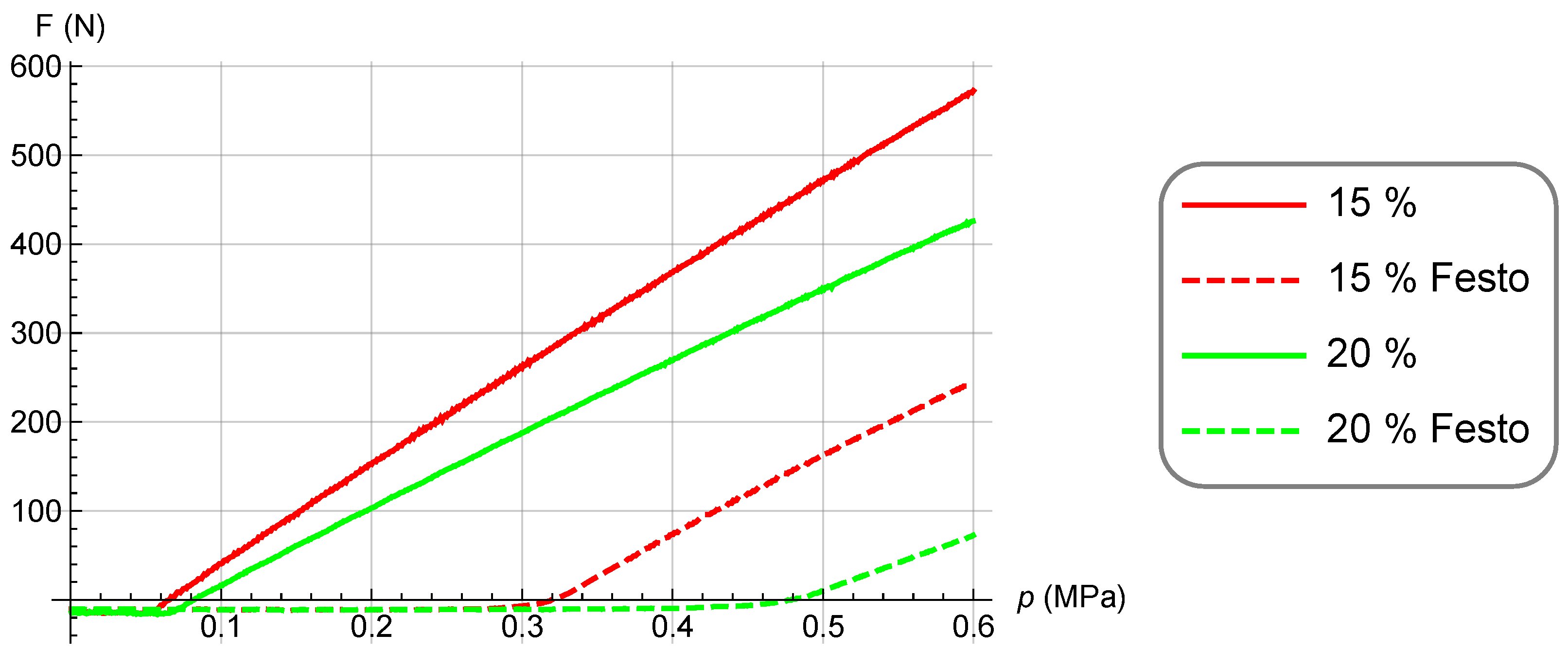
2.2. Comparison with Commercial Muscles

For the purposes of pneumatic muscle research, a research setup was developed. A comprehensive description of it can be found in [1]. Below are the most important details and the appearance of the developed setup (Figure 2).

The setup allows for conducting research on both a single muscle (4) and a pair of muscles working in opposition, connected by a toothed belt gear (3) with a pitch diameter $dp=63.66$ mm. An absolute optical encoder (2) with a resolution of 16 bits per revolution is mounted on the setup. Additionally, the setup is equipped with Parker Tecno Plus pressure servo valves (5) for supplying the muscles with working fluid. Furthermore, the setup is equipped with two tensometric force sensors (6) with a range of 2 kN. To apply the desired force load to the muscles, the setup is equipped with an electric servo drive with a precision planetary gearbox. This drive allows for loading a single muscle with a maximum force of $F=2.792$ kN.

Using the described setup, a comparison was made between the developed pneumatic muscles and Festo’s DMSP muscles. Models with similar nominal diameters were selected. To achieve this, a family of isobaric static characteristics was determined as the relationship between relative shortening and the force F generated by the muscle for various constant values of internal pressure p. Figure 3 and Figure 4 depict selected isobaric characteristics of the developed muscle and Festo’s DMSP-20-120 muscle. Solid lines represent the characteristics of the developed muscle, while dashed lines represent the characteristics of the Festo muscle.

A family of isometric characteristics was also determined, i.e., the relationship between the force F generated by the muscle and the internal pressure p, for several constant muscle shortenings. Figure 5 and Figure 6 depict the isometric characteristics of the developed muscle and Festo’s DMSP-20-120 muscle. Solid lines represent the characteristics of the developed muscle, while dashed lines represent the characteristics of the Festo muscle.

Analyzing the results presented in Figure 3 and Figure 4, it was noticed that the maximum absolute shortening of the developed muscle at the operating point $p=0.6$ MPa and $F=50$ N is $x=109.4$ mm, corresponding to a relative shortening of 31.28%. Meanwhile, the maximum absolute shortening of the Festo muscle at the same operating point is $x=27.7$ mm, corresponding to a relative shortening of 23.08%. Comparing both muscles, it was observed that the difference between the relative shortening of the developed muscle and the Festo muscle varies from −1.19% to 13.21% depending on the operating point. Analyzing the research results presented in Figure 5 and Figure 6, it can be noticed that the maximum force generated by the developed muscle at the operating point $x=0$ mm, $p=0.6$ MPa is $F=1201.22$ N. Meanwhile, the maximum force generated by the Festo muscle at the same operating point is $F=936.73$ N. The difference between the force generated by the developed muscle and the Festo DMSP-20-120 muscle varies from 6.88 N to 395.28 N, depending on the operating point. The above data favor the developed muscle. However, it was observed that the static characteristics of the proprietary muscle are more nonlinear than those of the Festo muscle. Furthermore, considering the internal construction of both muscles, it is expected that the Festo muscle will be more resistant to mechanical damage and have greater overall durability. However, the Festo muscle lacks one feature crucial for the mentioned application. The proprietary muscle can be pre-tensioned, meaning its shortening can reach a negative value. This will have a significant impact on the manipulator’s design. Analyzing the results of the conducted research and the above conclusions, it can be stated that the developed pneumatic muscle meets the assumed requirements. Therefore, the decision was made to use the proprietary pneumatic muscle to build the subject servo drive.

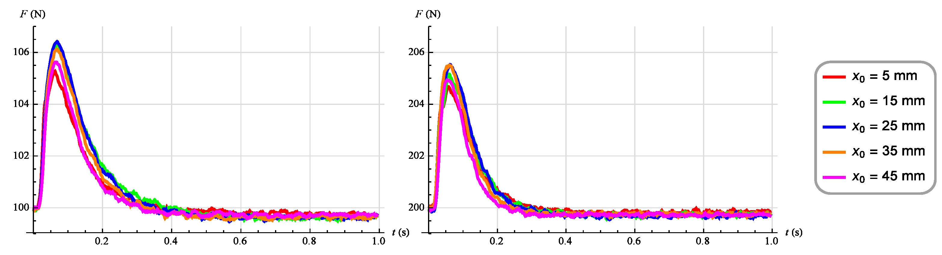
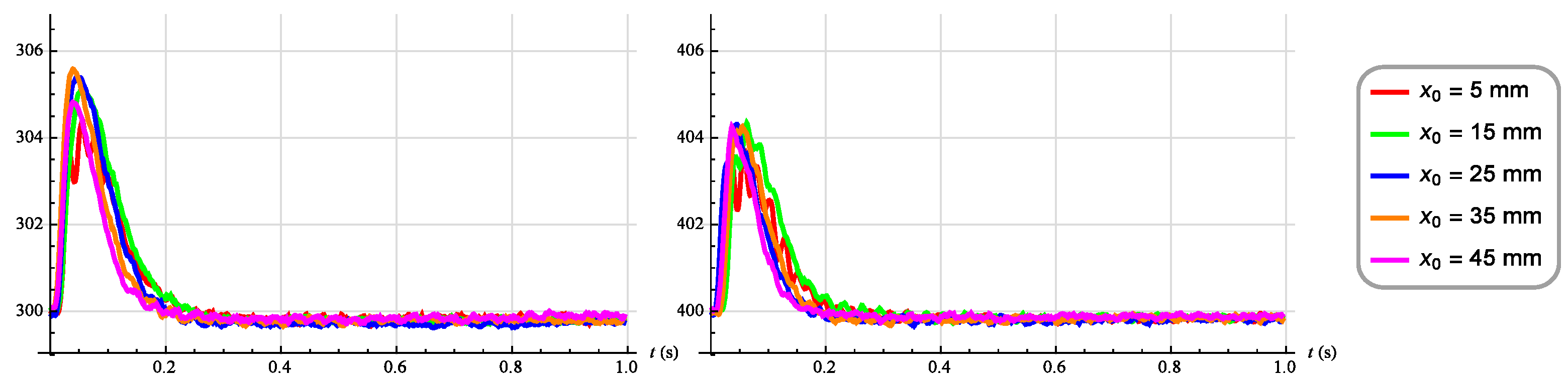
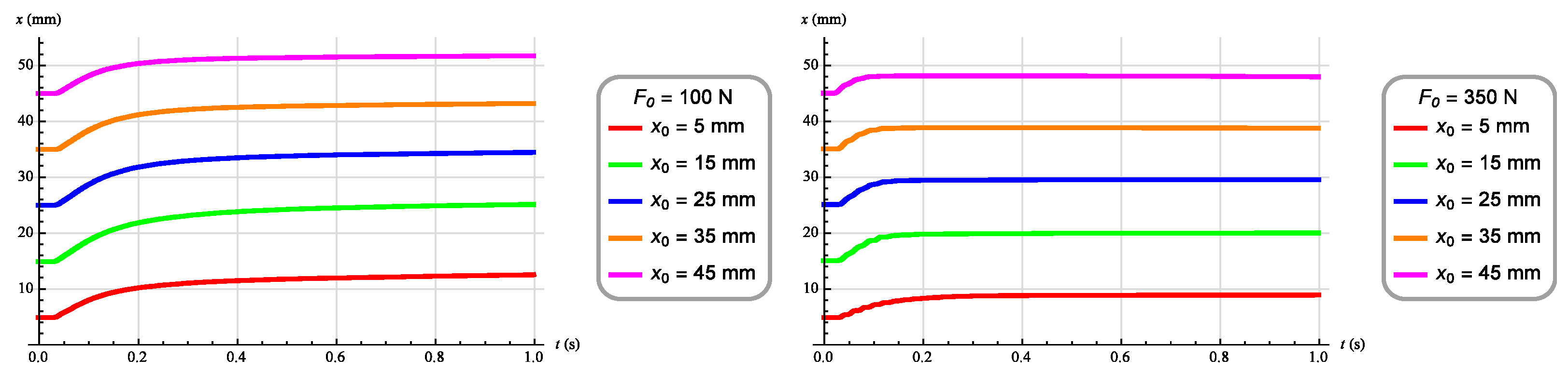
2.3. Dynamic Characteristics

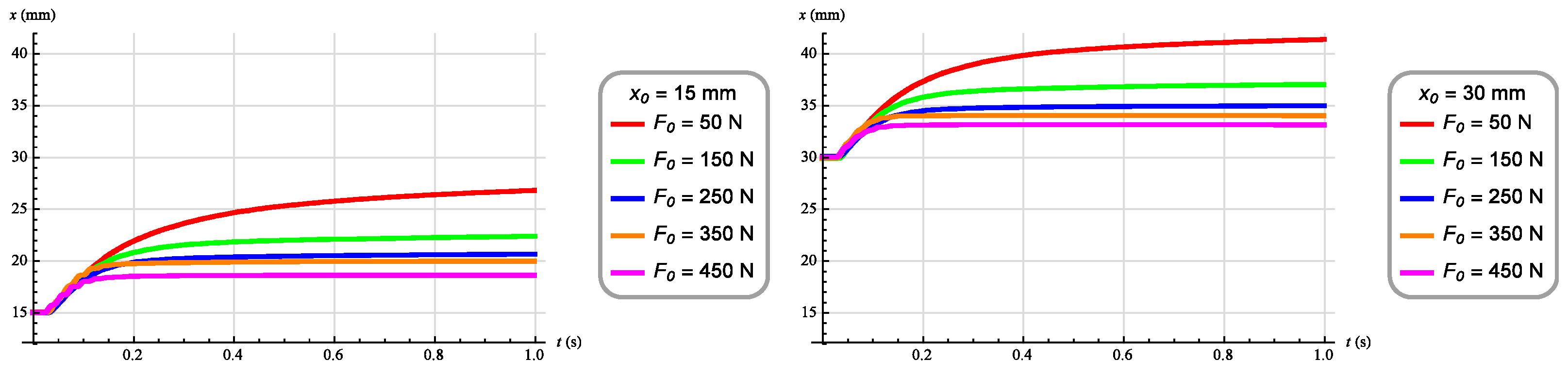
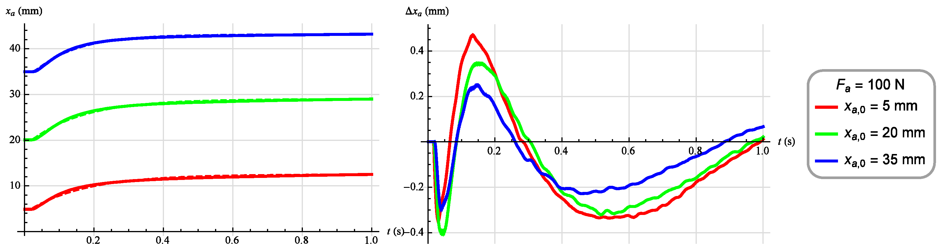
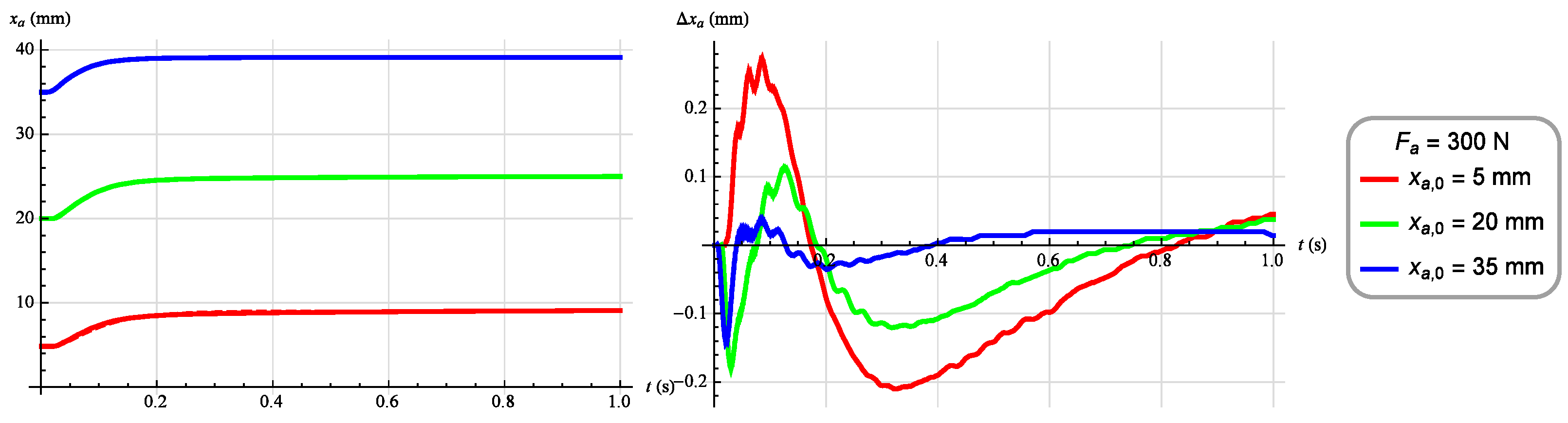
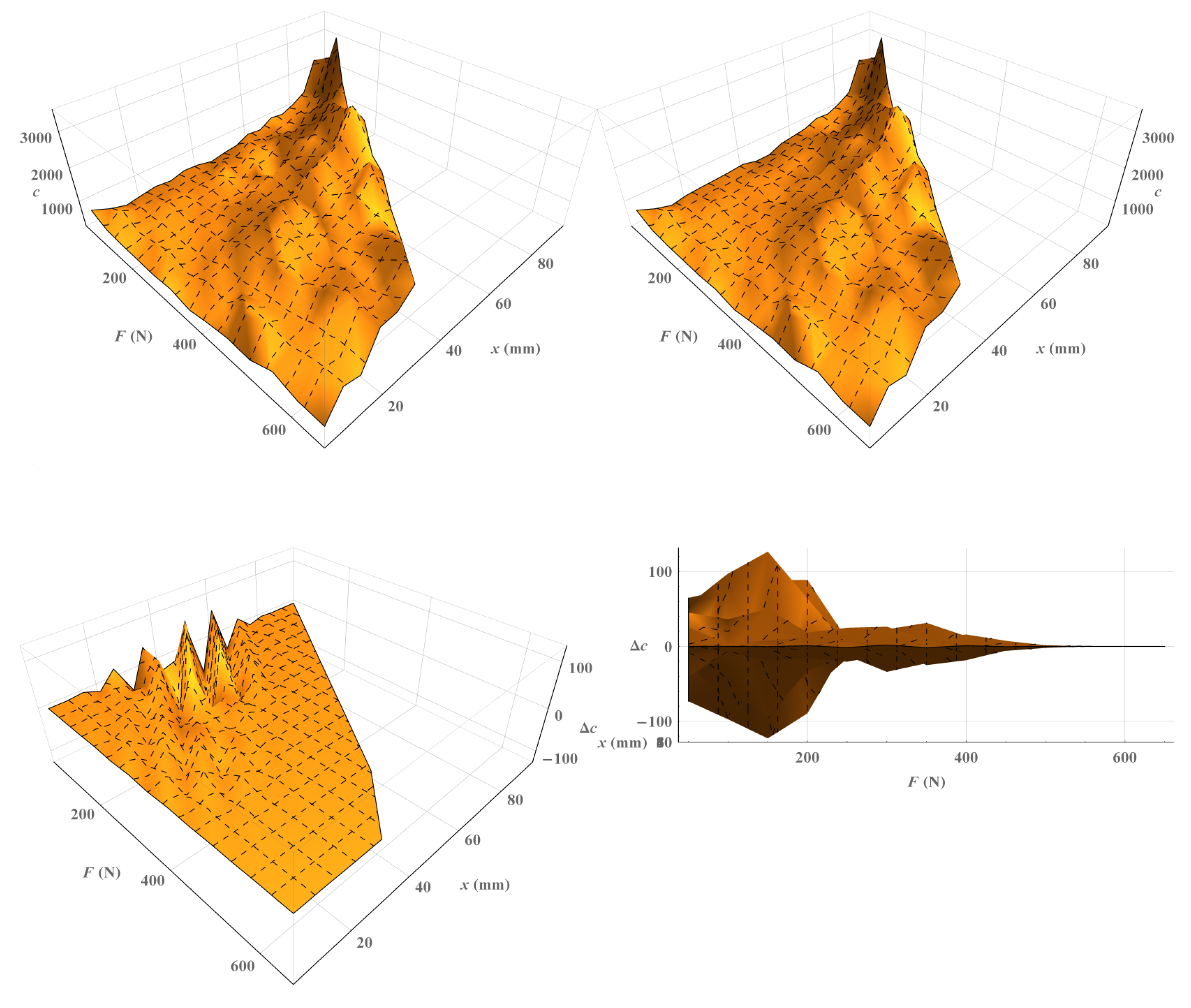
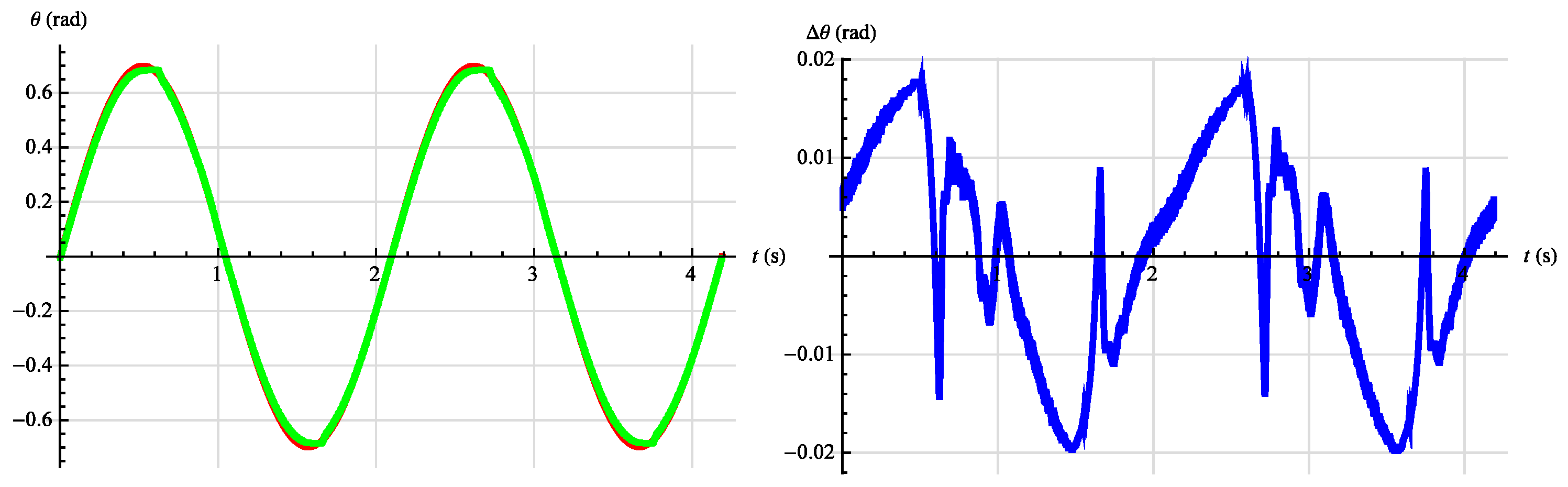
In the first stage, a set of characteristics was determined for showing the relationship between the muscle position x and time t as a response to a step change in the control signal u and with a constant value of the load force F on the muscle. A constant load force was ensured using the built-in electric servo drive with a tensometric force sensor and a PID controller. The sampling frequency in the system was 1 kHz, while the sampling frequency in the force control system was 10 kHz. The force control system provided satisfactory regulation quality for step changes in the control signal not exceeding 0.5 V. Figure 7 and Figure 8 depict the actual force values that the control system achieved for several nominal force values F and several operating points $x_{a0}$. The maximum error ranged from 4 N to 5 N.

During the determination of the dynamic characteristic, the operating point of the object was defined using the values of two output quantities: the force generated by the muscle $F_0$ and the muscle position $x_0$. Thirteen constant load force values were adopted. A set of initial muscle position values was also adopted, with the full range of positions being available only for a load force of 50 N. For higher load forces, the muscle was unable to achieve all position values, which could be anticipated by analyzing the static characteristics of the object. For the maximum load force value of $F_0=650$ N, the maximum initial muscle position was $F_0=35$ mm. Therefore, for each operating point, one dynamic characteristic was determined by applying a control signal to the valve with a stepwise-varying value from $u_0$ to $u_n=u_0+0.2$ V, where $u_0$ was chosen so that the muscle would assume the desired position value $x_0$ for that operating point. The muscle position was measured for a period of 1 s at a sampling frequency of 1 kHz. Figure 9 and Figure 10 depict the dynamic characteristics for several selected operating points of the object.

The determined dynamic characteristics were analyzed. These characteristics took the form of a change in the position of the muscle in response to a step change in the control signal at a constant loading force, as depicted in Figure 9 and Figure 10. It was noticed that the behavior of the tested object in the vicinity of a given operating point corresponds to the behavior of a second-order object of an inertial or slightly oscillatory nature.

3. Results

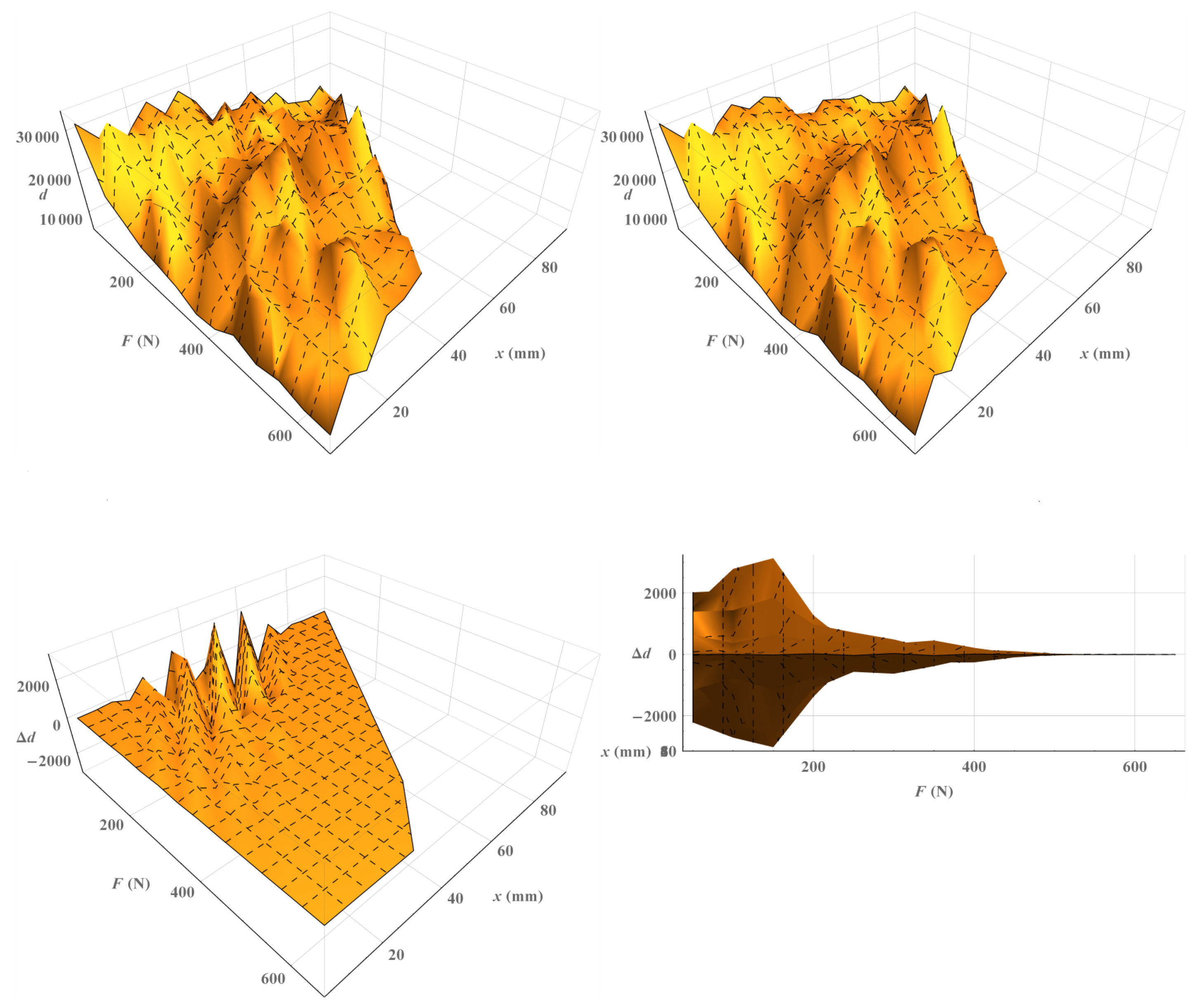
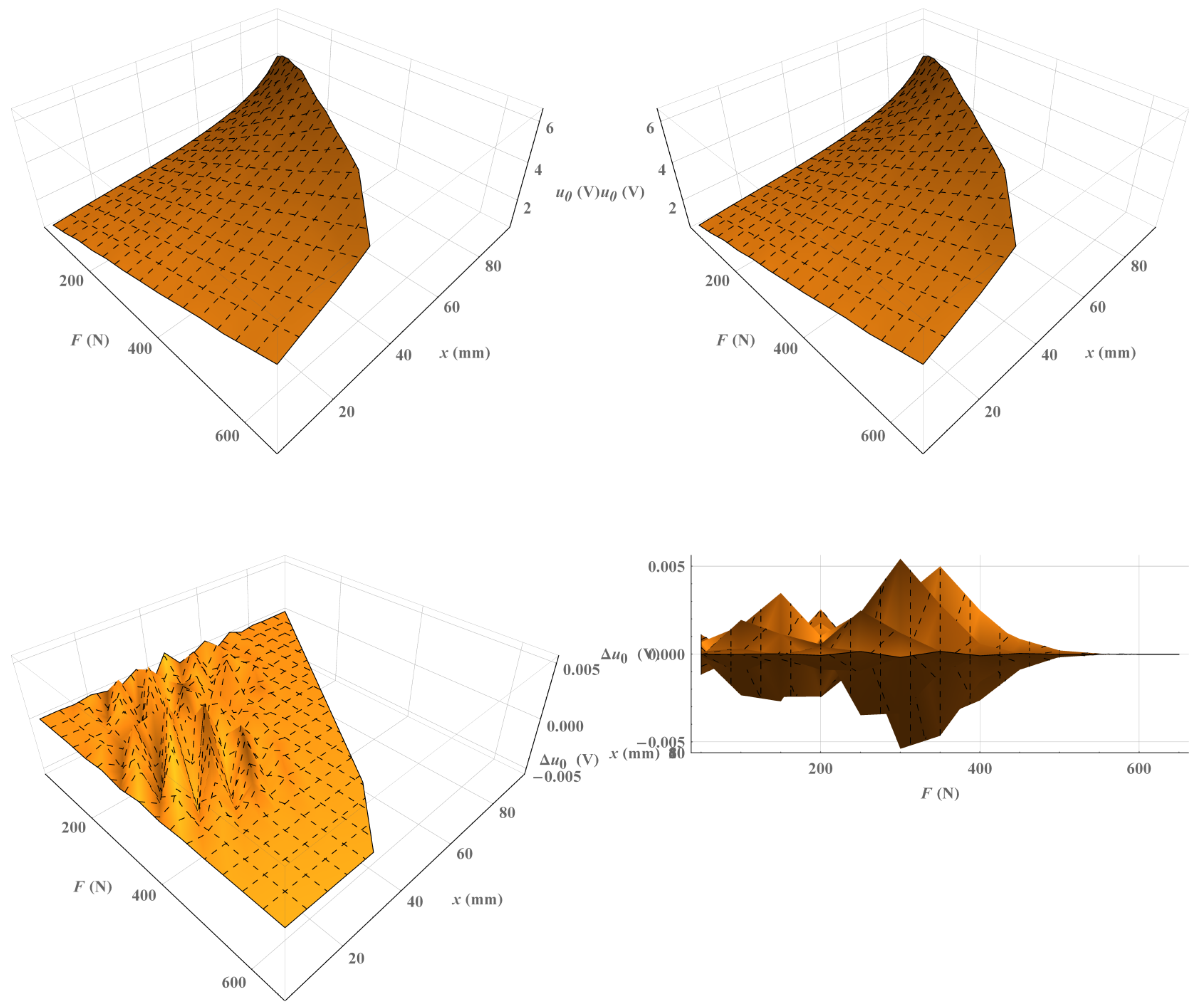
3.1. Functional Model of the Pneumatic Muscle

Analyzing the static characteristics of the muscle, it was observed that the static relationship between the muscle position x and the control signal u is highly nonlinear. However, the relationship between the force generated by the muscle F and the control signal u can be approximated as linear within the full range of muscle positions x. Analyzing the dynamic characteristics determined in Section 2.3, it was noticed that the behavior of the object around a given operating point can be approximately described by a second-order differential equation with constant coefficients and with initial conditions as presented in Equation (1).

$$\begin{array}{c}\ddot{x}+b\dot{x}+cx=du\hfill \\ x(0)=x_{a,0},\dot{x}(0)=0,u(0)=u_{a,0}(F_a,x_{a,0})\hfill \end{array}$$

(1)

where x represents the muscle position expressed in coordinates relative to the operating point, u denotes the control signal expressed in coordinates relative to the operating point, and b, c, and d are the constant coefficients of the equation. The operating point, on the other hand, was determined in absolute coordinates by the relationship $u_{a,0}=g(F_a,x_{a,0})$ by using parameters such as the load force on the muscle $F_a$, which was maintained at a constant level throughout the study, and the initial muscle position $x_{a,0}$, which corresponds directly to the initial control signal value $u_{a,0}$. Then, utilizing Wolfram Mathematica software version 13.3.1, the responses to step inputs obtained in Section 2.3 for individual operating points were fitted to the solution of Equation (1) and are presented as Equation (2).

$$\begin{array}{cc}x(t)\hfill & =\frac{1}{2\sqrt{b^2-4c}c}{e}^{-\frac{1}{2}(b+\sqrt{b^2-4c})t}(-b(-1+e^{\sqrt{b^2-4c}t})(du+u_{a,0}(F_a,x_{a,0})-c{x}_{a,0})\hfill \\ \hfill & +\sqrt{b^2-4c}(d(-1+2e^{\frac{1}{2}(b+\sqrt{b^2-4c})t}-e^{\sqrt{b^2-4c}t})u)\hfill \\ \hfill & +(-1+2e^{\frac{1}{2}(b+\sqrt{b^2-4c})t}-e^{\sqrt{b^2-4c}t})u_{a,0}(F_a,x_{a,0})+c(1+e^{\sqrt{b^2-4c}t})x_{a,0})\hfill \end{array}$$

(2)

The results of this fitting for several selected step responses are presented below. In Figure 11 and Figure 12, the real object responses to step inputs are shown with solid lines on the left side, while the responses of the fitted model are represented with dashed lines. In Figure 11 and Figure 12 on the right side, the absolute fitting error for each response is depicted.

As a result, for each response of the object, and thus, for each operating point determined by the parameters $F_a,x_{a,0}$, values of the coefficients $b,c,d,u_{a,0}$ of Equation (2) were obtained. The values of these coefficients at selected operating points are presented in

Table 1. The coefficient values for operating points at $F_a=100$ N.

${\mathit{x}}_{\mathit{a},0}$ (mm)	b	c	d	${\mathit{u}}_{\mathit{a},0}$ (V)
5	122.62	957.41	33,330.0	0.84
10	112.76	775.59	31,335.3	0.95
15	94.08	662.68	31,716,3	1.06
20	69.14	524.55	21,838.9	1.12
25	73.56	577.66	25,709.5	1.22
30	67.61	560.13	23,357.6	1.31
35	72.27	624.12	24,316.4	1.40
40	64.26	576.44	20,535.6	1.51
45	77.82	750.06	24,096.8	1.63
50	65.02	654.24	18,675.3	1,76
55	81.97	887.24	21,933.3	1.92
60	69.79	793.37	17,452.7	2.10
65	62.50	748.39	13,045.2	2.30
70	66.51	848.06	12,567.3	2.58
75	71.27	1056.75	13,055.3	2.90
80	68.15	1089.00	10,214.1	3.32
85	88.18	1539.92	10,914.0	3.89
90	122.07	2545.10	13,172.4	4.69

,

Table 2. The coefficient values for operating points at $F_a=200$ N.

${\mathit{x}}_{\mathit{a},0}$ (mm)	b	c	d	${\mathit{u}}_{\mathit{a},0}$ (V)
5	97.61	953.89	25,126.8	1.42
10	79.22	742.11	24,444.6	1.58
15	68.20	682.04	19,716.6	1.68
20	57.16	573.95	17,407.9	1.82
25	62.43	665.15	19,953.9	1.97
30	64.07	752.55	21,483.4	2.11
35	58.90	708.48	19,054.1	2.27
40	57.11	725.15	17,903.7	2.44
45	72.61	982.46	21,409.4	2.64
50	44.88	576.91	10,872.4	2.86
55	61.77	935.85	15,833.9	3.12
60	82.39	1387.44	19,843.6	3.42
65	94.31	1712.43	20,007.5	3.78
70	81.78	1636.40	15,931.9	4.23
75	91.88	2123.36	16,771.0	4.79
80	103.93	2570.42	15,668.4	5.54

,

Table 3. The coefficient values for operating points at $F_a=300$ N.

${\mathit{x}}_{\mathit{a},0}$ (mm)	b	c	d	${\mathit{u}}_{\mathit{a},0}$ (V)
5	87.87	1071.91	21,538.4	2.00
10	60.36	690.15	15,207.9	2.20
15	60.37	732.23	18,077.5	2.38
20	61.67	794.31	19,306.4	2.55
25	64.50	908.30	21,698.3	2.74
30	71.17	1065.53	23,788.4	2.94
35	70.42	1138.32	23,425.3	3.15
40	69.60	1095.38	19,684.4	3.40
45	67.53	1187.75	19,249.2	3.67
50	73.07	1319.48	18,167.5	3.99
55	87.03	1695.44	19,666.4	4.36
60	78.60	1748.91	17,782.4	4.79
65	110.72	2804.38	23,168.6	5.33
70	90.49	2365.22	16,692.0	6.01

and

Table 4. The coefficient values for operating points at $F_a=400$ N.

${\mathit{x}}_{\mathit{a},0}$ (mm)	b	c	d	${\mathit{u}}_{\mathit{a},0}$ (V)
5	83.92	1079.55	16,687.1	2.58
10	67.30	835.22	13,068.6	2.81
15	75.73	1002.05	18,387.3	3.05
20	80.71	1174.23	21,503.9	3.28
25	77.49	1350.28	20,937.3	3.48
30	84.94	1613.87	27,991.7	3.78
35	70.51	1229.30	18,264.0	4.06
40	78.05	1549.41	21,158.5	4.39
45	87.73	1861.74	22,103.3	4.75
50	80.10	1918.73	19,903.4	5.17
55	75.60	1853.75	17,117.1	5.68
60	86.73	2307.93	18,940.3	6.29

.

For each coefficient, a two-dimensional array of values was created: one for each step response. The position in the array depends on the operating point for which the coefficient was determined. Then, the arrays of values for each coefficient were approximated using a two-variable polynomial according to Equation (3).

$$w(F,x)=a_{ij}{x}^i{F}^j$$

(3)

In Figure 13, Figure 14, Figure 15 and Figure 16, the top left side shows surfaces created from the real values of the coefficients, while the top right side displays surfaces resulting from the approximation. The bottom part illustrates surfaces representing the absolute approximation error.

Next, the obtained polynomials were inserted into Equations (1) and (2), resulting in a model describing the behavior of the object in the form of a second-order differential equation solution, described by Equation (4). Additionally, an inverse model was obtained in the form of a second-order differential equation, described by Equation (5). The model has coefficients that are two-variable polynomials defining the operating point of the object.

$$\begin{array}{cc}\hfill (x(t)& =\frac{1}{2\sqrt{b{(F_a,x_a)}^2-4c(F_a,x_a)}}c(F_a,x_a)e^{-\frac{1}{2}(b(F_a,x_a)+\sqrt{b{(F_a,x_a)}^2-4c(F_a,x_a)})t}\hfill \\ \hfill & (-b(F_a,x_a)(-1+e^{\sqrt{b{(F_a,x_a)}^2-4c(F_a,x_a)}t})(d(F_a,x_a)u+u_a-c(F_a,x_a)(F_a,x_a))\hfill \\ \hfill & +\sqrt{b{(F_a,x_a)}^2-4c(F_a,x_a)}(d(F_a,x_a)\hfill \\ \hfill & (-1+2e^{\frac{1}{2}(b(F_a,x_a)+\sqrt{b{(F_a,x_a)}^2-4c(F_a,x_a)}}t)e^{\sqrt{b{(F_a,x_a)}^2-4c(F_a,x_a)}t})u\hfill \\ \hfill & +(-1+2e^{\frac{1}{2}(b(F_a,x_a)+\sqrt{b{(F_a,x_a)}^2-4c(F_a,x_a)})t})e^{\sqrt{b{(F_a,x_a)}^2-4c(F_a,x_a)}t}{u}_a\hfill \\ \hfill & +c(F_a,x_a)(1+e^{\sqrt{b{(F_a,x_a)}^2-4c(F_a,x_a)}t})(F_a,x_a)))\hfill \end{array}$$

(4)

$$\ddot{x}+b(F_a,x_a)\dot{x}+c(F_a,x_a)x=d(F_a,x_a)u+u_a(F_a,x_a)$$

(5)

Since the inverse model presented was developed for use in the control system synthesis for the servo drive used in the parallel manipulator, it can be expected that in most cases, the reference signals for the servo drive will have waveforms close to sinusoidal with relatively low frequencies. Therefore, it is possible that for such slowly varying reference signals, satisfactory results could be obtained using a static inverse model. As observed, in the developed dynamic inverse model (Equation (5)), the static part is represented by the term $u_a(F_a,x_a)$. Since developing a dynamic inverse model requires significantly more effort than a static one, a decision was made to verify both dependencies and make a quantitative comparison between them. To achieve this, both models were used to control the object in an open-loop configuration. The control system setup used for verification is depicted in Figure 17.

The dynamic inverse model requires information about the current operating point of the object. For this purpose, the model was provided with the muscle position value $x_a$ and the muscle load force value $F_a$. The desired position value that the muscle should achieve $x_{a,zad}$ was also input into the inverse model. These values are expressed in absolute coordinates and are used to calculate the desired muscle position x in terms of deflection coordinates. Based on the input data, the model generates the control voltage $u_a=u+u_{a,0}$, which is then applied to the control valve. Similarly, the static inverse model requires the current load force $F_a$ and the desired position value for the muscle to achieve $x_{a,zad}$. The result of the static inverse model’s operation is also the generation of the control voltage applied to the valve.

In Figure 18 and Figure 19, the results of the verification of both developed inverse models are presented. On the left side, the desired position value that the muscle was supposed to achieve is marked in red, the measured muscle position value when controlling the static model is marked in green, and the measured position value when controlling the dynamic model is marked in blue. On the right side, the control errors using both models are shown.

In

Table 5. Results of comparison between the dynamic model and the static model.

	Static Model (mm)	Dynamic Model (mm)
$x_{a,zad}=15sin(5t)+20$ mm $F_a=250$ N	2.21	1.71
$x_{a,zad}=15sin(3t)+35$ mm $F_a=350$ N	1.14	0.60

, the results of the quantitative comparison of the performance of both mathematical models are presented in terms of the average absolute error. These indicators were calculated in the time interval from the beginning of the second to the end of the third period of the reference sinusoidal signal. This time interval was chosen to make the comparison independent of the initial phase of the drive motion.

Analyzing the results of the operation of both mathematical models—static and dynamic, presented in Figure 18 and Figure 19—it was found that they reflect the behavior of the object in a way that meets the authors’ expectations. It can be presumed that each of them can be successfully used to build a servo drive for a parallel manipulator. However, a direct comparison of both models, based on the values presented in Table 5, indicates that the dynamic model provides a significantly smaller value of the examined quality indicator. Therefore, despite the fact that developing the dynamic model requires much more effort than developing the static model, it was chosen as the basis for the operation of the angular position servo drive discussed in Section 3.2.

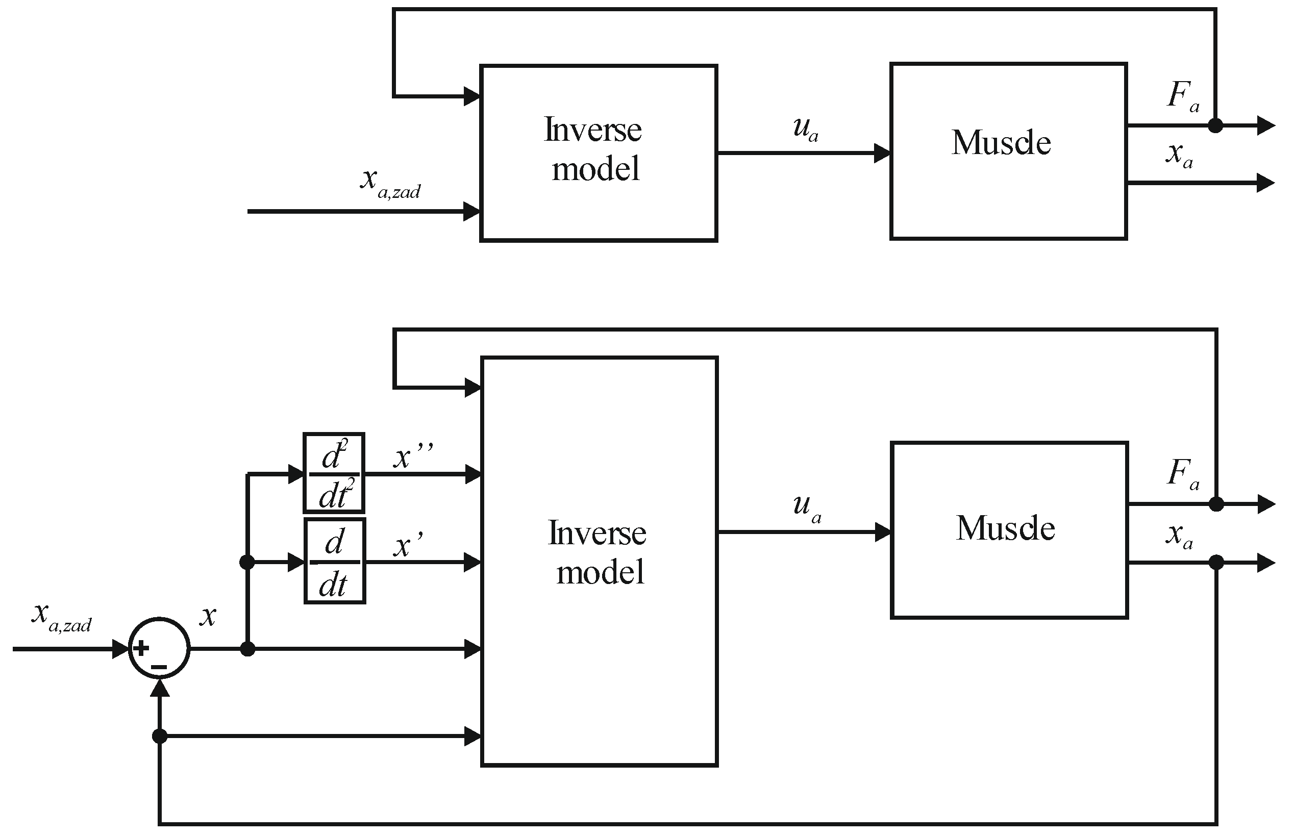
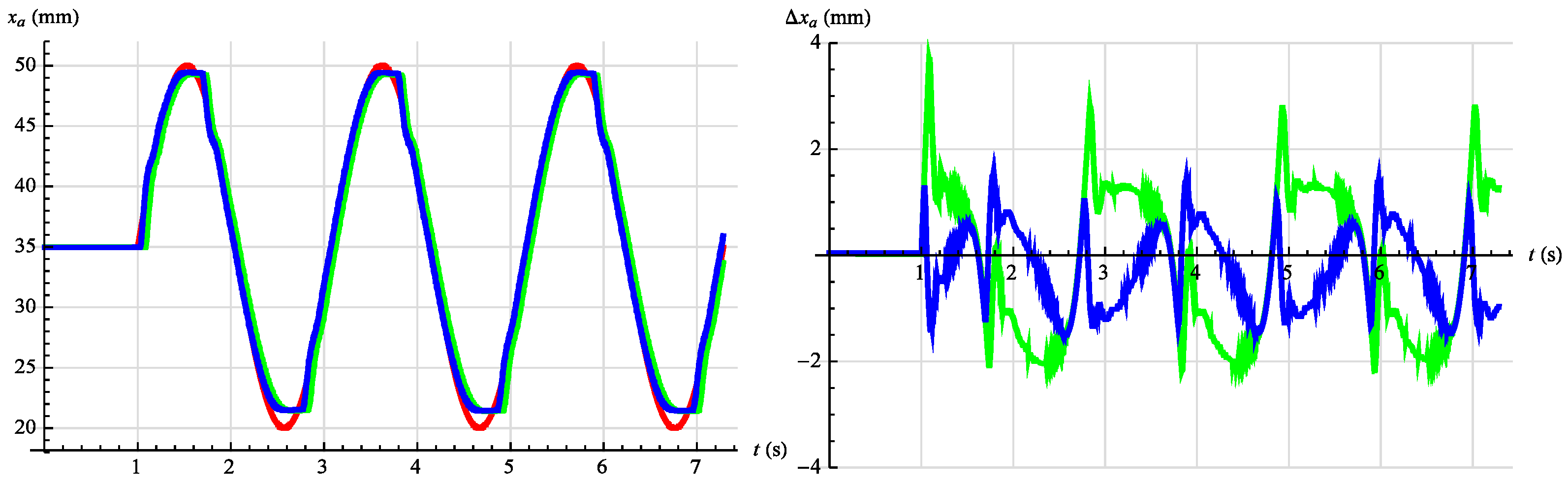
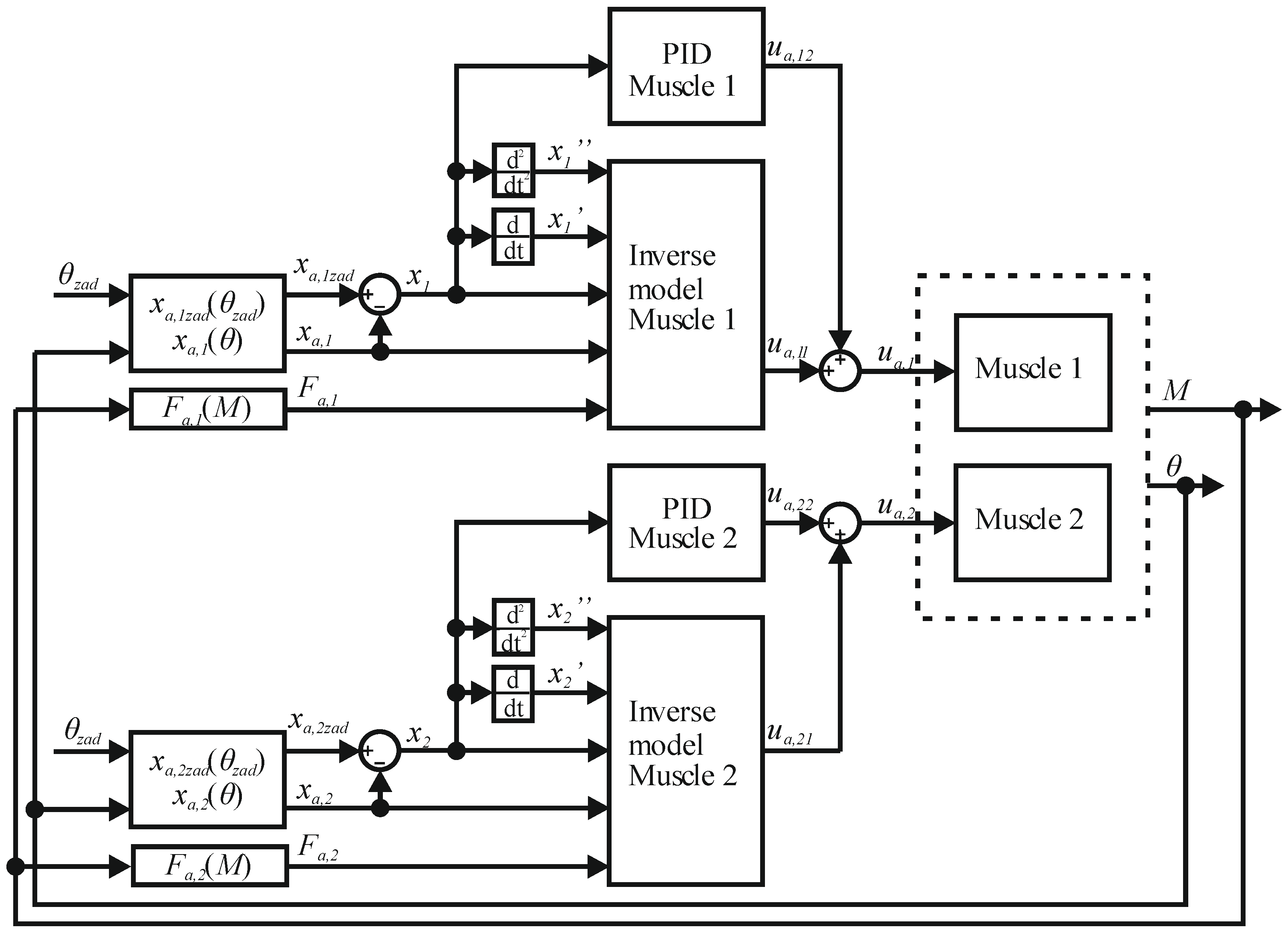
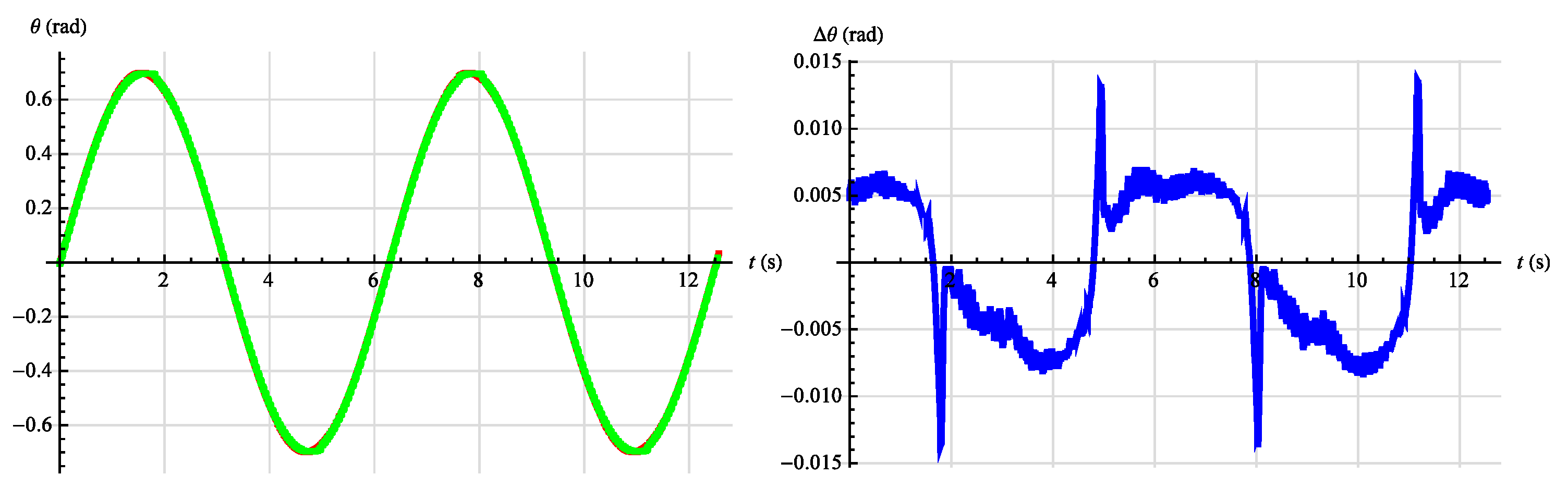
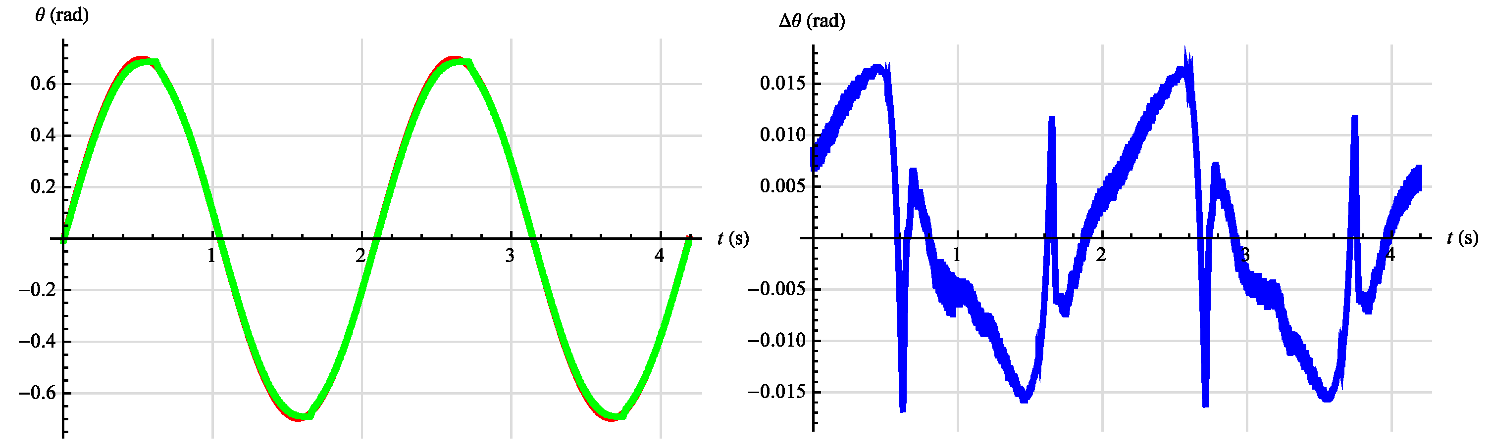
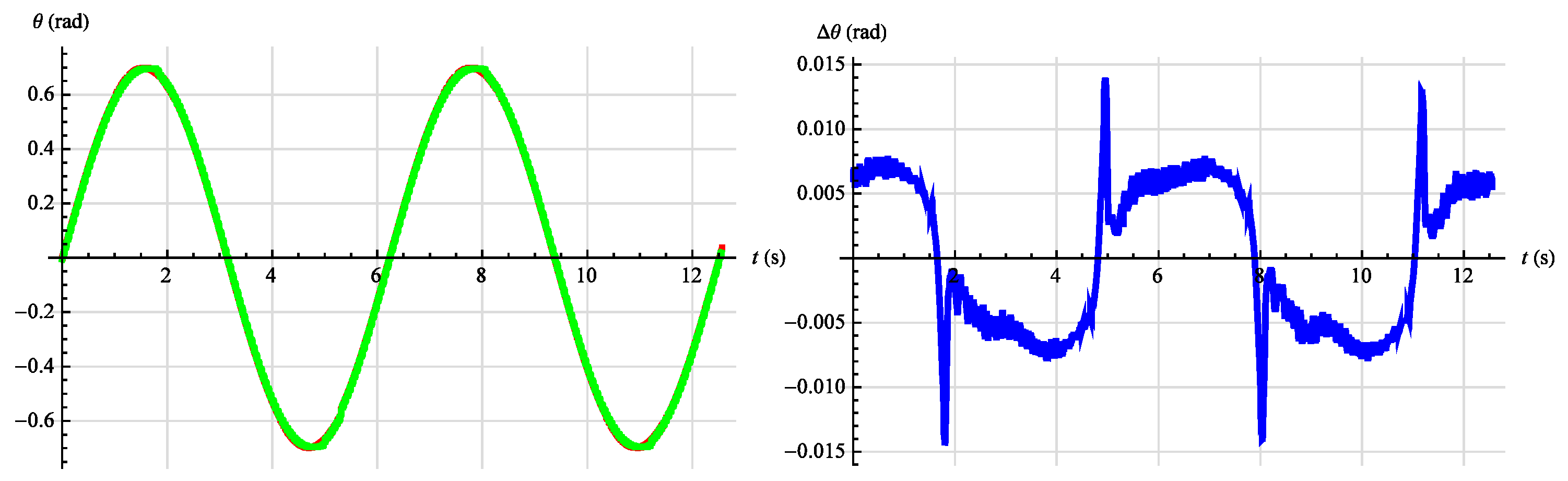
3.2. Synthesis of Angular Position Control System

The servo drive presented in this chapter is used to achieve the desired angular position for a single arm of a parallel manipulator. Its schematic, with the locations of all components marked, is shown in Figure 20.

It consists of two pneumatic muscles (4). In each of them, one end is immobilized by connecting it to the stationary base (7) through a force-sensing load cell (6) with a range of ±2 kN. The free ends of the muscles are connected together by a toothed belt (2) driving a gear wheel with a pitch diameter of $d_p=63.66$ mm, thus forming a toothed belt transmission through which the antagonistic action of the muscles is converted into the rotational motion of the arm. The pitch diameter of the pulley and the length of the muscles allow the servo drive to move in the range of $-\frac{pi}{3}$ rad to $\frac{pi}{3}$ rad, and the maximum force generated by a single muscle allows for the generation of a torque equal to $M=25.46$ Nm. The servo drive is also equipped with two pneumatic pressure-control servo valves (5) that control the operation of the muscles and an absolute angular position sensor (1) with a resolution of 16 bits per revolution, allowing the measurement of angular position with an accuracy of 0.000096 rad. The diagram also shows an electric servo drive (3), which was used in the research setup to load the muscle servo drive with a specified torque.

Then, the synthesis of the control system for the angular position servo drive was carried out. Figure 21 shows the control system diagram for the entire servo drive.

The servo drive control system consists of two independently operating control systems, one for each muscle, in which the controlled variables are the linear positions of the muscles. The desired angular position signal of the servo drive is converted into a desired linear position of the first muscle and input into the inverse model of the first muscle. Similarly, the current angular position signal of the servo drive is converted into the current linear position value of the first muscle and input into its inverse model. The current force signal generated by the muscle, which comes from the strain gauge force sensor CL21msrs produced by ZEPWN (Marki, Poland), is also input into this model. Then, the control signal is determined based on the inverse model of the first muscle. Any discrepancies between the setpoint and the actual linear position value of the first muscle, resulting from inaccuracies in the model, are compensated for by a PID controller. The signal generated by the controller is added to the signal generated by the inverse model, and the sum of the signals is converted into a control voltage for the valve of the first muscle using a digital-to-analog converter. The PID controller parameters were adjusted during tests of the servo drive on the test bench. A similar operating principle is applied to the control system of the second muscle.

In Figure 22, Figure 23, Figure 24, Figure 25 and Figure 26, the results of the tests conducted on the developed servo drive maintaining the desired angular position are presented. The left graph shows the course of the setpoint and actual values, while the right graph shows the absolute error of the servo drive operation. The setpoint signal is represented in red, the measured value is in green, and the error is in blue.

Table 6. Results of angular position servo drive operation.

	${\mathit{e}}_{\mathbf{mean}}$ (rad)	${\mathit{e}}_{\mathbf{max}}$ (rad)
$thet{a}_{zad}=\frac{2pi}{9}sin(t)$ rad $M=0$ Nm	0.0051	0.013
$thet{a}_{zad}=\frac{2pi}{9}sin(3t)$ rad $M=0$ Nm	0.008	0.016
$thet{a}_{zad}=\frac{2pi}{9}sin(t)$ rad $M=5$ Nm	0.005	0.013
$thet{a}_{zad}=\frac{2pi}{9}sin(3t)$ rad $M=5$ Nm	0.009	0.018
$thet{a}_{zad}=step$ rad $M=0$ Nm	0.028	1.047

presents the results of the evaluation of the performance of the developed servo drive. For all four sinusoidal waveforms and one square waveform, the average absolute error and the maximum absolute error were calculated. All parameters were calculated over a time interval covering two complete cycles of the reference signal, starting from the second complete cycle.

Analyzing the results of the tests conducted on the developed angular position servo drive, it was observed that in the case of sinusoidal signals, the largest error occurs when changing the direction of motion of the drive. This is likely due to the presence of friction forces between the muscle bundle fibers and between the fibers and the rubber bladder. The influence of friction forces on positioning accuracy is most significant at muscle velocities close to zero. It was also noticed that for low-frequency signals, apart from the moment of changing the direction of the drive, the error value changes slightly and is not dependent on the current drive position. However, a strong correlation between the external load and the positioning accuracy of the servo drive was not observed. This is evidenced by the fact that the average absolute error values, as presented in Table 6, for signals with the same pulsations are close to each other. Similarly, the average absolute error values for signals with the same pulsations do not differ significantly from each other. Analyzing the test results, it was observed that the maximum average absolute error value for sinusoidal signals is 0.028 radians, which translates to a muscle positioning error of 0.89 mm considering the pitch diameter of the belt drive. Analyzing the static characteristics of the muscle and considering the high static gain of the system, it was noted that, depending on the operating point of the system, a 0.015 V change in the control signal corresponds to 0.89 mm of positioning error. The manufacturer guarantees a precision of 0.1% for the operation of the servo valves, which corresponds to a value of 0.01 V within the control signal range. Taking into account the above considerations, it was concluded that achieving better positioning accuracy may be very difficult or impossible.

4. Conclusions

This article contains the results of research aimed at developing a pneumatic servo drive composed of two pneumatic muscles. This servo drive is being developed to be used to drive a parallel manipulator with six degrees of freedom.

The article presents a comparison of the authors’ original muscle with the commercial muscle. Both solutions have unique features. Each of them has advantages and disadvantages, which means that both can be successfully used to drive manipulators. Comparing them in full is very difficult because they are completely different products. However, by analyzing the results of an unbiased comparison, it can be noticed that the authors’ original muscle is characterized by greater strength and greater relative shortening. At the same time, it should be assumed that commercial muscles will be much more durable and resistant to damage. However, considering the very low cost of making the authors’ original muscle, it should be assumed that replacing it more often will not be a big problem.

This article presents a mathematical model of the authors’ muscle. This is a functional model. It was determined through a series of many experiments: mostly step responses. The procedure for its development makes this task time-consuming and labor-intensive. The lack of a structural model means that this procedure must be repeated for each muscle separately. This may be considered a disadvantage of this solution. In a 6-DoF manipulator, 12 muscles need to be used. However, as will be presented in the next publication, even the authors’ muscles performed in a repeatable manner. Thanks to this, the parameters of the mathematical models of individual muscles do not differ significantly. It is sufficient to perform parameterization for several muscles (for example, four) and average the results. Moreover, to further simplify and shorten the identification stage, a test stand was developed to automate the entire process. This significantly reduced the time needed for identification.

The article also presents the synthesis of a servo drive consisting of two pneumatic muscles. The use of the developed mathematical models (in the form of inverse models) in the control process significantly eliminated the non-linearities of muscle work. This approach allowed us to get rid of the influence of the non-linearity of the static characteristics of the object. This made it possible to use a PID controller with constant coefficients. However, other non-linearities, especially those resulting from the friction of the braid and rubber bladder, still negatively affect the operation of the drive. This is especially visible at low operating speeds. This is one of the main limitations of the adopted servo drive synthesis method and will be one of the most important topics of further research.

Based on the analysis of the presented results and the conclusions drawn, the decision was made to justify the use of the developed servo drive for the construction of a delta-type parallel manipulator with six degrees of freedom. The manipulator, mentioned several times in this article, will be presented in subsequent work.

References

1. Pietrala, D.S.; Łaski, P.A. Design and Control of a Pneumatic Muscle Servo Drive Containing Its Own Pneumatic Muscles. Appl. Sci. 2022, 12, 11024. [Google Scholar] [CrossRef]
2. Nazarczuk, K. Niektóre Zagadnienia Analizy i Syntezy Sztucznego Mięśnia Pneumatycznego; Archiwum Budowy Maszyn: Warszawa, Poland, 1967. [Google Scholar]
3. Chou, C.P.; Hannaford, B. Static and Dynamic Characteristics of McKibben Pneumatic Artificial Muscles. In Proceedings of the 1994 IEEE International Conference on Robotics and Automation, San Diego, CA, USA, 8–13 May 1994; Volume 1–4, pp. 281–286. [Google Scholar]
4. Chou, C.P.; Hannaford, B. Measurement and modeling of McKibben pneumatic artificial muscles. IEEE Trans. Robot. Autom. 1996, 12, 90–102. [Google Scholar] [CrossRef]
5. Doumit, M.; Fahim, A.; Munro, M. Analytical Modeling and Experimental Validation of the Braided Pneumatic Muscle. IEEE Trans. Robot. 2009, 25, 1282–1291. [Google Scholar] [CrossRef]
6. Takosoglu, J.E.; Łaski, P.A.; Blasiak, S.; Bracha, G.; Pietrala, D. Determining the Static Characteristics of Pneumatic Muscles. Meas. Control 2016, 49, 62–71. [Google Scholar] [CrossRef]
7. Tondu, B.; Lopez, B. Modeling and control of McKibben artificial muscle robot actuators. IEEE Control. Syst. Mag. 2000, 20, 15–38. [Google Scholar]
8. Pietrala, D. The characteristics of a pneumatic muscle. EPJ Web Conf. 2017, 143, 02093. [Google Scholar] [CrossRef]
9. Pietrala, D.S. Analiza i Synteza Pneumatycznego Serwonapędu Mięśniowego w Zastosowaniu do Manipulatora Równoległego o Sześciu Stopniach Swobody. Ph.D. Thesis, Politechnika Świętokrzyska, Kielce, Poland, 2020. [Google Scholar]
10. Carvalho, A.D.D.R.; Karanth, P.N.; Desai, V. Characterization of pneumatic muscle actuators and their implementation on an elbow exoskeleton with a novel hinge design. Sens. Actuators Rep. 2022, 4, 100109. [Google Scholar] [CrossRef]
11. Dyrr, F.; Dvorak, L.; Fojtasek, K.; Brzezina, P.; Hruzik, L.; Burecek, A. Experimental analysis of fluidic muscles. MM Sci. J. 2022, 2022, 5759–5763. [Google Scholar] [CrossRef]
12. Xavier, M.S.; Tawk, C.D.; Zolfagharian, A.; Pinskier, J.; Howard, D.; Young, T.; Lai, J.; Harrison, S.M.; Yong, Y.K.; Bodaghi, M.; et al. Soft Pneumatic Actuators: A Review of Design, Fabrication, Modeling, Sensing, Control and Applications. IEEE Access 2022, 10, 59442–59485. [Google Scholar] [CrossRef]
13. Kalita, B.; Leonessa, A.; Dwivedy, S.K. A Review on the Development of Pneumatic Artificial Muscle Actuators: Force Model and Application. Actuators 2022, 11, 288. [Google Scholar] [CrossRef]
14. Ganguly, S.; Garg, A.; Pasricha, A.; Dwivedy, S.K. Control of pneumatic artificial muscle system through experimental modelling. Mechatronics 2012, 22, 1135–1147. [Google Scholar] [CrossRef]
15. Godage, I.S.; Branson, D.T.; Guglielmino, E.; Caldwell, D.G. Pneumatic Muscle Actuated Continuum Arms: Modelling and Experimental Assessment. In Proceedings of the 2012 IEEE International Conference on Robotics and Automation (ICRA), Saint Paul, MN, USA, 14–18 May 2012; pp. 4980–4985. [Google Scholar]
16. Kang, B.-S.; Kothera, C.S.; Woods, B.K.S.; Wereley, N.M. Dynamic Modeling of McKibben Pneumatic Artificial Muscles for Antagonistic Actuation. In Proceedings of the ICRA 2009 IEEE International Conference on Robotics and Automation, Kobe, Japan, 17 May 2009; Volume 1–7, p. 643. [Google Scholar]
17. Shen, X. Nonlinear model-based control of pneumatic artificial muscle servo systems. Control Eng. Pract. 2010, 18, 311–317. [Google Scholar] [CrossRef]
18. Zhang, D.; Zhao, X.; Han, J. Active Model-Based Control for Pneumatic Artificial Muscle. IEEE Trans. Ind. Electron. 2017, 64, 1686–1695. [Google Scholar] [CrossRef]
19. Dai, Z.; Rao, J.; Xu, Z.; Lei, J. Design and Joint Position Control of Bionic Jumping Leg Driven by Pneumatic Artificial Muscles. Micromachines 2022, 13, 827. [Google Scholar] [CrossRef]
20. Andrikopoulos, G.; Nikolakopoulos, G.; Manesis, S. Advanced Nonlinear PID-Based Antagonistic Control for Pneumatic Muscle Actuators. IEEE Trans. Ind. Electron. 2014, 61, 6926–6937. [Google Scholar] [CrossRef]
21. Minh, T.V.; Tjahjowidodo, T.; Ramon, H.; Brussel, H.V. Control of a Pneumatic Artificial Muscle (PAM) with Model-Based Hysteresis Compensation. In Proceedings of the 2009 IEEE/ASME International Conference on Advanced Intelligent Mechatronics, Suntec Convention and Exhibition Center, Singapore, 14–17 July 2009; Volume 1–3, p. 1086. [Google Scholar]
22. Minh, T.V.; Tjahjowidodo, T.; Ramon, H.; Brussel, H.V. Cascade position control of a single pneumatic artificial muscle-mass system with hysteresis compensation. Mechatronics 2010, 20, 402–414. [Google Scholar] [CrossRef]
23. Minh, T.V.; Kamers, B.; Ramon, H.; Brussel, H.V. Modeling Torque-Angle Hysteresis in a Pneumatic Muscle Manipulator. In Proceedings of the 2010 IEEE/ASME International Conference on Advanced Intelligent Mechatronics (AIM), Montreal, QC, Canada, 6–9 July 2010. [Google Scholar]
24. Minh, T.V.; Kamers, B.; Ramon, H.; Brussel, H.V. Modeling and control of a pneumatic artificial muscle manipulator joint—Part I: Modeling of a pneumatic artificial muscle manipulator joint with accounting for creep effect. Mechatronics 2012, 22, 923–933. [Google Scholar] [CrossRef]
25. Yeh, T.-J.; Wu, M.-J.; Lu, T.-J.; Wu, F.-K.; Huang, C.-R. Control of McKibben pneumatic muscles for a power-assist, lower-limb orthosis. Mechatronics 2010, 20, 686–697. [Google Scholar] [CrossRef]
26. Qin, Y.; Zhang, H.; Wang, X.; Han, J. Active Model-Based Hysteresis Compensation and Tracking Control of Pneumatic Artificial Muscle. Sensors 2022, 22, 364. [Google Scholar] [CrossRef] [PubMed]
Figure 1. The developed pneumatic muscle.
Applsci 14 05329 g001
Figure 2. Diagram and actual view of the research setup.
Applsci 14 05329 g002
Figure 3. Selected isobaric characteristics of the compared muscles in the range from 0.1 MPa to 0.3 MPa.
Applsci 14 05329 g003
Figure 4. Selected isobaric characteristics of the compared muscles in the range from 0.4 MPa to 0.6 MPa.
Applsci 14 05329 g004
Figure 5. Selected isometric characteristics of the compared muscles in the range from 0% to 10%.
Applsci 14 05329 g005
Figure 6. Selected isometric characteristics of the compared muscles in the range from 15% to 20%.
Applsci 14 05329 g006
Figure 7. Operation of the muscle load regulation system: examples for the set force F 0 = 100 N (on the left side) and F 0 = 200 N (on the right side).
Applsci 14 05329 g007
Figure 8. Operation of the muscle load regulation system: examples for the set force F 0 = 300 N (on the left side) and F 0 = 400 N (on the right side).
Applsci 14 05329 g008
Figure 9. Dynamic characteristics of the object for selected operating points: examples for the set force F 0 = 100 N (on the left side) and F 0 = 350 N (on the right side).
Applsci 14 05329 g009
Figure 10. Dynamic characteristics of the object for selected operating points: examples for the initial position of the muscle x 0 = 15 mm (on the left side) and x 0 = 30 mm (on the right side).
Applsci 14 05329 g010
Figure 11. Results of model fitting at selected operating points of the object (on the left) and fitting error (on the right).
Applsci 14 05329 g011
Figure 12. Results of model fitting at selected operating points of the object (on the left) and fitting error (on the right).
Applsci 14 05329 g012
Figure 13. Results of the coefficient b approximation: actual surface (top left), approximation surface (top right), and approximation error (bottom).
Applsci 14 05329 g013
Figure 14. Results of the coefficient c approximation: actual surface (top left), approximation surface (top right), and approximation error (bottom).
Applsci 14 05329 g014
Figure 15. Results of the coefficient d approximation: actual surface (top left), approximation surface (top right), and approximation error (bottom).
Applsci 14 05329 g015
Figure 16. Results of the coefficient u a , 0 approximation: actual surface (top left), approximation surface (top right), and approximation error (bottom).
Applsci 14 05329 g016
Figure 17. Diagram of the muscle control system for verifying the performance of static and dynamic models.
Applsci 14 05329 g017
Figure 18. Results of verification of static and dynamic models for the given reference signal described by the equation x a , z a d = 15 s i n ( 5 t ) + 20 mm with a constant load force F a = 250 N. Left side: red—desired position, green—muscle position, blue—error. Right side: green—static model error, blue—dynamic model error.
Applsci 14 05329 g018
Figure 19. Results of verification of static and dynamic models for the given reference signal described by the equation x a , z a d = 15 s i n ( 3 t ) + 35 mm with a constant load force F a = 350 N. Left side: red—desired position, green—muscle position, blue—error. Right side: green—static model error, blue—dynamic model error.
Applsci 14 05329 g019
Figure 20. Schematic diagram of a pneumatic muscle servo drive.
Applsci 14 05329 g020
Figure 21. Control system diagram for angular position servo drive: t h e t a —current angular position of the servo drive, x a , 1 —current linear position of the first muscle, x a , 2 —current linear position of the second muscle, t h e t a z a d —desired angular position of the servo drive, x a , 1 z a d —desired linear position of the first muscle, x a , 2 z a d —desired linear position of the second muscle, M—current force moment generated by the servo drive, F a , 1 —current value of force generated by the first muscle, F a , 2 —current value of force generated by the second muscle, x 1 —regulation error for the first muscle regulator, x 2 —regulation error for the second muscle regulator, u a , 11 —component of the control signal for the first muscle valve generated by the inverse model, u a , 12 —component of the control signal for the first muscle valve generated by the PID regulator, u a , 1 —control signal for the first muscle valve, u a , 21 —component of the control signal for the second muscle valve generated by the inverse model, u a , 22 —component of the control signal for the second muscle valve generated by the PID regulator, and u a , 2 —control signal for the second muscle valve.
Applsci 14 05329 g021
Figure 22. Results of angular position servo drive operation for a reference signal described by t h e t a z a d = 2 p i 9 s i n ( t ) rad with a constant load torque M = 0 Nm: servo drive behavior (on the left side) and servo drive error (on the right side).
Applsci 14 05329 g022
Figure 23. Results of angular position servo drive operation for a reference signal described by t h e t a z a d = 2 p i 9 s i n ( 3 t ) rad with a constant load torque M = 0 Nm: servo drive behavior (on the left side) and servo drive error (on the right side).
Applsci 14 05329 g023
Figure 24. Results of angular position servo drive operation for a reference signal described by t h e t a z a d = 2 p i 9 s i n ( t ) rad with a constant load torque M = 5 Nm: servo drive behavior (on the left side) and servo drive error (on the right side).
Applsci 14 05329 g024
Figure 25. Results of angular position servo drive operation for a reference signal described by t h e t a z a d = 2 p i 9 s i n ( 3 t ) rad with a constant load torque M = 5 Nm: servo drive behavior (on the left side) and servo drive error (on the right side).
Applsci 14 05329 g025
Figure 26. Results of angular position servo drive operation for a square wave reference signal with an amplitude of A = p i 6 rad and a period of T = 6 s and with a constant load torque M = 0 : servo drive behavior (on the left side) and servo drive error (on the right side).
Applsci 14 05329 g026