Analysis of Factors Influencing Three-Dimensional Multi-Cluster Hydraulic Fracturing Considering Interlayer Effect

Abstract

This study establishes a three-dimensional cohesive model of multi-cluster hydraulic fracturing using finite element method (FEM). It fully considers the interaction between the interlayer and the reservoir and analyzes the key factors influencing fracture propagation. The results show that during the initial stage of hydraulic fracturing, the width of the edge fracture is greater than that of the mid fracture, while the situation is reversed for the fracture length. A larger cluster spacing leads to less interaction between fractures, while a greater number of clusters increases the interaction between fractures. With an increase in displacement, the lost fracturing fluid entering the formation enhances the interaction between fractures. An increase in elastic modulus results in a decrease in the width and height of edge fractures but an increase in their length, with little impact on mid fractures. As Poisson’s ratio increases, there is little change in the fracture morphology of edge fractures, while the width and height of mid fractures increase significantly. With an increase in permeability, the influx of fracturing fluid into the interlayer decreases, leading to a reduction in the interaction between fractures. Finally, the study analyzes and discusses the impact of these parameters on the SRV (stimulated reservoir volume) in both the reservoir and the interlayer. These findings provide new insights for hydraulic fracturing and contribute to improving its productivity.

1. Introduction

Tight oil and shale gas reservoirs typically have low permeability, making it difficult to achieve high production rates [1]. Hydraulic fracturing technology, as a key technique for reservoir stimulation and production enhancement, has been widely applied and recognized [2,3]. The core of hydraulic fracturing technology is to fracture the reservoir, creating a complex network of fractures in low-permeability reservoirs to increase the flow channels for oil and gas, thus improving production rates. The stimulated reservoir volume (SRV), which includes the volume of hydraulic fractures and the surrounding area where secondary fractures are formed [4,5,6], also includes the activation of natural fractures by hydraulic fracturing, which is crucial for oil and gas production [7,8,9,10,11].

The numerical simulation of hydraulic fracturing has made significant progress based on the KGD model [12,13], PKN model [14,15], P3D model [16], radial model [17], Pseudo 3-D model [18], and full 3-D model [19]. There are mainly three numerical simulation methods: discrete element method, boundary element method, and finite element method. Among them, the finite element method is widely used due to its high accuracy and the ability to consider the effects of formation parameters, fracturing parameters, and fluid on fracture propagation. It is one of the most widely used numerical simulation methods and can be used to solve nonlinear problems and complex stress–strain problems [20]. The most widely used methods in the finite element method are cohesive zone elements and the extended finite element method. The former has the advantage of eliminating stress singularity at the fracture tip and high computational efficiency. However, it often requires pre-determined fracture propagation paths and cannot simulate the randomness of real fracture propagation, and the fracture cannot change direction. The latter has the advantage of avoiding the decrease in computational convergence caused by mesh refinement due to stress concentration and the ability to simulate fracture propagation direction changes. However, its computational efficiency is not high, and it cannot form intersecting fractures [21,22,23,24,25,26].

In practical hydraulic fracturing, multiple uncertain parameters increase the difficulty of fracturing design, so it is necessary to study the factors that affect fracturing. Generally, the morphology of fractures is mainly influenced by formation structure, formation stress, and formation mechanical properties. In areas with natural fractures, hydraulic fractures can expand better and form a larger network of fractures [27,28]. Concentrated stress can also affect the direction of hydraulic fracture propagation, with a greater impact in the horizontal direction and a larger range of influence in the vertical direction [29]. Elastic modulus, Poisson’s ratio, tensile strength, displacement, permeability coefficient, and other factors also have different effects on fracture propagation [30,31,32,33], thereby affecting the volume of the fracture network and the production of oil and gas. In actual layered formations, the properties of interlayers also have an impact on the fracturing results, which is often overlooked in many studies. Interactions between interlayers and reservoirs affect fracture propagation and the volume of the fracture network after fracturing.

Based on the parameters of the target formation in western China, this study establishes a multi-cluster fracture propagation model that considers the properties of interlayers and reservoirs. The model investigates the effects of cluster spacing, cluster number, displacement, elastic modulus, Poisson’s ratio, and permeability on the propagation of multi-cluster fractures. It compares the stimulated reservoir volume (SRV) under different influencing factors and analyzes the reasons for the differences, providing reference for subsequent hydraulic fracturing simulation studies.

2. Research Methodology

Using the cohesive model to analyze the fluid flow within fractures, fracture propagation behavior, and the coupling between fluid flow and solids in the formation, this study aims to analyze the influence of various factors on fracture propagation during multi-cluster fracturing operations. Additionally, the study will extract the stimulated reservoir volume (SRV) under different influencing parameters and analyze the reasons for their differences.

2.1. Theoretical Background

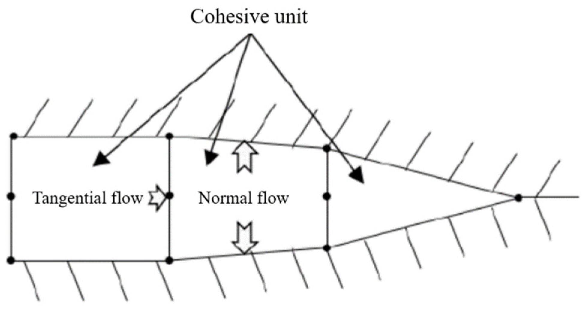
2.1.1. Cohesion Unit Model

The cohesive model uses fracture criteria to determine the damage condition. Damage occurs on cohesive units, and when the damage criterion is met, the unit starts to deteriorate. According to the predefined damage evolution model, when the unit completely fails, the mid layer of the unit “splits into two”, resulting in a geometric discontinuity and the formation of fractures.

A complete damage process can be divided into the initiation stage and the damage stage. In the initiation stage, as the tensile displacement increases, the traction force also increases. When it reaches the damage initiation point, the material begins to deteriorate, and the traction force starts to decrease until it reaches zero, and the fracture fully opens. Before damage occurs, the stress and strain satisfy the following relationship:

$$\sigma =\left\{\begin{array}{l}{\sigma }_n\\ {\sigma }_s\\ {\sigma }_t\end{array}\right\}=\left[\begin{array}{lll}{K}_{nn}& K_{ns}& K_{nt}\\ K_{sn}& K_{\mathrm{ss}}& K_{st}\\ K_{tn}& K_{\mathrm{ts}}& K_{tt}\end{array}\right]\left\{\begin{array}{l}{\epsilon }_n\\ {\epsilon }_s\\ {\epsilon }_t\end{array}\right\}=K\epsilon$$

(1)

where $\sigma$ is the stress vector, $Pa$; ${\sigma }_n$ is the normal stress of the element, $Pa$; ${\sigma }_s$ is the first shear stress, $Pa$; ${\sigma }_t$ is the second shear stress (which does not exist in the two-dimensional case), $Pa$; $K$ is the stiffness matrix of the element, dimensionless; $\epsilon$ is the strain, dimensionless; ${\epsilon }_n$ is the strain generated in the normal direction of the element, dimensionless; ${\epsilon }_s$ is the strain generated in the first shear direction, dimensionless; and ${\epsilon }_t$ is the strain generated in the second shear direction, dimensionless. The expression is as follows:

$${\epsilon }_n=\frac{d_n}{T_0},{\epsilon }_s=\frac{d_s}{T_0},{\epsilon }_t=\frac{d_t}{T_0}$$

(2)

where $d$ is displacement, $m$, and $T_0$ is the constitutive thickness, dimensionless.

The damage model is used to describe the stiffness degradation and structural failure of a material after the traction force reaches its maximum critical value. The damage model consists of two parts: damage initiation criteria and damage evolution laws. Once the damage reaches the damage initiation criteria, the failure will occur according to the defined damage evolution laws. In this case, the damage initiation criteria used is the maximum nominal stress criterion.

$$f=\max \left\{\frac{\left[t_n\right]}{t_n^0},\frac{t_s}{t_s^0},\frac{t_t}{t_t^0}\right\}$$

(3)

where $t_n^0$ is the traction force perpendicular to the fracture surface at the beginning of damage, $N$; $t_s^0$, $t_t^0$ is the traction force perpendicular to the fracture surface at the beginning of damage, $N$; $t_n$ is the traction force perpendicular to the fracture surface, $N$; $t_s$, $t_t$ is the traction force perpendicular to each other on the fracture surface, $N$; and $f$ is the fracture criterion, and fracture will occur when $1.0\le f\le 1.0+f_{tol}$; $f_{tol}$ is the tolerance, with a default value of 0.05.

The evolution law of damage describes the rate of the stiffness degradation of a material once it reaches the corresponding initiation criteria. The overall damage of the material is represented by $D$, with an initial value of 0, indicating no damage. After the initiation of damage, $D$ monotonically changes to 1, indicating complete failure. The stress components are represented as follows:

$$t_n=\left\{\begin{array}{l}\left(1-D\right)\overline{t_n} \overline{t_n}\ge 0\\ \overline{t_n} \hspace{1em}\overline{t_n}<0\end{array}\right\}$$

(4)

$$t_s=\left(1-D\right)\overline{t_s}$$

(5)

$$t_t=\left(1-D\right)\overline{t_t}$$

(6)

Among them, $\overline{t_n}$, $\overline{t_s}$, and $\overline{t_t}$ are the stresses in the normal and two tangential directions predicted based on the current strain using the linear damage evolution criterion, $Pa$, respectively.

The expression for the damage factor in the linear damage evolution criterion is as follows:

$$D=\frac{d_m^f\left(d_m^{\max }-d_m^0\right)}{d_m^{\max }\left(d_m^f-d_m^0\right)}$$

(7)

where $d_m^f$ is the displacement at the complete failure of the element, $m$; $d_m^{\max }$ is the maximum displacement of the element, $m$; and $d_m^0$ is the displacement of the unit at the beginning of damage, $m$.

In general, the fracture propagation form is a mixed mode of normal and tangential expansion.

When defining the mixed mode for cohesive elements using a power-law form, the relationship between $G_n$, $G_s$, and $G_t$ should satisfy:

$${\left\{\frac{G_n}{G_n^C}\right\}}^{\alpha }+{\left\{\frac{G_s}{G_s^C}\right\}}^{\alpha }+{\left\{\frac{G_t}{G_t^C}\right\}}^{\alpha }=1$$

(8)

where $G_n^C$ is the normal fracture energy of the cohesive element, $MPa\cdot m^{1/2}$; $G_s^C$ is the first shear fracture energy of the cohesive element, $MPa\cdot m^{1/2}$; $G_t^C$ is the second shear fracture energy of the cohesive element, $MPa\cdot m^{1/2}$; and $\alpha$ is the exponential coefficient, dimensionless. If the equation holds true, then the total fracture energy of cohesive elements in the mixed mode is equal to $G^C=G_n+G_s+G_t$.

When defining the mixed mode for cohesive elements using the BK form, if we assume that the first mode fracture energy and the second mode fracture energy of the cohesive element are equal, then the relationship between $G_n$, $G_s$, and $G_t$ should satisfy the following:

$$G_n^C+\left(G_s^C-G_n^C\right)\left\{\frac{G_s+G_t}{G_n+G_s+G_t}\right\}=G^C$$

(9)

2.1.2. The Fluid Flow Properties within a Fracture Surface

During the hydraulic fracturing process, the length and height of the fracture are much larger than the width, so the fluid flow within the fracture can be considered as a continuous flow between two porous plates. Assuming the fluid within the fracture is incompressible, the flow within the cohesive unit mainly exhibits two modes: a. tangential flow along the direction of the cohesive unit and b. normal flow perpendicular to the surface of the cohesive unit, along the upward and downward directions, as shown in Figure 1.

Assuming the injected fracturing fluid during the hydraulic fracturing process is a Newtonian fluid and the injection rate $q$ remains constant, the tangential flow of the fluid along the fracture propagation direction can be defined by Newtonian fluid pressure conduction:

$$Q=-k_t\Delta p$$

(10)

where $Q$ is the displacement of fracturing fluid, ${\mathrm{m}}^3/\mathrm{s}$; $k_t$ is the flow coefficient, dimensionless; and $p$ is the flow pressure, $\mathrm{MPa}$.

According to the Reynolds number equation, the flow coefficient $k_t$ can be represented as follows:

$$k_t=\frac{d^2}{12\mu }$$

(11)

where $d$ is the fracture opening displacement, $m$ and $\mu$ is the viscosity coefficient of the fracturing fluid, $\mathrm{Pa}·\mathrm{s}$.

The surface filtration characteristics of porous media can be defined as the flow of fracturing fluid in the normal direction. The seepage filtration loss of the fracturing fluid injected during the hydraulic fracturing process can be characterized by setting the filtration coefficient of cohesive elements. During the fracturing process, only a small portion of the fluid in the fracture will penetrate into the formation through the surface of the cohesive elements. The seepage flow in the direction perpendicular to the fracture surface can be expressed as follows:

$$\left\{\begin{array}{l}{q}_t=c_t(p_i-p_t)\\ q_b=c_b(p_i-p_b)\end{array}\right\}$$

(12)

where $q_t$, $q_b$ is the seepage flow rate of the fluid on the upper and lower surfaces of the fracture, ${\mathrm{m}}^3/\mathrm{s}$; $c_t$, $c_b$ is the filtration coefficient of the fluid on the upper and lower surfaces of the fracture, $\mathrm{m}/\mathrm{Pa}·\mathrm{s}$; $p_t$, $p_b$ is the pore pressure of the fluid on the upper and lower surfaces of the fracture, $\mathrm{MPa}$; and $p_i$ is the fluid pressure on the mid surface of the cohesive fracture element, $\mathrm{MPa}$.

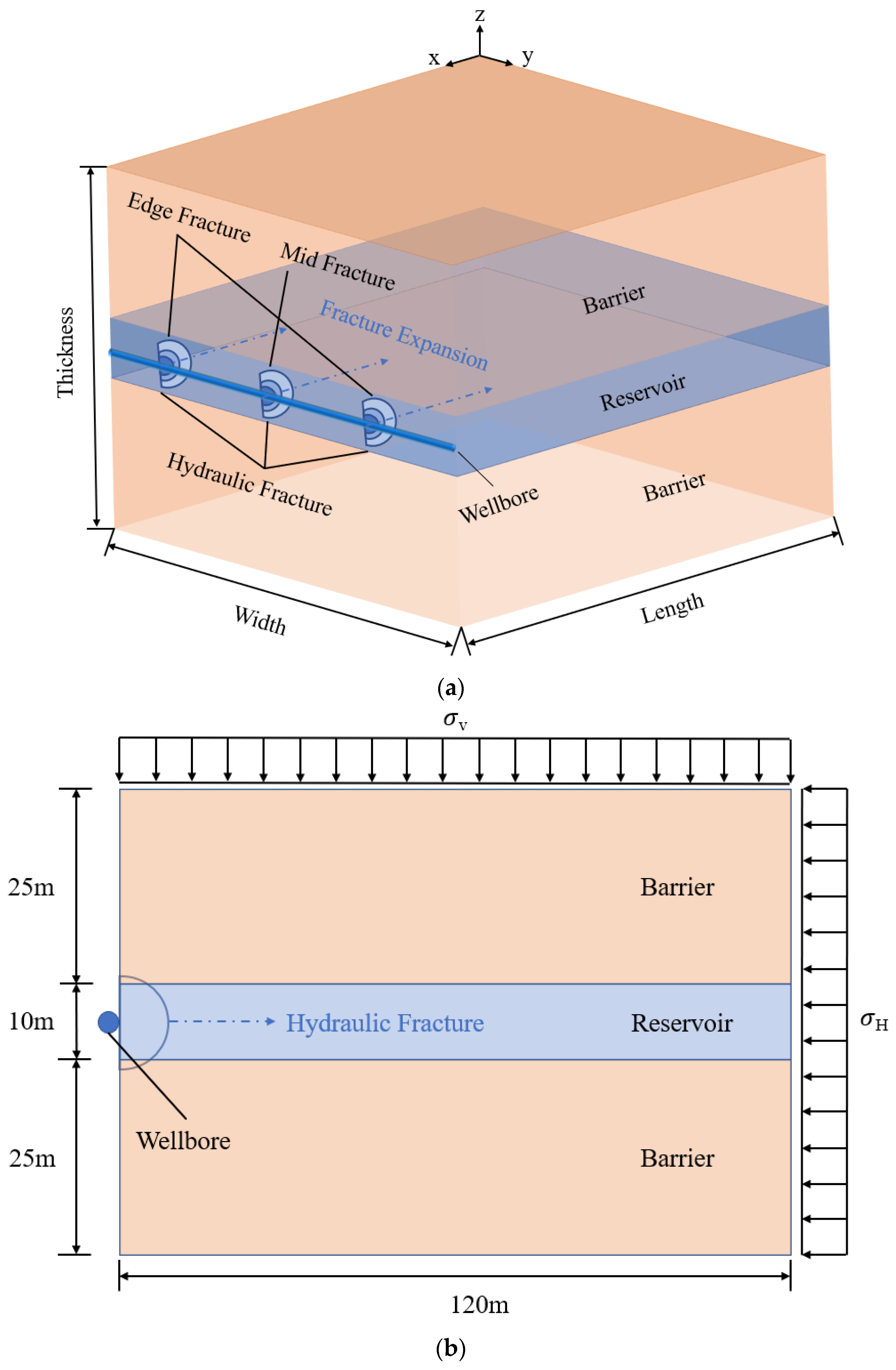
2.2. Model Configuration

The target formation is located in the western region of China. The lithology of this reservoir is highly variable, composed of various mineral components. The upper part of the formation consists mainly of litharenite, lithic feldspar fine sandstone, litharenite sandstone, and argillaceous fine sandstone. The target interval is distributed between 3100 m and 3350 m. Based on well logging data and rock mechanics experiments, the factors influencing fracture propagation during the multi-cluster fracturing process were studied, and a model was established as shown in Figure 2.

During the actual hydraulic fracturing process, rocks are subjected to highly complex geological conditions. In order to facilitate calculation and analysis in establishing the hydraulic fracturing model, the following assumptions need to be made:

• The formation rock is assumed to be a homogeneous and isotropic porous medium, and it is in a linear elastic state.
• The influence of temperature field on fracture propagation is neglected.
• The inertial effects of the fluid are disregarded.
• The fracturing fluid is fully saturated and incompressible. During the fracturing process, the physical and chemical interactions between the fracturing fluid and the surrounding rock formation are not considered.

A three-dimensional model was created using the finite element method (FEM). The initial dimensions of the model were set to 120 m 60 m 120 m. Three injection points, or perforations, were initially set up with a spacing of 20 m between each point. The formation consists of three layers, with the mid layer being the reservoir with a thickness of 10 m, and the upper and lower layers acting as interlayers with a thickness of 25 m each. The x direction represents the direction of maximum principal stress, the y direction represents the direction of minimum principal stress, and the z direction represents the direction of vertical stress. The fractures propagate in the direction of maximum principal stress. Therefore, cohesive elements were embedded in the xoz plane to simulate the initiation and propagation of fractures in the reservoir. The model was refined with a finer mesh in the mid reservoir layer, and to account for the influence of the interlayer, a 5 m region near the reservoir on both sides of the interlayer was also refined, while the rest of the mesh was relatively sparse, totaling 93,000 grid cells. The rock elements of the formation were set as C3D8P, and the cohesive elements representing the pre-existing fractures were set as COH3D8P. Displacement constraints of 0 were applied in all directions. The total duration of the hydraulic fracturing process was set to 400 s. The simulation of the hydraulic fracturing process mainly consists of two steps: (1) the equilibrium stage of the in situ stresses, and (2) the hydraulic fracturing stage. The basic calculation parameters are shown in

Table 1. Basic parameters for model calculation.

Reservoir	Elastic modulus/GPa	12
	Poisson’s ratio	0.18
	Permeability coefficient/m·s−1	1 × 10−7
	Porosity ratio	0.11
	Filtration coefficient/m·(Pa·s)−1	1 × 10−13
Interlayer	Elastic modulus/GPa	18
	Poisson’s ratio	0.13
	Permeability coefficient/m·s−1	1 × 10−8
	Porosity ratio	0.03
	Filtration coefficient/m·(Pa·s)−1	1 × 10−14
Other parameters	Tensile strength/MPa	6
	Pore pressure/MPa	28
	Displacement/m2·s−1	0.01
	Viscosity/Pa·s	0.001

.

The PKN (Perkins–Kern–Nordgren) model [14,15,34] is one of the classic models used to describe crack propagation during hydraulic fracturing. It assumes that the expansion of cracks can be approximated by an ellipsoid or ellipsoidal volume. The core idea behind this model is the pattern of crack expansion under the influence of hydraulic fracturing, particularly applicable when the cracks have a relatively large length-to-width ratio. Before initiating multi-fracture propagation simulations, we conducted simulations of a single crack and compared the results with those calculated using the PKN model, as shown in Figure 3.

To ensure the convergence of the model, a ramp-up injection amplitude was applied to the volume before the start of fracturing, gradually increasing the fracturing volume from 0 to the set value within the first 20 s. Therefore, the results obtained from the simulation before 20 s show relatively small differences but are generally consistent. After 20 s, the width and length of the fracture begins to increase. The fracture width obtained from the simulation is consistent with the results from the PKN model calculations, while the length shows minor differences. Hence, the simulation results provide a certain level of reference and reliability.

3. Results

The expansion of fractures exhibits symmetry, with both sides of the fracture (referred to as “edge fracture” hereafter) behaving similarly. Therefore, the analysis focuses on the expansion behavior of one edge fracture and the central fracture (referred to as “mid fracture” hereafter). Figure 4 illustrates the expansion of the mid fracture and edge fracture at 30 s, 200 s, and 400 s. It can be observed that in the initial stage of fracture propagation, there is little difference in the morphology of the two fractures. As time progresses, the mid fracture becomes longer and narrower, while the edge fracture becomes wider and shorter. Additionally, the mid fracture exhibits less fracture compared to the edge fracture. This is because during expansion, the edge fractures on both sides exert a compressive effect on the mid fracture, limiting its expansion towards the sides while promoting its forward expansion.

Figure 5 reflects the variation in pore pressure at the injection points during fracture expansion. The edge fracture injection point ruptures and fracture expansion begins when the pore pressure reaches 47.85 MPa, while the mid fracture pore pressure needs to reach 49.31 MPa for fracture expansion to start. Therefore, the edge fracture expands before the mid fracture, exerting a certain suppression effect on the width of the mid fracture and promoting its length. Additionally, the forward expansion of the mid fracture also has a certain inhibitory effect on the expansion of the edge fractures on both sides. As the fractures continue to expand, the pore pressure at the mid fracture injection point and the edge fracture injection point eventually stabilize at around 23.37 MPa and 24.34 MPa, respectively.

4. Discussion

In this section, six parameters were selected to analyze their influence on the morphology of fracture propagation. These parameters include three hydraulic fracturing construction parameters (cluster spacing, cluster count, and displacement) and three geomechanical parameters (elastic modulus, Poisson’s ratio, and permeability). To reflect the role of the interlayer in hydraulic fracturing simulation, the values of geomechanical parameters are taken as the ratio of interlayer parameters to reservoir parameters. The stimulated reservoir volume (SRV) in the reservoir and interlayer under the influence of each parameter was extracted, and the reasons for the differences were analyzed and discussed.

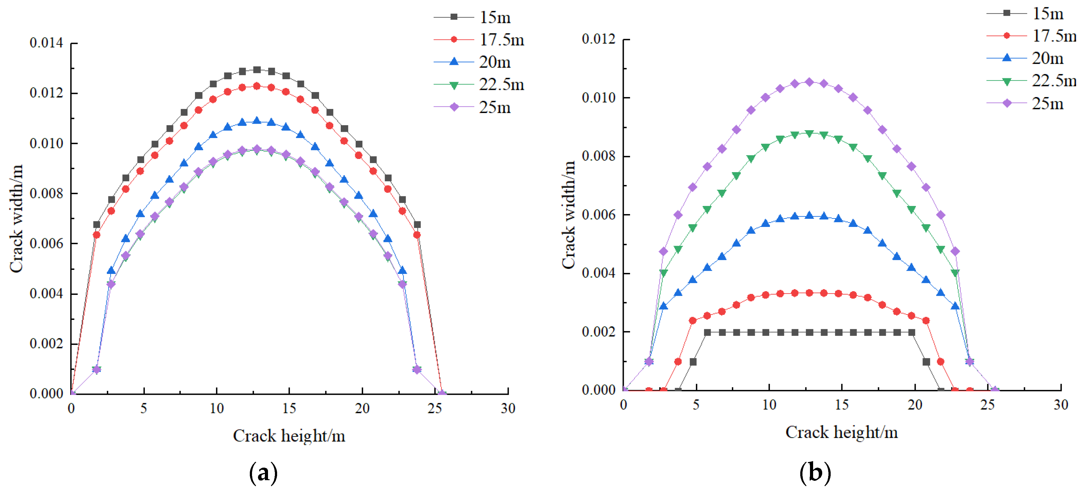
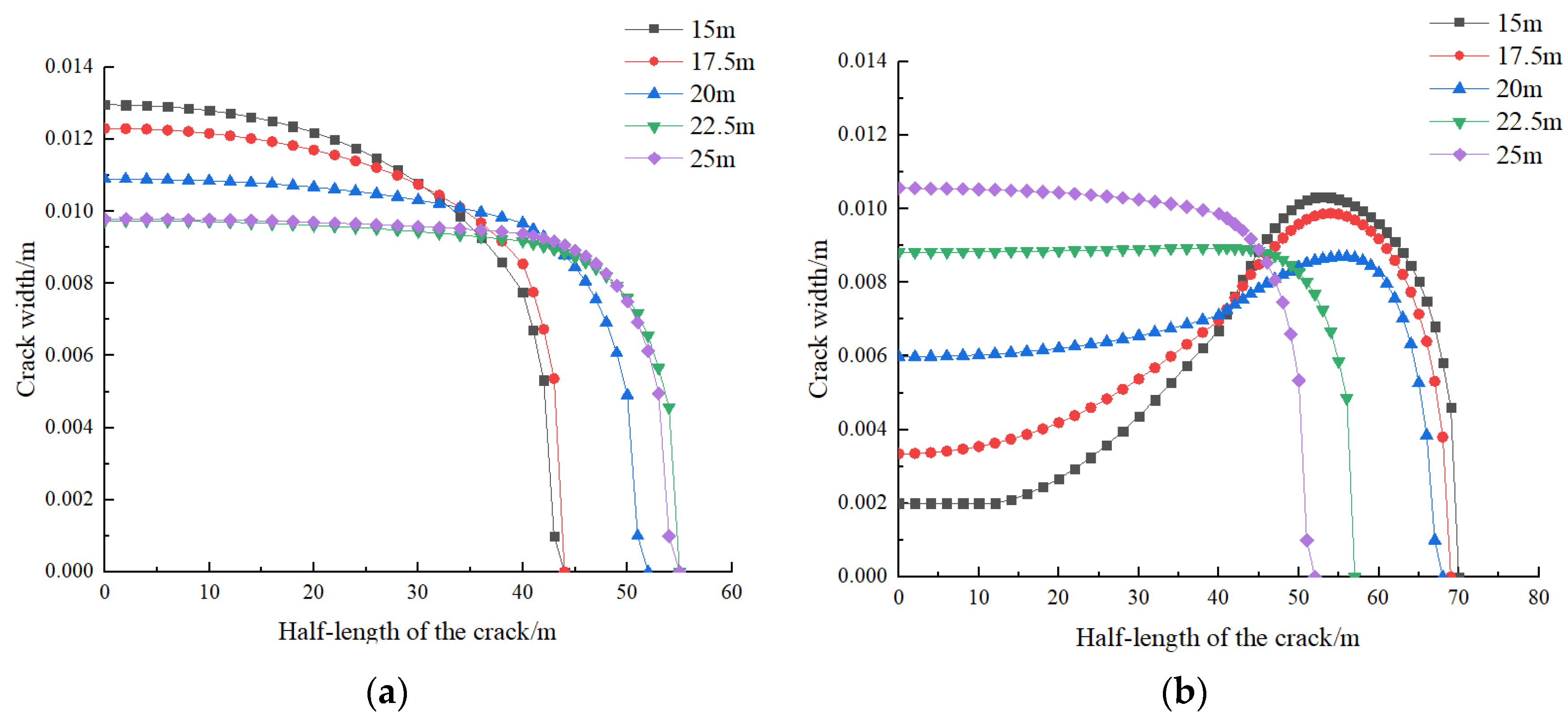
4.1. Effect of Cluster Spacing

Keeping other parameters constant, three pre-existing fractures are established with distances between fractures of 15 m, 17.5 m, 20 m, 22.5 m, and 25 m, respectively. The influence of different cluster spacing conditions on fracture morphology is analyzed and studied. The simulation results are shown in Figure 6 and Figure 7.

From Figure 6, it can be observed that the height of the edge fracture reaches its maximum value. The fracture width–height curves show little difference between cluster spacings of 15 m and 17.5 m. The curves for cluster spacings of 22.5 m and 25 m overlap each other. The height of the mid fracture increases with the increase in cluster spacing. The compression effect is minimal at a cluster spacing of 25 m, resulting in the maximum fracture width. The compression effect is maximum at a cluster spacing of 15 m, resulting in the smallest fracture width, and the height does not reach its maximum value. As the cluster spacing increases, the fracture width increases, reaching its maximum at a cluster spacing of 25 m. When the cluster spacing is too small, there is a significant difference in the width of the mid fracture, with a difference of 81% between the maximum and minimum widths. In contrast, the difference between the maximum and minimum widths of the edge fracture is only 24%.

Figure 7 illustrates the relationship between fracture width and half-length. When the cluster spacing is 15 m and 17.5 m, the initial width of the mid fracture is small and the half-length is long due to the compression effect from the edge fracture. As the fracture half-length increases, the influence of the edge fracture on the mid fracture weakens, resulting in an increasing width. At the front end of fracture propagation, the width decreases to zero. The edge fracture, on the other hand, has a shorter fracture half-length due to the influence of fluid loss into the formation during the expansion of the mid fracture, but it has a larger initial width. When the cluster spacing is 20 m, 22.5 m, and 25 m, the compression effect on the mid fracture weakens, leading to an increased initial width and more fluid loss into the formation. As a result, the fracture half-length decreases. The difference in the fracture width–half-length curves is not significant between cluster spacings of 22.5 m and 25 m. The influence of fluid loss into the formation at the front end of the fracture from the mid fracture weakens the compression effect on the edge fracture, resulting in the curves of fracture width–half-length for the edge fracture and the mid fracture overlapping each other.

When the fracture spacing is small, the edge fracture has a significant impact on the mid fracture. As the fracturing fluid is continuously injected, the edge fracture exerts compression on the mid fracture. This causes the width of the injection point of the mid fracture to decrease, while the width of the injection point of the edge fracture is larger. However, under the action of the fracturing fluid, the force for the mid fracture to expand forward increases, resulting in a longer half-length compared to the edge fracture. At the same time, the fracturing fluid loss into the formation at the front end of the mid fracture hinders the forward expansion of the edge fracture to some extent, resulting in a shorter half-length for the edge fracture. As the cluster spacing increases, the mutual compression between the fractures weakens, and the mutual influence of pore pressure decreases. The widths of the injection points and the half-lengths of the three fractures tend to be consistent.

4.2. Effect of Cluster Quantity

Keeping other parameters constant, when the inter-cluster spacing is 20 m, the number of perforations is set to 1, 2, 3, 4, and 5, respectively. Different numbers of pre-existing fractures are created, with the fractures propagating in the same direction as the maximum principal stress. The morphology and extension of the fractures under different cluster quantities are analyzed and studied. The simulation results are shown in Figure 8 and Figure 9.

Figure 8 reflects the relationship between the width and height of edge/mid fractures. Since there is no clear division between edge and mid fractures when there is one cluster or two clusters, a comparison is made between the fracture morphology in these two cases and the other cases. It can be observed that for edge fractures, the height of the fracture reaches the maximum in all five cases. The width is maximum when there is one cluster, indicating a normal extension behavior of the fracture without the influence of other fractures. When there are two clusters, the width is minimum, as the two fractures expand simultaneously and interact with each other. The remaining three cases have curves located between the curves of one cluster and two clusters. The expansion of the front end of the mid fracture hinders the extension of the front end of the edge fracture due to the loss of fracturing fluid into the formation. The fracturing fluid in the edge fracture mainly affects the width expansion, resulting in a larger maximum width compared to one cluster and two clusters. The other three curves overlap, indicating consistent influence on the edge fracture, with a maximum difference of 13% between the curves. For mid fracture, the maximum width decreases in the order of one cluster, two clusters, four clusters, three clusters, and five clusters. The width of three clusters is smaller than four clusters because the mid fracture in three clusters is influenced by the two adjacent edge fractures, while the mid fracture in four clusters is influenced by one edge fracture on one side and another mid fracture on the other side, with the influence of the other mid fracture being smaller than that of the edge fracture. Therefore, the mid fracture in three clusters is more affected by the two edge fractures and has a smaller width compared to four clusters. The height of the fractures in four clusters and five clusters does not reach the maximum, with a maximum difference of 56% between the curves.

Figure 9 reflects the relationship between the width and half-length of edge/mid fractures. The expansion pattern of width–half-length for edge fractures is consistent with the expansion pattern of width–height, and the width of the fracture increases while the half-length decreases. When there is one cluster or two clusters, the width of the mid fracture decreases with the increase in the half-length. When there are three clusters, four clusters, and five clusters, the width of the fracture initially increases and then decreases with the increase in the half-length. This indicates that the mid fracture in three clusters, four clusters, and five clusters is initially more influenced by the edge fracture, resulting in a smaller width. The fracturing fluid mainly promotes the forward expansion of the fracture, and as the half-length of the fracture increases, the width increases. When the mid fracture is no longer influenced by the edge fracture, the width of the fracture increases.

When the cluster spacing is 20 m with three clusters, interactions between the edge and central clusters begin to affect each other. To better reflect the varying degrees of interaction between the edge and central clusters when other parameters change, the upcoming model will use a cluster spacing of 20 m with three clusters.

4.3. Effect of Displacement

Keeping other parameters constant, the displacement ratio of fracturing fluid was changed sequentially to 1, 1.1, 1.2, 1.3, and 1.4 to study the effect of fracturing fluid displacement on the morphology of fracture propagation. The simulation results are shown in Figure 10 and Figure 11.

From Figure 10 and Figure 11, it can be observed that, under the same injection time, as the displacement of fracturing fluid increases, the width, height, and half-length of the edge fracture increase at the end of the fracturing process, while the width of the mid fracture decreases and the height and half-length increase. Normally, most of the injected fracturing fluid is used for the extension and propagation of fractures, with only a small portion lost into the formation. As the fracturing fluid is injected, the fractures will expand in three dimensions. However, due to the increase in fracturing fluid displacement, the portion lost into the formation also increases, affecting the mid fracture by inhibiting the increase in its width. Since the injected volume of fracturing fluid is the same, the fracturing fluid in the mid fracture mainly contributes to the forward extension of the fracture. Therefore, with a larger displacement, the width of the mid fracture becomes smaller while the half-length becomes longer. Generally, the fracture width opens along the direction of minimum principal stress, and compared to the half-length and height of the fracture, a greater resistance needs to be overcome. Hence, the fracture width is smaller than the half-length and height of the fracture.

With the increase in displacement, the volume of fracturing fluid injected into the formation within the same time period is larger, resulting in more fluid loss into the formation. This leads to a greater interaction between the fractures. The larger displacement will increase the length and width of the fractures, while the squeezing effect of the edge fracture on the mid fracture becomes more pronounced. As a result, the width of the mid fracture decreases, the half-length increases, and the difference in half-length between the mid fracture and edge fracture also increases. However, the degree of fracturing in the mid fracture is not as significant as in the edge fracture.

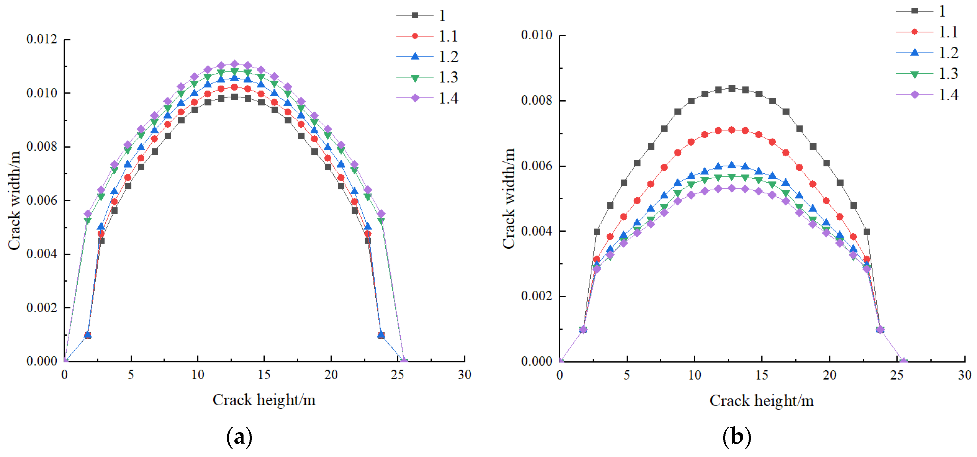
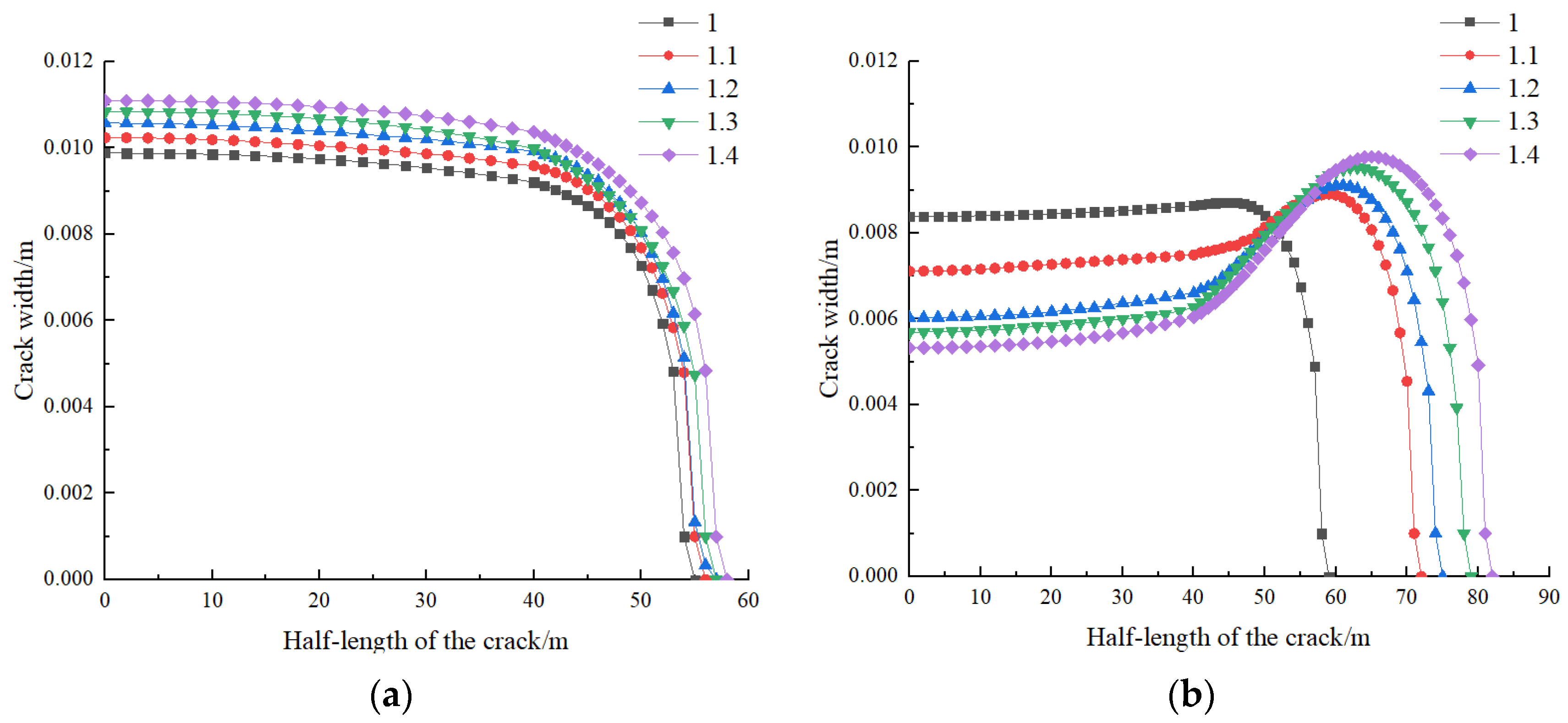
4.4. Effect of Elastic Modulus

Keeping other parameters constant, the ratio of elastic modulus between the interlayer and reservoir is set to 1.5, 2, 2.5, 3, and 3.5. The simulation results are shown in Figure 12 and Figure 13.

Figure 12 illustrates the relationship between the width and height of the edge and mid fractures under different elastic modulus ratios. It can be observed that as the elastic modulus ratio increases, the maximum width of the edge fracture decreases, and the differences between adjacent curves decrease. If the elastic modulus ratio continues to increase, the maximum width of the edge fracture may tend towards a constant value. The elastic modulus ratio at which the maximum width of the mid fracture stabilizes is reached relatively quickly. When the elastic modulus ratio is 1.5, the maximum width of the mid fracture is at its minimum value, and there is little difference in the maximum width among the other four cases.

Figure 13 depicts the relationship between the width of the edge and mid fractures and their half-lengths under different elastic modulus ratios. It can be observed that under different elastic modulus ratios, the width of the edge fracture is negatively correlated with the half-length. The smaller the width, the larger the half-length, and the rate of decrease in fracture width decreases. Meanwhile, the increment of fracture half-length remains almost stable. For the mid fracture, when the elastic modulus ratio is 1.5, the fracture width initially increases and then decreases with the increase in half-length. There is little difference in the width–half-length curve among the other four cases, and as the fracture width increases, the fracture half-length decreases.

As the elastic modulus ratio increases, the influence on the fractures becomes more significant. Increasing the ratio of elastic modulus will inhibit the extension of cracks in the vertical direction. The expansion of cracks in the vertical direction is impeded. Under the condition that the amount of fracturing fluid injection remains constant, this will cause the cracks to expand forward and increase the half-length of the cracks. The increase in half-length of the edge fracture and the decrease in the degree of fracture propagation are quite noticeable. The half-length of the mid fracture decreases but gradually approaches a stable value, while the degree of fracture propagation increases. However, the overall degree of fracture propagation decreases with the increase in the elastic modulus ratio, and the pore pressure in the model increases with the increase in the elastic modulus ratio. When the elastic modulus ratio is two, the half-length of the edge and mid fracture are comparable, and the degree of fracture propagation is relatively good.

4.5. Effect of Poisson’s Ratio

Keeping other parameters constant, the ratio of Poisson’s ratio between the interlayer and reservoir is set to 0.7, 1, 1.3, 1.6, and 1.9. The simulated results are shown in Figure 14 and Figure 15.

From Figure 14, it can be observed that when the ratio of Poisson’s ratio between the interlayer and reservoir is 0.7, the maximum width of the edge fracture is 0.0109 m, while the maximum width of the mid fracture is only 0.006 m. As the ratio increases, the maximum width of the edge fracture decreases. After the ratio reaches one, the maximum width remains relatively consistent, with a minimum value of 0.0094 m and a small decrease. The maximum width of the mid fracture increases, and after the ratio reaches one, it also remains relatively consistent, with a maximum value of 0.0093 m. The increase is initially significant and then stabilizes. As the ratio becomes larger, the maximum widths of the edge fracture and mid fracture are essentially the same.

From Figure 15, it can be observed that as the ratio increases, the width of the edge fracture decreases while the half-length increases. On the other hand, the width of the mid fracture increases while the half-length decreases. The decrease in the width of the edge fracture is relatively small and tends to stabilize, while the increase in the width of the mid fracture is initially significant and then stabilizes. When the ratio reaches 1.9, both the edge fracture and mid fracture have a half-length of 56 m, and the trend of the curves is basically consistent.

As the ratio of the Poisson’s ratio between the interlayer and reservoir increases, the horizontal deformation of the rock is larger while the vertical deformation is relatively smaller. In the case of the constant injection of fracturing fluid, the cracks are more difficult to expand in the vertical direction and instead tend to expand in the semi-longitudinal direction of the crack, the overall degree of fracture of the fractures decreases, but the decrease is relatively small. The half-length of the mid fracture decreases, but its degree of fracture increases. With the increase in the ratio, the half-length of the mid fracture becomes almost equal to the half-length of the edge fracture.

4.6. Effect of Permeability

Keeping other parameters constant, the ratio of permeability between the interlayer and the reservoir is set to 0.5, 1, 1.5, 2, and 2.5. The simulation results are shown in Figure 16 and Figure 17.

Figure 16 and Figure 17, respectively, illustrate the relationship between fracture width and height, as well as the relationship between width and half-length, under different permeability ratios. As the permeability ratio increases, the maximum fracture width of the edge and mid fracture also increases. The influence on the edge fracture is relatively small, with a maximum width ranging from 0.011 m to 0.0104 m, showing little difference. When the permeability ratio is relatively small, the influence on the mid fracture is significant. However, as the permeability ratio increases, the influence on the mid fracture weakens. The maximum width of the mid fracture ranges from 0.0113 m to 0.0063 m. When the permeability ratio is large, there is not much difference in the maximum fracture width between the edge fracture and mid fracture. The fracture width is negatively correlated with the half-length. As the permeability ratio increases, the fracture width increases while the half-length decreases. The influence on the edge fracture is relatively small, while the influence on the mid fracture is significant when the permeability ratio is relatively small. In this case, the fracture width initially increases and then decreases with the half-length. As the permeability ratio continues to increase, the influence on the mid fracture becomes smaller. When the permeability ratio is large, the half-length of the edge fracture and mid fracture is approximately 51 m and 49 m, respectively, showing little difference.

As the permeability ratio increases, the influence on the fracture morphology of the mid fracture is significant, resulting in a decrease in the half-length. The influence on the fracture morphology of the edge fracture is not significant. The increase in permeability ratio leads to less fracturing fluid entering the reservoir, resulting in a decrease in reservoir pore pressure and an increase in the degree of fracture rupture increases.

4.7. Effect of Various Factors on the SRV of the Interlayer/Reservoir

When the fractures are close to each other, there is strong interference between them, causing mutual compression and leading to the fractures tending to expand vertically. As a result, the stimulated reservoir volume (SRV) in the interlayer is larger than that in the reservoir. When the cluster spacing is 20 m, the mutual compression between fractures suddenly decreases, resulting in an increase in the SRV in the reservoir and a decrease in the SRV in the interlayer. With increasing spacing, the total SRV gradually stabilizes (Figure 18a).With an increase in the number of clusters, the SRV in both the reservoir and interlayer increases simultaneously (Figure 18b). A larger displacement leads to a larger SRV. As the displacement increases, the volume of fracturing fluid lost into the formation increases, which has a greater impact on the mid fracture. The degree of fracture rupture in the mid fracture in the interlayer is less than that in the edge fracture. However, the volume of fractures expanding in the interlayer for the edge fracture is larger than that for the mid fracture. Therefore, with an increase in displacement, the SRV in the interlayer exceeds that in the reservoir (Figure 18c). A larger elastic modulus indicates a stronger resistance to deformation in the rock, resulting in a decrease in the total SRV. However, as the ratio of elastic modulus between the interlayer and reservoir increases, the SRV in the reservoir slightly increases, while the decrease in the SRV in the interlayer is more significant, which is beneficial for reservoir exploitation (Figure 18d). As the ratio of Poisson’s ratio and permeability between the interlayer and reservoir increases, the SRV in the reservoir slightly decreases, while the SRV in the interlayer slightly increases, with minimal impact on actual exploitation, which can be essentially ignored (Figure 18e,f).

5. Conclusions

This study uses a cohesive element model to investigate the morphological characteristics of hydraulic fracturing with multiple clusters. It discusses the research and analyzes the effects of three fracturing construction parameters (cluster spacing, the number of clusters, and displacement) and three geomechanical parameters (elastic modulus, Poisson’s ratio, and permeability) on the behavior, morphology, and stimulated reservoir volume (SRV) of fracture propagation. The main conclusions are as follows:

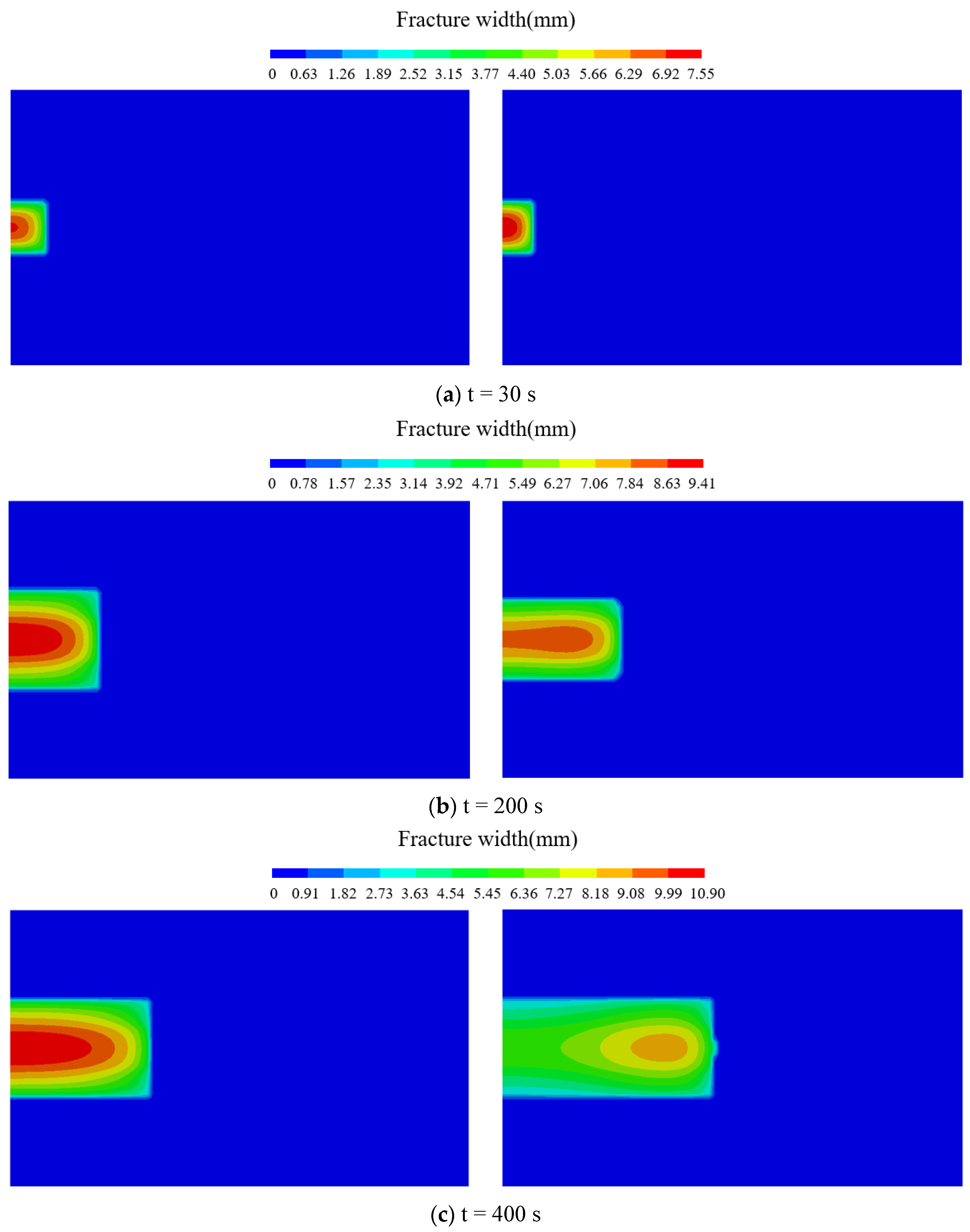
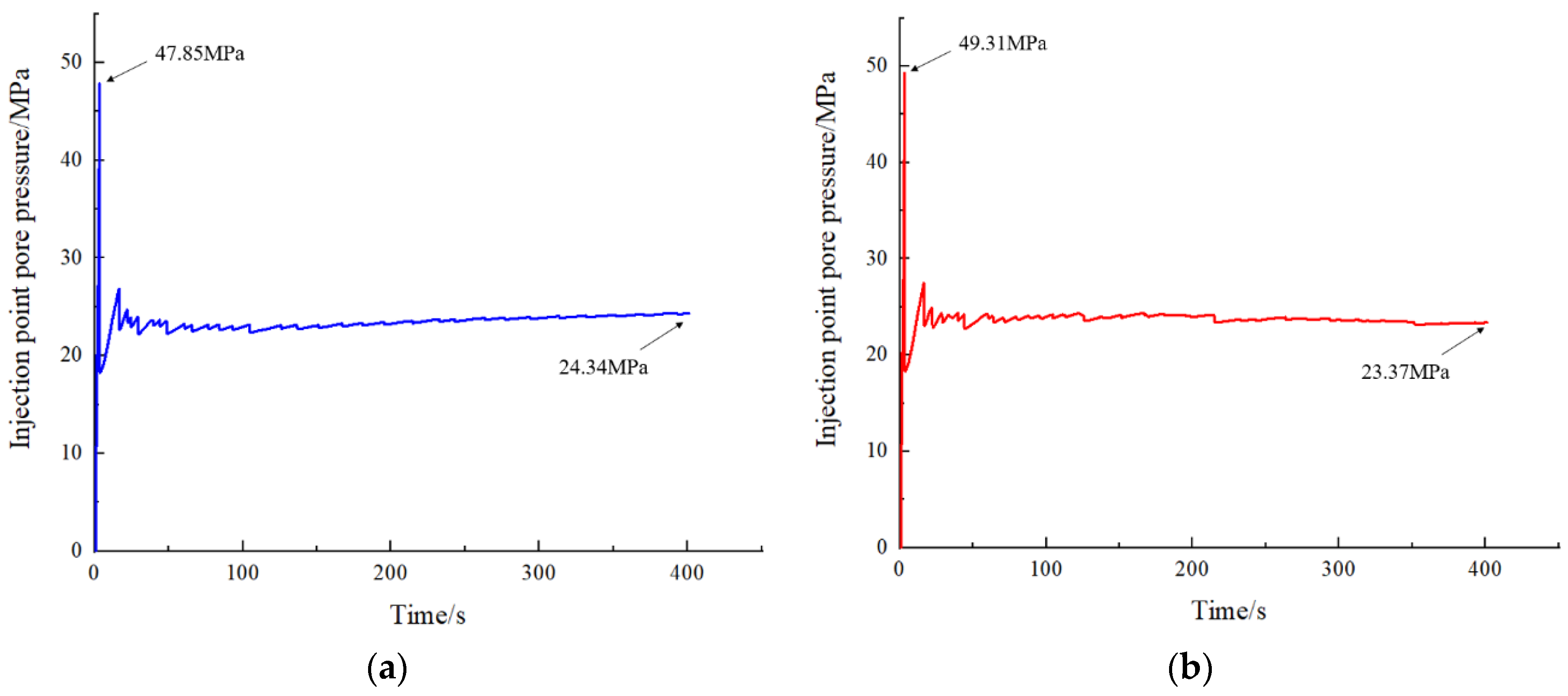
• At the initial stage of fracturing, the edge fracture starts to propagate when the injection pressure reaches 47.85 MPa, while the mid fracture starts to propagate at an injection pressure of 49.31 MPa. This indicates that there is a certain interaction between the fractures during the fracturing process. The propagation of the mid fracture in terms of width and height is influenced by the edge fracture. With the same amount of fracturing fluid injection, the length of the mid fracture will be greater than that of the edge fracture.
• When the cluster spacing is small, the mid fracture is greatly influenced by the edge fracture, resulting in a lower height and narrower width than the predetermined maximum values. As the cluster spacing increases, the width and height of the mid fracture increase, while the length decreases. The situation is the opposite for the edge fracture. The more clusters there are, the more pronounced the interaction between the fractures, especially the influence of the edge fracture on the mid fracture. With a larger displacement, more fracturing fluid enters the formation, resulting in an increased length, width, and height of the edge fracture. However, the mid fracture is influenced by the edge fracture, leading to a decrease in width and an increase in length.
• The elastic modulus has a significant impact on the edge fracture. As the ratio of elastic moduli increases, the width of the edge fracture decreases while the length increases. When the ratio of elastic moduli is small, the mid fracture is longer and narrower. When the ratio of elastic moduli is large, the length of the mid fracture decreases while the width increases, but the impact is relatively small. As the ratio of Poisson’s ratios increases, the morphology of the edge fracture changes less, while the width of the mid fracture increases and the length decreases. When the ratio of Poisson’s ratios reaches a certain value, the influence on the fractures is basically negligible. An increase in the ratio of permeabilities allows more fracturing fluid to enter the formation, reducing the interaction between fractures. This has a minimal impact on the edge fracture, while promoting a better expansion of the mid fracture.
• An increase in cluster quantity and displacement leads to an increase in the SRV in both the reservoir and the interlayer. As the cluster spacing increases, the interaction between fractures decreases, causing the fractures to transition from vertical expansion to forward expansion, resulting in a larger SRV in the reservoir. A higher ratio of elastic moduli leads to a decrease in the overall SRV, but an increase in the SRV in the reservoir and a decrease in the SRV in the interlayer. This is beneficial for reservoir exploitation. The ratio of Poisson’s ratios and the ratio of permeabilities between the interlayer and the reservoir have a relatively small impact on the SRV in both the interlayer and the reservoir.

References

1. Mayerhofer, M.J.; Lolon, E.P.; Warpinski, N.R.; Cipolla, C.L.; Walser, D.; Rightmire, C.M. What Is Stimulated Reservoir Volume? SPE Prod. Oper. 2010, 25, 89–98. [Google Scholar] [CrossRef]
2. Chen, Q.; Wang, S.J.; Zhu, D.; Ren, G.X.; Zhang, Y.; Hu, J.H. A Comprehensive Model for Estimating Stimulated Reservoir Volume Based on Flowback Data in Shale Gas Reservoirs. Geofluids 2020, 2020, 8886988. [Google Scholar] [CrossRef]
3. Wang, H.Y. Numerical modeling of non-planar hydraulic fracture propagation in brittle and ductile rocks using XFEM with cohesive zone method. J. Pet. Sci. Eng. 2015, 135, 127–140. [Google Scholar] [CrossRef]
4. Guo, T.S.; Zhang, S.C.; Qu, Z.Q.; Zhou, T.; Xiao, Y.S.; Gao, J. Experimental study of hydraulic fracturing for shale by stimulated reservoir volume. Fuel 2014, 128, 373–380. [Google Scholar] [CrossRef]
5. Shi, D.Y.; Lu, Z.Y. Semianalytical Model for Flow Behavior Analysis of Unconventional Reservoirs with Complex Fracture Distribution. Geofluids 2020, 2020, 9394140. [Google Scholar] [CrossRef]
6. Yuan, B.; Su, Y.L.; Moghanloo, R.G.; Rui, Z.H.; Wang, W.D.; Shang, Y.Y. A new analytical multi-linear solution for gas flow toward fractured horizontal wells with different fracture intensity. J. Nat. Gas Sci. Eng. 2015, 23, 227–238. [Google Scholar] [CrossRef]
7. Zhang, M.Y.; Wang, D.Y.; Zhang, Z.L.; Zhang, L.Y.; Yang, F.; Huang, B.; Zhong, A.H.; Li, L.C. Numerical simulation and multi-factor optimization of hydraulic fracturing in deep naturally fractured sandstones based on response surface method. Eng. Fract. Mech. 2022, 259, 108110. [Google Scholar] [CrossRef]
8. Liu, X.Q.; Rasouli, V.; Guo, T.K.; Qu, Z.Q.; Sun, Y.; Damjanac, B. Numerical simulation of stress shadow in multiple cluster hydraulic fracturing in horizontal wells based on lattice modelling. Eng. Fract. Mech. 2020, 238, 107278. [Google Scholar] [CrossRef]
9. Hu, Y.Q.; Wang, Q.; Zhao, J.Z.; Chen, S.N.; Zhao, C.N.; Fu, C.H. Three-dimensional complex fracture propagation simulation: Implications for rapid decline of production capacity. Energy Sci. Eng. 2020, 8, 4196–4211. [Google Scholar] [CrossRef]
10. Zhang, K.P.; Chen, M.; Wang, S.G.; Li, J.X.; Taufiqurrahman, M. Significant effect of the rock parameters of Longmaxi formation in hydraulic fracturing. Geomech. Energy Environ. 2022, 32, 100384. [Google Scholar] [CrossRef]
11. Li, N.; Yang, K.; Kao, J.W. A new extended finite element model for gas flow in shale gas reservoirs with complex fracture networks. Arab. J. Geosci. 2023, 16, 503. [Google Scholar] [CrossRef]
12. Khristianovic, S.A.; Zheltov, Y.P. Formation of vertical fractures by means of highly viscous liquid. In Proceedings of the Fourth World Petroleum Congress, Rome, Italy, 6 June 1955. [Google Scholar]
13. Geertsma, J.; Klerk, F. A Rapid Method of Predicting Width and Extent of Hydraulically Induced Fractures. J. Pet. Technol. 1969, 21, 1571–1581. [Google Scholar] [CrossRef]
14. Perkins, T.K.; Kern, L.R. Widths of Hydraulic Fractures. J. Pet. Technol. 1961, 13, 937–949. [Google Scholar] [CrossRef]
15. Nordgren, R.P. Propagation of a Vertical Hydraulic Fracture. Soc. Pet. Eng. J. 1972, 12, 306–314. [Google Scholar] [CrossRef]
16. Settari, A.; Cleary, M.P. Development and Testing of a Pseudo-Three-Dimensional Model of Hydraulic Fracture Geometry. SPE Prod. Eng. 1986, 1, 449–466. [Google Scholar] [CrossRef]
17. Green, A.E.; Sneddon, I.N. The distribution of stress in the neighbourhood of a flat elliptical crack in an elastic solid. Math. Proc. Camb. Philos. Soc. 1950, 46, 159–163. [Google Scholar] [CrossRef]
18. King, G.E. Thirty Years of Gas Shale Fracturing: What Have We Learned? In Proceedings of the SPE Annual Technical Conference and Exhibition, Florence, Italy, 19–22 September 2010; Society of Petroleum Engineers: Florence, Italy, 2010. [Google Scholar] [CrossRef]
19. Cleary, M.P.; Michael, K.; Lam, K.Y. Development of a fully three-dimensional simulator for analysis and design of hydraulic fracturing. In Proceedings of the SPE /DOE Low Permeability Gas Reservoirs Symposium, Denver, Colorado, 14–16 March 1983. [Google Scholar] [CrossRef]
20. Shahid, A.S.A.; Fokker, P.A.; Rocca, V. A Review of Numerical Simulation Strategies for Hydraulic Fracturing, Natural Fracture Reactivation and Induced Microseismicity Prediction. Open Pet. Eng. J. 2016, 9 (Suppl. S1), 72–91. [Google Scholar] [CrossRef]
21. Lee, J.H.; Gao, Y.F.; Johanns, K.E.; Pharr, G.M. Cohesive interface simulations of indentation cracking as a fracture toughness measurement method for brittle materials. Acta Mater. 2012, 60, 5448–5467. [Google Scholar] [CrossRef]
22. Lecampion, B. An extended finite element method for hydraulic fracture problems. Commun. Numer. Methods Eng. 2009, 25, 121–133. [Google Scholar] [CrossRef]
23. Wang, W.R.; Zhang, G.Q.; Cao, H.; Chen, L.; Zhao, C.Y. Generation mechanism and influencing factors of fracture networks during alternate fracturing in horizontal wells. Theor. Appl. Fract. Mech. 2023, 127, 104082. [Google Scholar] [CrossRef]
24. Ma, J.Q.; Li, X.H.; Yao, Q.L.; Tan, K. Numerical simulation of hydraulic fracture extension patterns at the interface of coal-measure composite rock mass with Cohesive Zone Model. J. Clean. Prod. 2023, 426, 139001. [Google Scholar] [CrossRef]
25. Khoei, A.R.; Mortazavi, S.M.S.; Simoni, L.; Schrefler, B.A. Irregular and stepwise behaviour of hydraulic fracturing: Insights from linear cohesive crack modelling with maximum stress criterion. Comput. Geotech. 2023, 161, 105570. [Google Scholar] [CrossRef]
26. Wang, L.C.; Duan, K.; Zhang, Q.Y.; Li, X.J.; Jiang, R.H.; Zheng, Y. Stress interference and interaction between two fractures during their propagation: Insights from SCDA test and XFEM simulation. Int. J. Rock Mech. Min. Sci. 2023, 169, 105431. [Google Scholar] [CrossRef]
27. Xiong, J.; Liu, J.J.; Li, W.; Liu, X.J.; Liang, L.X.; Ding, Y. Investigation on the influence factors for the fracturing effect in fractured tight reservoirs using the numerical simulation. Sci. Prog. 2022, 105, 368504211070396. [Google Scholar] [CrossRef]
28. Chen, Z.R.; Jeffrey, R.G.; Zhang, X.; Kear, J. Finite-Element Simulation of a Hydraulic Fracture Interacting with a Natural Fracture. SPE J. 2017, 22, 219–234. [Google Scholar] [CrossRef]
29. Xia, B.W.; Ou, C.N.; Zhang, X.; Fu, Y.H. Expansion law and influence factors of hydraulic fracture under the influence of coal pillar. Arab. J. Geosci. 2021, 14, 961. [Google Scholar] [CrossRef]
30. Manchanda, R.; Sharma, M.M.; Holzhauser, S. Time-Dependent Fracture-Interference Effects in Pad Wells. SPE Prod. Oper. 2014, 29, 274–287. [Google Scholar] [CrossRef]
31. Wang, X.L.; Liu, C.; Wang, H.; Liu, H.; Wu, H.A. Comparison of consecutive and alternate hydraulic fracturing in horizontal wells using XFEM-based cohesive zone method. J. Pet. Sci. Eng. 2016, 143, 14–25. [Google Scholar] [CrossRef]
32. Wu, K.; Olson, J.E. Investigation of the Impact of Fracture Spacing and Fluid Properties for Interfering Simultaneously or Sequentially Generated Hydraulic Fractures. SPE Prod. Oper. 2013, 28, 427–436. [Google Scholar] [CrossRef]
33. Zhang, J.X.; Liu, X.J.; Wei, X.C.; Liang, L.X.; Xiong, J.; Li, W. Uncertainty Analysis of Factors Influencing Stimulated Fracture Volume in Layered Formation. Energies 2019, 12, 4444. [Google Scholar] [CrossRef]
34. Biot, A.M. Theory of Deformation of a Porous Viscoelastic Anisotropic Solid. J. Appl. Phys. 1956, 27, 459–467. [Google Scholar] [CrossRef]
Figure 1. Pore flow pattern.
Applsci 14 05330 g001
Figure 2. Three-dimensional model establishment. (a) A multi-cluster three-dimensional hydraulic fracturing model. (b) A schematic diagram showing the side view of the model and stress loading.
Applsci 14 05330 g002
Figure 3. Comparison of simulated results for a single crack with PKN calculations. (a) The variation in fracture width with time. (b) The variation in fracture length with time.
Applsci 14 05330 g003
Figure 4. The expansion of fractures at different time points (left—edge fracture, right—mid fracture).
Applsci 14 05330 g004
Figure 5. Shows the curve of pore pressure variation at the injection point during fracture propagation. (a) The variation in pore pressure at the injection point of the edge fracture. (b) The variation in pore pressure at the injection point of the mid fracture.
Applsci 14 05330 g005
Figure 6. Illustration of the relationship between fracture width and height. (a) Relationship between width and height of the edge fracture. (b) Relationship between width and height of the mid fracture.
Applsci 14 05330 g006
Figure 7. Illustration of the relationship between fracture width and half-length. (a) Relationship between width and half-length of the edge fracture. (b) Relationship between width and half-length of the mid fracture.
Applsci 14 05330 g007
Figure 8. Illustration of the relationship between fracture width and height. (a) Relationship between width and height of the edge fracture. (b) Relationship between width and height of the mid fracture.
Applsci 14 05330 g008
Figure 9. Illustration of the relationship between fracture width and half-length. (a) Relationship between width and half-length of the edge fracture. (b) Relationship between width and half-length of the mid fracture.
Applsci 14 05330 g009
Figure 10. Illustration of the relationship between fracture width and height. (a) Relationship between width and height of the edge fracture. (b) Relationship between width and height of the mid fracture.
Applsci 14 05330 g010
Figure 11. Illustration of the relationship between fracture width and half-length. (a) Relationship between width and half-length of the edge fracture. (b) Relationship between width and half-length of the mid fracture.
Applsci 14 05330 g011
Figure 12. Illustration of the relationship between fracture width and height. (a) Relationship between width and height of the edge fracture. (b) Relationship between width and height of the mid fracture.
Applsci 14 05330 g012
Figure 13. Illustration of the relationship between fracture width and half-length. (a) Relationship between width and half-length of the edge fracture. (b) Relationship between width and half-length of the mid fracture.
Applsci 14 05330 g013
Figure 14. Illustration of the relationship between fracture width and height. (a) Relationship between width and height of the edge fracture. (b) Relationship between width and height of the mid fracture.
Applsci 14 05330 g014
Figure 15. Illustration of the relationship between fracture width and half-length. (a) Relationship between width and half-length of the edge fracture. (b) Relationship between width and half-length of the mid fracture.
Applsci 14 05330 g015
Figure 16. Illustration of the relationship between fracture width and height. (a) Relationship between width and height of the edge fracture. (b) Relationship between width and height of the mid fracture.
Applsci 14 05330 g016
Figure 17. Illustration of the relationship between fracture width and half-length. (a) Relationship between width and half-length of the edge fracture. (b) Relationship between width and half-length of the mid fracture.
Applsci 14 05330 g017
Figure 18. Shows the impact curves of various factors on the SRV (stimulated reservoir volume) of the interlayer/reservoir. Panels (af) represent the effects of different cluster spacing, cluster count, displacement, elastic modulus, Poisson’s ratio, and permeability on the SRV of the reservoir and interlayer.
Applsci 14 05330 g018aApplsci 14 05330 g018b