Abstract
This paper introduces an enhancement technique for three-dimensional computational integral imaging by utilizing a post-processing method. Despite the advantages of computational integral imaging systems, the image quality of the systems can suffer from scattering artifacts due to occluding objects during image reconstruction. The occluding objects in out-of-focus locations, especially, can offer scattering artifacts to other objects at in-focus locations. In this study, we propose a novel approach to remove scattering artifacts in reconstructed images from computational integral imaging reconstruction (CIIR). Unlike existing methods such as synthetic aperture integral imaging systems with pre-processing methods, our technique focuses on a post-processing method to remove scattering artifacts. Here, the scattering artifacts are analyzed using a dehazing model with spectral analysis. To enhance the quality of reconstructed images, we introduce a visibility model and an estimation method for a visibility coefficient, a crucial parameter of the dehazing model. Our experimental results from computer simulations indicate that the proposed method is superior to existing computational integral imaging reconstruction (CIIR) methods.
1. Introduction
Three-dimensional integral imaging is one of the auto-stereoscopic three-dimensional imaging techniques proposed by G. Lippmann in 1908 []. Integral imaging offers several advantages in that it captures three-dimensional objects using white light and provides full parallax and continuous viewing points. These merits enable integral imaging to be employed in various applications using real 3D images, such as medical imaging, 3D object detection, and automation systems. Thus, many studies on integral imaging have been actively conducted [,,,,,,,,,,].
An integral imaging system consists of two processes: pickup and reconstruction. During the pickup process, different perspectives of a 3D object are captured as an elemental image array (EIA) using a camera array, a moving camera, or a lens array. This captured EIA is reconstructed into a 3D image using optical or computational methods. Optical reconstruction is complex and subject to various optical restrictions. To overcome these drawbacks, computational integral imaging reconstruction (CIIR) methods have been proposed [,,,,,,,,,,,,,,,,,,,,,,,,,,,,].
A CIIR technique reconstructs a 3D image of an object without the limitations of 3D optical display. Since each elemental image contains angular information about a 3D object, a CIIR method can provide potential solutions to address occlusion problems. However, scattering or hazing artifacts from partial occlusion significantly impact the quality of the reconstructed images; thus, many studies have been performed to enhance the image quality [,,,,,,,,]. These studies typically employ synthetic aperture integral imaging (SAII) to acquire an elemental image array (EIA), subsequently aiming to eliminate scattering artifacts from each elemental image before the computational reconstruction. However, an SAII method often requires a complicated pickup process involving a camera array or a moving camera, making its application system expensive in terms of both cost and space.
In this paper, we propose a new method to reduce scattering artifacts in reconstructed images after computational reconstruction. Unlike a SAII method, where elemental images are acquired using an array of high-resolution cameras, our approach utilizes elemental images obtained through a lens array. These elemental images often contain only partial information about a 3D object and have low resolution, making them unsuitable for preprocessing. Consequently, in contrast to existing approaches, we remove scattering artifacts from the reconstructed images. The proposed method for removing scattering artifacts is based on the dehazing model via spectral analysis []. We also propose a new, efficient method for automatically estimating the visibility coefficient according to the signal analyses, since the visibility coefficient is the most important parameter affecting the image quality. To evaluate the proposed method, we carry out computer simulation experiments. The experimental results indicate that the proposed method improves the image quality compared with that of the CIIR images of existing methods.
2. Related Works
2.1. Computational Integral Imaging Reconstruction
The computational reconstruction of a 3D object is based on the inverse of the pickup process, which is a simulation version of geometric ray optics in the digital space. This method converts an elemental image array into a reconstructed image at any output plane. As shown in Figure 1, elemental images are back-projected through an array of virtual pinholes and inversely mapped onto the output plane. Here, the elemental images are magnified with a factor of M = z/g, where z is the distance between the virtual pinhole array and the reconstruction plane and g is the distance between the elemental image array and the virtual pinhole array. The distance g is also considered to be the focal length of the virtual pinhole. Then, each enlarged elemental image is overlapped on the reconstruction plane to create a reconstructed image. By adjusting the z value, the process repeatedly applies to the elemental image array, resulting in a sequence of images along the z axis.
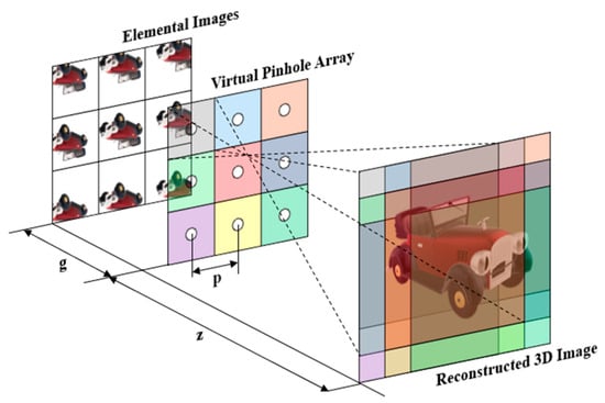
Figure 1.
Computational reconstruction method in integral imaging.
2.2. Existing Model for Scattering Medium with Spectral Analysis and Integral Imaging
A scattering model is derived from the relationship between a captured image, a scattering medium, and the original image without the scattering medium. It can be employed to reduce the scattering artifacts in the captured image. The standard model used in dehazing methods is derived from the Bouguer–Lambert–Beer law [,], as follows:
Here, g(x) represents the image captured by a camera, f(x) is the original image to be reconstructed, and the intensity of the ambient light is denoted by A. The medium transmission, denoted as t(x), is the weight function affecting the original image. It can be seen that determining the values of A and t(x) is important in order to reconstruct f(x) from g(x). However, this model makes it somewhat complicated to separate t(x)f(x), requiring a complicated dehazing algorithm []. Thus, a simpler model is introduced [], which is written as:
In Equation (2), g(x) is the image signal affected by the scattering medium, f(x) is the original signal unaffected by the scattering medium, and t(x) is the scattering medium. Here, α is the visibility factor. This model can be easily analyzed in the spectral domain since the model consists of a linear combination of f(x) and t(x). Thus, applying the linearity of Fourier transformation to Equation (2), we can easily obtain Equation (3) as follows.
where G(ω), F(ω), and T(ω) represent the Fourier-transformed signals of g(x), f(x), and t(x), respectively. By estimating T(ω) and α, we can obtain the reconstructed F(ω) from G(ω). We utilize the frequency characteristics of the scattering medium to predict T(ω).
The results presented in Figure 2e demonstrate that the influence of the scattering medium dominates the very-low-frequency components of the image. Therefore, by utilizing the frequency characteristics of the scattering medium, we can determine the low-frequency components of the observed signal G(ω) as the components of T(ω) and the high-frequency components as the components of F(ω). These are then represented by
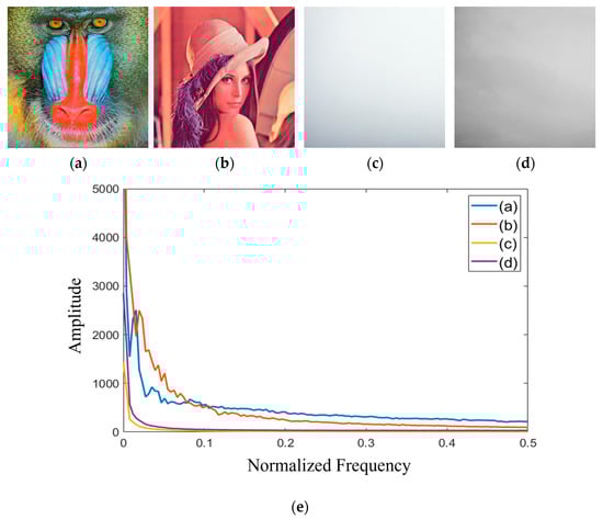
Figure 2.
(a) Baboon; (b) Lenna; (c) hazed image1; (d) hazed image2; (e) graph of spectrum for (a–d).
The spectrum-based method [] is illustrated in Figure 3. To estimate the effect of the scattering medium, fc is determined to separate lower-band and higher-band signals. The cut-off frequency fc is used for a low-pass filter to remove the effect of the scattering medium. The remaining high-frequency signal is then utilized to restore the high-frequency components of the original signal using the visibility coefficient α. The cut-off frequency fc is determined through Equation (6).
where GN(ω) is the normalized value of G(ω).
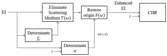
Figure 3.
Block diagram of a spectral-based method.
The visibility coefficient α is determined by applying the Beer–Lambert–Bouguer law. According to this law, the amount of transmitted light I(z) = I0·exp(−kz) is defined, where I0 is the amount of light from the original source and z is the distance from the sensor. Here, k denotes the total attenuation coefficient depending on the wavelength of the illumination and the medium. This coefficient primarily determines the amount of attenuation, absorption, and scattering of light within the scattered environment. Since visibility decreases due to the attenuation of the original signal, the total attenuation coefficient and the visibility coefficient α are related. Therefore, α can be rewritten as
The parameter k is related to the variance v of GN(ω) as
where . Here, k0 is a constant number which can be obtained experimentally.
3. Proposed Method
In this chapter, we discuss image enhancement of computational integral imaging via reducing the scattering artifact. A computational integral imaging reconstruction (CIIR) method can convert an elemental image array into a series of reconstructed images by adjusting the distance. These reconstructed images can suffer from blurring artifacts at out-of-focus locations. In particular, blurring artifacts from occluding objects can be scattered to the target object in reconstructed images. Thus, the reconstructed images for the target object can suffer from the scattering artifact from occluding objects, especially blurring or color changing. To enhance the reconstructed images, it is necessary to remove scattering artifacts caused by occlusion.
In the previous chapter, it can be observed that the visibility coefficient α is the most crucial factor in removing the scattering components of the image. Based on this, this paper presents a novel approach for estimating the visibility coefficient and applies it to the proposed computational integral imaging reconstruction method to improve image quality. The proposed method is depicted in Figure 4.
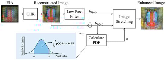
Figure 4.
Block diagram of the proposed method.
First, a reconstructed image is obtained from an EIA using the standard CIIR method. It is then separated into a low-band image and a high-band image using a low-pass filter. The visibility coefficient α is determined by using the probability density function (PDF) of the high-band image. The histogram of the band image is stretched using the parameter α, and the low and high bands are merged to obtain the enhanced image.
The process that demands the most computational time in our proposed algorithm is the low-pass filter, because the filter size is very large. Thus, we employ a moving average filter as the low-pass filter. As the size of the filter increases, the computational complexity also increases, so we introduce integral images for fast computation. The integral image [,] is an image that contains the sum of pixels up to the current position in the image. By using an integral image, we can quickly calculate the sum of a rectangular region in an image regardless of its size.
3.1. Formulations of Proposed Model
We derive a new formula using Equation (3) from the spectrum-based method []. In contrast to the existing method, we eliminate the complicated process of determining the cut-off frequency fc because a moving average filter is less sensitive to the cut-off frequency. We also introduce a new method for estimating α in our post-processing method, since the previous method of estimating α cannot be directly applied to a single image.
Figure 5 shows the spectra of G(ω), F(ω), and T(ω) images, assuming that only the low frequencies are present in T(ω), based on the results of Figure 2e.
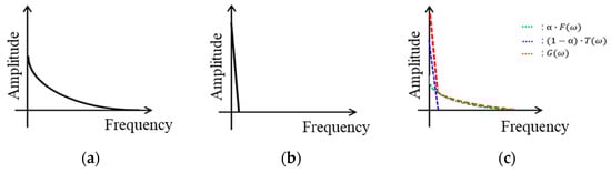
Figure 5.
The spectrum graphs: (a) F(ω); (b) T(ω); (c) G(ω).
In Figure 5, we can observe that the low-frequency components of G(ω) are greatly influenced by T(ω), while the high-frequency components of G(ω) are predominantly influenced by F(ω). These characteristics indicate that the low-frequency band Fl(ω) and the high-frequency band of F(ω) can be represented as
where Gl(ω) is the low-frequency band of G(ω) and Gh(ω) is the high-frequency band of G(ω). Since Tl(ω) and Fl(ω) cannot be directly determined in this model, Fl(ω) is estimated from Gl(ω) and the visibility coefficient α. Based on the analysis, our model suggests that the F(ω) of the original image, unaffected by the scattering medium, can be written as
3.2. Estimation of Visibility Coefficient
To estimate the visibility coefficient α in our model, we employ the probability density function (PDF) of the high-frequency band. Figure 6 shows the typical PDF of a high-frequency band of an image. In a general image unaffected by the scattering medium, the PDF of its high-frequency band exhibits a broad Gaussian shape, as shown in Figure 6b. However, in an image affected by the scattering medium, the presence of strong low-frequency components results in a narrower shape for the PDF of the high-frequency band. This is illustrated in Figure 6d. These characteristics can be utilized to approximate the PDF of the image affected by the scattering medium to that of the normal image. Thus, the coefficient α can be determined by a range ratio of two PDFs, which is written as
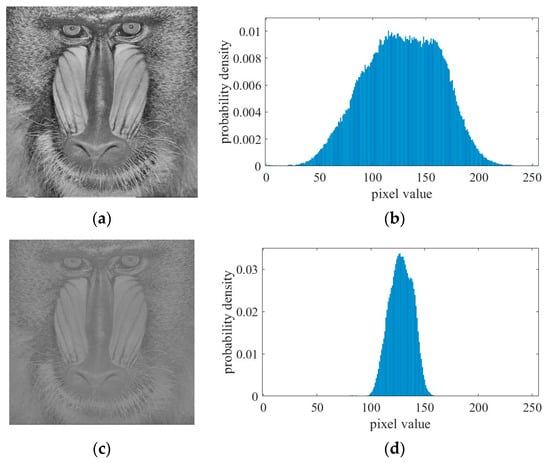
Figure 6.
Probability density function for high-band images: (a) high-band image of baboon; (b) PDF of (a); (c) high-band image of baboon with α-blending (α = 0.3); (d) PDF of (c).
In Equation (12), Gh(ω) is the high-frequency band image affected by the scattering medium and Fh(ω) is high-frequency band image of the original image. The coefficient α is determined by the ratio of the range of the probability density function of Gh(ω) to the range of the probability density function of Fh(ω). The range of the probability density function of Fh(ω) is experimentally determined with a value of 128. The range of the probability density function of Gh(ω) is defined as Equation (13), where p(x) represents the probability density function of Gh(ω). The range of p(x) is calculated by the point where a rate of 95% of the total number of pixels is populated. The reference rate is also determined experimentally. Once the coefficient α is determined, the proposed histogram stretching is performed using Equation (11). For example, illustrated in Figure 7 is the comparison of the two ranges of PDFs for the hazed image and the original image. And the proposed histogram stretching method can be effective for matching the two ranges.
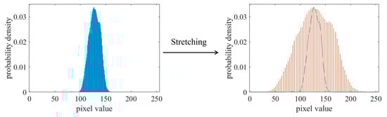
Figure 7.
Histogram stretching.
4. Experimental Results and Discussion
To evaluate the proposed algorithm, we conducted two experiments. First, we carried out an experiment with respect to visibility coefficient estimation. The objective of the first experiment was to evaluate the accuracy of the estimated visibility parameter. To achieve this, experimental images were generated from the original images and scattering medium images, as shown in Figure 8. Here, the experimental images ere generated based on the α-blending method using Equation (3), as illustrated in Figure 9. A total of 24 images were generated using Equation (3), with the visibility coefficients adjusted to 0.3, 0.5, and 0.7. The experiment compared the estimation of α using the previous method with that using the proposed method. And the size of the moving average filter was set to 131 × 131 for the proposed method.
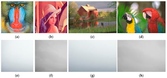
Figure 8.
Test dataset. (a) Baboon; (b) Lenna; (c) kodim22; (d) kodim23; (e) hazed image1; (f) hazed image2; (g) hazed image3; (h) hazed image4.
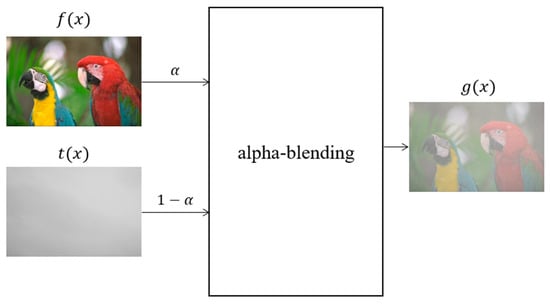
Figure 9.
Generating experimental images through alpha-blending.
Figure 10 shows some of the resulting images from the experiment, indicating that the quality of the reconstructed images improved subjectively. It can be observed that the resulting images obtained from the previous method with inaccurate visibility coefficients suffered from over-amplification in color. To quantitatively compare these results, we computed the peak signal-to-noise ratio (PSNR) and the structural similarity index measure (SSIM). Table 1 presents the visibility coefficients estimated by the proposed method and the previous method. The proposed method demonstrated more accurate estimated values for α, with averages of 0.32 for α = 0.3, 0.52 for α = 0.5, and 0.72 for α = 0.7, in comparison to the previous method. The PSNR results shown in Table 2 indicate that the proposed method yielded a PSNR improvement of 3.99 dB on average. Table 3 presents the results of the SSIM values between the original images and the resulting images. The SSIM results also demonstrate that the proposed method was superior to the previous method in terms of the improvement in image quality. This is because the visibility coefficients were accurately estimated by the proposed method with the spectral model. These results indicate that accurate estimation of the visibility coefficient plays an important role in improving image quality.
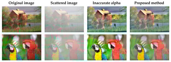
Figure 10.
Experimental results with visibility coefficient estimation.

Table 1.
Estimation results of visibility coefficient.
Table 2.
PSNR results with visibility coefficient estimation.
Table 3.
SSIM results with visibility coefficient estimation.
In addition, we carried out another experiment by applying the proposed method to CIIR. The objective of the second experiment was to evaluate the performance of the proposed CIIR method. Here, the proposed method was compared with two existing methods. As shown in Figure 11, EIAs were generated from original test images. Then, CIIR methods were used to convert the generated EIA into the reconstructed images. The sizes of the input images were either 512 × 512 or 768 × 512. The number of elemental images in EIA was 17 × 17, and each elemental image consisted of either 150 × 150 pixels or 300 × 300 pixels. The distances between the virtual pinhole array and the objects were z mm and 2z mm, respectively. Here, a moving average filter was employed as the low-pass filter, with a filter size of 131 × 131.
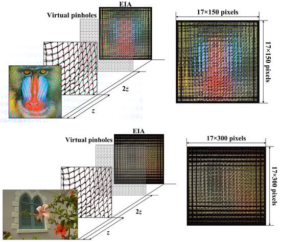
Figure 11.
Simulator for EIA generation.
Table 4 and Table 5 show the PSNR results and the SSIM results, respectively. The PSNR results reveal that the proposed method provided an average improvement of 1.45 dB over the standard CIIR method and 4.37 dB over the previous CIIR method. Furthermore, the SSIM results demonstrate the superiority of the proposed method over existing approaches. As depicted in Figure 12, the resulting images from the proposed method provided better performance in terms of subjective image quality compared with the standard CIIR method. Therefore, the proposed method achieved both objective and subjective improvements in the image quality of computational integral imaging systems.
Table 4.
PSNR results with CIIR methods.
Table 5.
SSIM results with CIIR methods.
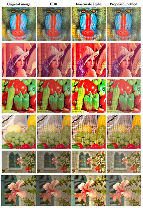
Figure 12.
Experimental results with CIIR methods.
5. Conclusions
We have presented an image enhancement method for computational integral imaging by introducing an efficient estimation technique for the visibility coefficient. Our method is based on a new spectral model for the scattering artifact. Unlike existing approaches that utilize a pre-processing method for elemental images before CIIR, our method employs a post-processing method for the reconstructed images after CIIR. The experimental results indicate that our approach enhances the image quality of computational integral imaging systems by eliminating scattering artifacts. Additionally, we introduced a novel method for estimating the visibility coefficient, a crucial parameter to eliminate scattering artifacts. The computer experiments indicated that our CIIR method was superior to the existing methods. Thus, we expect that the proposed method will be useful in improving the image quality of 3D computational integral imaging systems and image-dehazing systems [,,,,,,,,,,,].
Author Contributions
Conceptualization, H.Y.; methodology, H.C. and H.Y.; software, H.C. and H.Y.; validation, H.C. and H.Y.; formal analysis, H.Y.; investigation, H.C. and H.Y.; resources, H.Y.; data curation, H.C. and H.Y. writing—original draft preparation, H.Y.; writing—review and editing, H.C. and H.Y.; visualization, H.C.; supervision, H.Y.; project administration, H.Y. All authors have read and agreed to the published version of the manuscript.
Funding
This research was funded by a 2024 research grant from Sangmyung University.
Institutional Review Board Statement
Not applicable.
Informed Consent Statement
Not applicable.
Data Availability Statement
The raw data supporting the conclusions of this article will be made available by the authors on request.
Conflicts of Interest
The authors declare no conflicts of interest.
References
- Lippmann, G. Epreuves reversibles donnant la sensation du relief. J. Phys. Theor. Appl. 1908, 7, 821–825. [Google Scholar] [CrossRef]
- Javidi, B.; Carnicer, A.; Arai, J.; Fujii, T.; Hua, H.; Liao, H.; Martínez-Corral, M.; Pla, F.; Stern, A.; Waller, L.; et al. Roadmap on 3D integral imaging: Sensing, processing, and display. Opt. Express 2022, 28, 32266–32293. [Google Scholar] [CrossRef]
- Li, H.; Wang, S.; Zhao, Y.; Wei, J.; Piao, M. Large-scale elemental image array generation in integral imaging based on scale invariant feature transform and discrete viewpoint acquisition. Displays 2021, 69, 102025. [Google Scholar] [CrossRef]
- Jang, J.S.; Javidi, B. Three-dimensional synthetic aperture integral imaging. Opt. Express 2022, 27, 1144–1146. [Google Scholar] [CrossRef]
- Xing, S.; Sang, X.; Yu, X.; Duo, C.; Pang, B.; Gao, X.; Yang, S.; Guan, Y.; Yan, B.; Yuan, J.; et al. High-efficient computer-generated integral imaging based on the backward ray-tracing technique and optical reconstruction. Opt. Express 2017, 25, 330–338. [Google Scholar] [CrossRef] [PubMed]
- Xing, Y.; Wang, Q.H.; Ren, H.; Luo, L.; Deng, H.; Li, D.H. Optical arbitrary-depth refocusing for large-depth scene in integral imaging display based on reprojected parallax image. Opt. Commun. 2019, 433, 209–214. [Google Scholar] [CrossRef]
- Sang, X.; Gao, X.; Yu, X.; Xing, S.; Li, Y.; Wu, Y. Interactive floating full-parallax digital three-dimensional light-field display based on wavefront recomposing. Opt. Express 2018, 26, 8883–8889. [Google Scholar] [CrossRef] [PubMed]
- Wu, W.; Wang, S.; Zhong, C.; Piao, M.; Zhao, Y. Integral imaging with full parallax based on mini LED display unit. IEEE Access 2019, 7, 32030–32036. [Google Scholar] [CrossRef]
- Yanaka, K. Integral photography using hexagonal fly’s eye lens and fractional view. Proc. SPIE 2008, 6803, 533–540. [Google Scholar]
- Lee, E.; Cho, H.; Yoo, H. Computational Integral Imaging Reconstruction via Elemental Image Blending without Normalization. Sensors 2023, 23, 5468. [Google Scholar] [CrossRef]
- Lee, J.J.; Lee, B.G.; Yoo, H. Depth extraction of three-dimensional objects using block matching for slice images in synthetic aperture integral imaging. Appl. Opt. 2011, 50, 5624–5629. [Google Scholar] [CrossRef] [PubMed]
- Hong, S.H.; Jang, J.S.; Javidi, B. Three-dimensional volumetric object reconstruction using computational integral imaging. Opt. Express 2004, 12, 483–491. [Google Scholar] [CrossRef]
- Stern, A.; Javidi, B. Three-dimensional image sensing and reconstruction with time-division multiplexed computational integral imaging. Appl. Opt. 2003, 42, 7036–7042. [Google Scholar] [CrossRef]
- Shin, D.H.; Yoo, H. Image quality enhancement in 3D computational integral imaging by use of interpolation methods. Opt. Express 2007, 15, 12039–12049. [Google Scholar] [CrossRef] [PubMed]
- Shin, D.H.; Yoo, H. Computational integral imaging reconstruction method of 3D images using pixel-to-pixel mapping and image interpolation. Opt. Commun. 2009, 282, 2760–2767. [Google Scholar] [CrossRef]
- Cho, M.; Javidi, B. Computational reconstruction of three-dimensional integral imaging by rearrangement of elemental image pixels. J. Disp. Technol. 2009, 5, 61–65. [Google Scholar] [CrossRef]
- Inoue, K.; Cho, M. Visual quality enhancement of integral imaging by using pixel rearrangement technique with convolution operator (CPERTS). Opt. Lasers Eng. 2018, 111, 206–210. [Google Scholar] [CrossRef]
- Yang, C.; Wang, J.; Stern, A.; Gao, S.; Gurev, V.; Javidi, B. Three-dimensional super resolution reconstruction by integral imaging. J. Disp. Technol. 2015, 11, 947–952. [Google Scholar] [CrossRef]
- Yoo, H. Axially moving a lenslet array for high-resolution 3D images in computational integral imaging. Opt. Express 2013, 21, 8873–8878. [Google Scholar] [CrossRef]
- Yoo, H.; Jang, J.Y. Intermediate elemental image reconstruction for refocused three-dimensional images in integral imaging by convolution with δ-function sequences. Opt. Lasers Eng. 2017, 97, 93–99. [Google Scholar] [CrossRef]
- Yoo, H.; Shin, D.H. Improved analysis on the signal property of computational integral imaging system. Opt. Express 2007, 15, 14107–14114. [Google Scholar] [CrossRef] [PubMed]
- Yoo, H. Artifact analysis and image enhancement in three-dimensional computational integral imaging using smooth windowing technique. Opt. Lett. 2011, 36, 2107–2109. [Google Scholar] [CrossRef] [PubMed]
- Jang, J.Y.; Shin, D.; Kim, E.S. Improved 3-D image reconstruction using the convolution property of periodic functions in curved integral-imaging. Opt. Lasers Eng. 2014, 54, 14–20. [Google Scholar] [CrossRef]
- Jang, J.Y.; Shin, D.; Kim, E.S. Optical three-dimensional refocusing from elemental images based on a sifting property of the periodic δ-function array in integral-imaging. Opt. Express 2014, 22, 1533–1550. [Google Scholar] [CrossRef] [PubMed]
- Wu, W.; Wang, S.; Chen, W.; Qi, Z.; Zhao, Y.; Zhong, C.; Chen, Y. Computational Integral Imaging Reconstruction Based on Generative Adversarial Network Super-Resolution. Appl. Sci. 2024, 14, 656. [Google Scholar] [CrossRef]
- Yi, F.; Jeong, O.; Moon, I.; Javidi, B. Deep learning integral imaging for three-dimensional visualization, object detection, and segmentation. Opt. Lasers Eng. 2021, 146, 106695. [Google Scholar] [CrossRef]
- Aloni, D.; Yitzhaky, Y. Automatic 3D object localization and isolation using computational integral imaging. Appl. Opt. 2015, 54, 6717–6724. [Google Scholar] [CrossRef] [PubMed]
- Yi, F.; Lee, J.; Moon, I. Simultaneous reconstruction of multiple depth images without off-focus points in integral imaging using a graphics processing unit. Appl. Opt. 2014, 53, 2777–2786. [Google Scholar] [CrossRef] [PubMed]
- Kadosh, M.; Yitzhaky, Y. 3D Object Detection via 2D Segmentation-Based Computational Integral Imaging Applied to a Real Video. Sensors 2023, 23, 4191. [Google Scholar] [CrossRef]
- Zhang, M.; Piao, Y.; Kim, E.S. Visibility-enhanced reconstruction of three-dimensional objects under a heavily scattering medium through combined use of intermediate view reconstruction, multipixel extraction, and histogram equalization methods in the conventional integral imaging system. Appl. Opt. 2011, 50, 5369–5381. [Google Scholar]
- Cho, M.; Javidi, B. Three-dimensional visualization of objects in turbid water using integral imaging. J. Disp. Technol. 2010, 6, 544–547. [Google Scholar] [CrossRef]
- Markman, A.; Javidi, B. Learning in the dark: 3D integral imaging object recognition in very low illumination conditions using convolutional neural networks. OSA Contin. 2018, 1, 373–383. [Google Scholar] [CrossRef]
- Joshi, R.; Usmani, K.; Krishnan, G.; Blackmon, F.; Javidi, B. Underwater object detection and temporal signal detection in turbid water using 3D-integral imaging and deep learning. Opt. Express 2024, 32, 1789–1801. [Google Scholar] [CrossRef] [PubMed]
- Huang, Y.; Krishnan, G.; O’Connor, T.; Joshi, R.; Javidi, B. End-to-end integrated pipeline for underwater optical signal detection using 1D integral imaging capture with a convolutional neural network. Opt. Express 2023, 31, 1367–1385. [Google Scholar] [CrossRef] [PubMed]
- Usmani, K.; O’Connor, T.; Wani, P.; Javidi, B. 3D object detection through fog and occlusion: Passive integral imaging vs active (LiDAR) sensing. Opt. Express 2023, 31, 479–491. [Google Scholar] [CrossRef]
- Wani, P.; Usmani, K.; Krishnan, G.; O’Connor, T.; Javidi, B. Lowlight object recognition by deep learning with passive three-dimensional integral imaging in visible and long wave infrared wavelengths. Opt. Express 2022, 30, 1205–1218. [Google Scholar] [CrossRef] [PubMed]
- Shen, X.; Carnicer, A.; Javidi, B. Three-dimensional polarimetric integral imaging under low illumination conditions. Opt. Lett. 2019, 44, 3230–3233. [Google Scholar] [CrossRef]
- Lee, Y.; Yoo, H. Three-dimensional visualization of objects in scattering medium using integral imaging and spectral analysis. Opt. Lasers Eng. 2016, 77, 31–38. [Google Scholar] [CrossRef]
- Nayar, S.K.; Narasimhan, S.G. Vision in bad weather. In Proceedings of the Seventh IEEE International Conference on Computer Vision, Kerkyra, Greece, 20–27 September 1999; Volume 2, pp. 820–827. [Google Scholar]
- McCartney, E.J. Optics of the Atmosphere: Scattering by Molecules and Particles; John Wiley and Sons: New York, NY, USA, 1976. [Google Scholar]
- He, K.; Sun, J.; Tang, X. Single image haze removal using dark channel prior. IEEE Trans. Pattern Anal. Mach. Intell. 2010, 33, 2341–2353. [Google Scholar]
- Crow, F.C. Summed-area tables for texture mapping. In Proceedings of the 11th Annual Conference on Computer Graphics and Interactive Techniques, New York, NY, USA, 1 January 1984; pp. 207–212. [Google Scholar]
- Viola, P.; Jones, M.J. Robust real-time face detection. Int. J. Comput. Vis. 2004, 57, 137–154. [Google Scholar] [CrossRef]
- Guido, R.C.; Pedroso, F.; Contreras, R.C.; Rodrigues, L.C.; Guariglia, E.; Neto, J.S. Introducing the Discrete Path Transform (DPT) and its applications in signal analysis, artefact removal, and spoken word recognition. Digit. Signal Process. 2021, 117, 103158. [Google Scholar] [CrossRef]
- Guariglia, E.; Silvestrov, S. Fractional-Wavelet Analysis of Positive definite Distributions and Wavelets on D’(C). In Engineering Mathematics II; Springer: Cham, Switzerland, 2016; pp. 337–353. [Google Scholar]
- Yang, L.; Su, H.L.; Zhong, C.; Meng, Z.Q.; Luo, H.W.; Li, X.C.; Tang, Y.Y.; Lu, Y. Hyperspectral image classification using wavelet transform-based smooth ordering. Int. J. Wavelets Multiresolut. Inf. Process. 2019, 17, 1950050. [Google Scholar] [CrossRef]
- Guariglia, E. Harmonic Sierpinski Gasket and Applications. Entropy 2018, 20, 714. [Google Scholar] [CrossRef] [PubMed]
- Zheng, X.W.; Tang, Y.Y.; Zhou, J.T. A framework of adaptive multiscale wavelet decomposition for signals on undirected graphs. IEEE Trans. Signal Process. 2019, 67, 1696–1711. [Google Scholar] [CrossRef]
- Guariglia, E. Primality, Fractality and image analysis. Entropy 2019, 21, 304. [Google Scholar] [CrossRef] [PubMed]
- Berry, M.V.; Lewis, Z.V. On the Weierstrass-Mandelbrot fractal function. Proc. R. Soc. Lond. Ser. A 1980, 370, 459–484. [Google Scholar]
- Jeong, H.; Lee, E.; Yoo, H. Re-Calibration and Lens Array Area Detection for Accurate Extraction of Elemental Image Array in Three-Dimensional Integral Imaging. Appl. Sci. 2022, 12, 9252. [Google Scholar] [CrossRef]
- Li, X.; Yan, L.; Qi, P.; Zhang, L.; Goudail, F.; Liu, T.; Zhai, J.; Hu, H. Polarimetric imaging via deep learning: A review. Remote Sens. 2023, 15, 1540. [Google Scholar] [CrossRef]
- Tian, Z.; Qu, P.; Li, J.; Sun, Y.; Li, G.; Liang, Z.; Zhang, W. A Survey of Deep Learning-Based Low-Light Image Enhancement. Sensors 2023, 23, 7763. [Google Scholar] [CrossRef]
- Jakubec, M.; Lieskovská, E.; Bučko, B.; Zábovská, K. Comparison of CNN-based models for pothole detection in real-world adverse conditions: Overview and evaluation. Appl. Sci. 2023, 13, 5810. [Google Scholar] [CrossRef]
- Leng, C.; Liu, G. IFE-Net: An Integrated Feature Extraction Network for Single-Image Dehazing. Appl. Sci. 2023, 13, 12236. [Google Scholar] [CrossRef]
Disclaimer/Publisher’s Note: The statements, opinions and data contained in all publications are solely those of the individual author(s) and contributor(s) and not of MDPI and/or the editor(s). MDPI and/or the editor(s) disclaim responsibility for any injury to people or property resulting from any ideas, methods, instructions or products referred to in the content. |
© 2024 by the authors. Licensee MDPI, Basel, Switzerland. This article is an open access article distributed under the terms and conditions of the Creative Commons Attribution (CC BY) license (https://creativecommons.org/licenses/by/4.0/).