Virtual Sensor for Estimating the Strain-Hardening Rate of Austenitic Stainless Steels Using a Machine Learning Approach

Abstract

This study introduces a Multiple Linear Regression (MLR) model that functions as a virtual sensor for estimating the strain-hardening rate of austenitic stainless steels, represented by the Hardening Rate of Hot rolled and annealed Stainless steel sheet (HRHS) parameter. The model correlates tensile strength (Rm) with cold thickness reduction and chemical composition, evidencing a robust linear relationship with an R-coefficient above 0.9800 for most samples. Key variables influencing the HRHS value include Cr, Mo, Si, Ni, and Nb, with the MLR model achieving a correlation coefficient of 0.9983. The Leave-One-Out Cross-Validation confirms the model’s generalization for test examples, consistently yielding high R-values and low mean squared errors. Additionally, a simplified HRHS version is proposed for instances where complete chemical analyses are not feasible, offering a practical alternative with minimal error increase. The research demonstrates the potential of linear regression as a virtual sensor linking cold strain hardening to chemical composition, providing a cost-effective tool for assessing strain hardening behaviour across various austenitic grades. The HRHS parameter significantly aids in the understanding and optimization of steel behaviour during cold forming, offering valuable insights for the design of new steel grades and processing conditions.

1. Introduction

Austenitic Stainless Steels (ASS) exhibit high strain hardening during cold working processes such as rolling or forming, with mechanical properties improving as thickness is reduced [1]. Many austenitic grades are metastable at room temperature, which means that the austenitic phase is transformed into martensite during cold working; this is known as strain-induced martensite (SIM) [2]. The formation of martensite by SIM depends on the thermodynamic stability of the austenite and is influenced by the chemical composition, grain size, and forming parameters, including the amount of cold deformation, strain rate, and temperature, among others [3]. This mechanism of the transformation of austenite into martensite by SIM is mainly responsible for the strain hardening of ASS, and then, the superior work-hardening rate [4]. This is known as the transformation-induced plasticity (TRIP) effect and plays an important role in the final mechanical properties of ASS [1,2,5].

The M_d30 concept is extensively used to assess austenite stability in ASS, and it is influenced by the chemical composition and grain size. The parameter M_d30 predicts the temperature below which 50% of the austenitic microstructure transforms into martensite by SIM when the steel is tensile-strained to 30% elongation. Originally established through tensile testing, M_d30 is also widely applied in rolling deformation to estimate the austenite stability and, indirectly, the expected strain hardening [6]. A higher M_d30 temperature signifies lower austenite stability, leading to an increase in cold strain hardening due to greater martensite formation by SIM. Nohara et al. [7] proposed one of the most widely used expressions to estimate M_d30, shown in Equation (1):

$$M_{d30}\left(℃\right)=551-462·\left(C+N\right)-9.2·Si-8.1·Mn-13.7·Cr-29·\left(Ni+Cu\right)-18.5·Mo-68·Nb-1.42·\left(GS-8\right)$$

(1)

where M_d30 represents the temperature of the martensite formation induced by cold deformation and is expressed in °C. GS stands for grain size, measured according to the standard ASTM E91. Additionally, each alloying element is included in the equation with its chemical symbol and unit of weight percentage (%).

Various alternative expressions have been proposed for estimating M_d30, each placing different emphasis on the impact of chemical composition elements [8]. Nohara et al. take into account the combined effect of C and N, while Sjöberg considers the independent effects of C and N, suggesting that nitrogen is a more effective alloying element than carbon in restraining the transformation of austenite into martensite by SIM [9,10]. However, Masumura et al.’s recent work [11] demonstrates that the difference in the austenite-stabilizing effects of C and N grows as the temperature increases, owing to the difference in stacking fault energy between C- and N-added steels. They also found that the relation between M_d30 and C and N concentration is not linear, as previously assumed in other studies. The various expressions proposed to determine M_d30 aim to accurately predict this temperature, but it remains challenging to define experimentally. Despite the importance of understanding the transformation of austenite into martensite by SIM in metastable ASS for the forming industry, M_d30 should not be considered an exact measure of austenitic stability or an indicator of the hardening behaviour, but rather an approximation.

While the TRIP effect is the most relevant one in the hardening of ASS, other mechanisms also contribute to increasing their main mechanical properties [12], such as grain refinement by recrystallization [13], an increase in δ ferrite content [14], and solid solution strengthening [13,14]. Mechanical testing is commonly used to quantitatively analyse the combined effect of all these different hardening mechanisms. The two most widely used tools are the strain-hardening exponent n, determined from the engineering stress–strain flow curve obtained from tensile tests [15], and the cold-rolling curves, which plot the evolution of the mechanical properties against the thickness reduction [16,17].

During the last decade, multiple works have been published, supporting the modelling of these mechanical parameters for several traditional ASS. One of the most extensively modelled aspects is the cold-strain-hardening behaviour of the AISI 304 austenitic. Several studies have reported nonlinear stress–strain models under various testing conditions; Arrayago et al. [15] proposed a revised predictive equation for the strain-hardening parameter n for the AISI 304 based on the Rasmussen model, while Fernando et al. [18] designed a new stress–strain model to accurately predict both tensile and compressive full-range stress–strain curves for the AISI 304. Furthermore, Jia et al. [19] established eight constitutive relations to predict the flow stress curves of the AISI 304 under different conditions of strain-hardening rate and temperature. In addition to these studies, Wang et al. [20] modelled the relationship between cold deformation and the mechanical properties of austenitic AISI 316L, combining theoretical analysis, numerical simulation and experimental uniaxial tensile testing. Moreover, Janeiro et al. [21] established a linear correlation between austenite deformation and martensite transformation for low-Ni ASS. The model predicts the stress–strain curve from the parameter M_s; this describes the initial temperature of the martensitic transformation and is related to the austenite stability. The majority of these studies demonstrate the distinct stages of strain-hardening behaviour in ASS, as evidenced by the stress–strain curves. The plastic deformation in these steels is greatly influenced by the microstructural phase transformation, which is the primary challenge in accurately modelling strain-hardening behaviour. Consequently, developing a single model to describe strain-hardening behaviour across a wide range of ASS becomes extremely difficult [22]. To address the complexity of simulating the strain-hardening behaviour of ASS, cold-rolling curves offer an accepted solution for estimating the strain-hardening rate by correlating the tensile strength (Rm) of steel with different cold-rolling deformations and the cold thickness reductions applied. This approach, as proposed by Su-Fen et al. for low-carbon steel [16], involves fitting the relationship between Rm with several cold-rolling and respective deformations to a second-degree polynomial equation, and then, using the Hollomon procedure to determine the strain-hardening exponent n. This is achieved by determining the slope of the linear relation between the logarithm of Rm and the logarithm of cold thickness reduction for the cold-rolled low-carbon steel.

In the field of ASS, several authors have reported experimental cold-rolling curves such as AISI 304 [23], 304L [24], 316 [25], and 201 [26,27] showing different evolutions of the mechanical properties and microstructure against the cold thickness reduction, depending on the steel grade. Various works have confirmed the effect of the chemical composition on mechanical behaviour. Di Schino et al. [14] confirmed the classical relationship of the Rm and Rp_0.2 with the solute concentration for the AISI 304 proposed by Pickering et al. [28], and Contreras et al. [29] demonstrated a linear relationship of the mechanical properties with the chemical composition and the cold thickness reduction for stainless steels. Therefore, determining the strain-hardening rate of a specific ASS requires experimental analysis. However, this process is both costly and time-consuming, estimated at 49 man hours per sheet of each ASS, and also requests physical samples, the availability of which can be limited, especially for newly designed materials or those under development. Then, the use of regression models is proposed as an economical and faster way of conducting such studies [30].

More recently, the concept of virtual sensors has been introduced in the industrial sector as a potential solution to reduce the risk of high-impact failures by improving detectability and predicting failure modes [31]. Examples of this technological advancement are the works of Nimo et al. [32], who developed a virtual sensor to replace a semi-manual procedure of the verification of the final chemical composition of stainless steels, and Abdolmohammadi et al. [33], who designed a model for geometry prediction after cold strain based on the virtual sensor for robotic sheet metal forming.

Stainless steel sheets are commonly subjected to forming processes to achieve the final product shape. During these processes, the steel undergoes cold strain hardening. The strain state and the strain-hardening rate are critical factors that influence the success of the sheet deformation process. Thus, from a manufacturing standpoint, it is very beneficial to develop a mathematical model to estimate the strain-hardening rate across a broad spectrum of ASS. Such a model would enable the prediction of the material behaviour prior to forming, thereby facilitating an assessment of its cold workability.

This paper aims to develop a new parameter for estimating the strain-hardening rate of traditional and new-generation ASS, which are used for applications such as in the food industry, drawing, furnaces, or decoration elements, among others. This development is based on the results obtained from a multiple linear regression (MLR) analysis, correlating $Rm$ with chemical composition and thickness reduction [29]. To accomplish this, a wide selection of ASS underwent cold rolling at the laboratory scale, encompassing various thickness reductions, followed by uniaxial tensile testing to obtain experimental cold-rolling curves. A database is compiled from these curves, facilitating the establishment of a linear regression (LR) model that expresses Rm as a function of the cold thickness reduction for each austenitic grade. Subsequently, based on the Hollomon procedure which defines the strain-hardening exponent n as the slope of the linear relation between the logarithm of stress and the logarithm of strain, and referencing the work of Su-Fen et al. [16] for low carbon steel, the slope of each linear relation between Rm and the cold thickness reduction is determined and defined as the strain-hardening rate of each ASS grade. Finally, these slopes are denoted as coefficient a and correlated with the chemical composition through MLR, culminating in the formulation of the new strain-hardening rate parameter designated as HRHS (Hardening Rate of Hot rolled and annealed Stainless steel sheet). This parameter can serve as a virtual sensor for the design and development of new ASS grades, as well as for optimizing cold-forming processes.

2. Materials and Methods

2.1. Materials

Several ASS grades were selected to cover a broad range of chemical compositions. Samples were obtained from industrial sheets with a thickness between 3.0 and 5.0 mm, following hot-rolling and intermediate annealing stages, corresponding to 1D mill finishing as per European Standard EN-10088-2 [34]. The number of collected samples was between one and five, depending on the industrial availability of each selected ASS. The average chemical compositions of the analysed steel grades are summarised in

Table 1. Identification and chemical composition, by weight percentage (wt %), of the selected industrial hot-rolled and annealed sheets. Grades without a standard designation are referred to by their internal Acerinox ID (in brackets) [35].

ID.	AISI [36]	EN [34]	C	Si	Mn	Cr	Ni	Cu	Mo	N	Nb	Ti	S
A1	301	1.4310	0.105	0.86	1.24	16.78	6.71	0.20	0.34	0.069	0.013	0.008	0.0010
A2	304	1.4301	0.029	0.38	1.75	17.89	8.06	0.42	0.25	0.074	0.011	0.010	0.0010
A3	316L	1.4404	0.022	0.35	1.38	16.70	10.28	0.32	2.26	0.053	0.021	0.009	0.0020
A4	(ACX 041)	-	0.083	0.43	9.62	15.95	1.46	0.19	0.03	0.160	0.005	0.019	0.0020
A5	310S	1.4845	0.045	0.55	1.36	24.60	19.15	0.18	0.01	0.025	0.011	0.003	0.0010
A6	201	1.4372	0.076	0.50	7.06	16.12	4.32	0.58	0.18	0.083	0.008	0.004	0.0010
A7	904L	1.4539	0.019	0.42	1.50	19.58	24.52	1.40	4.25	0.015	0.022	0.006	0.0010
A8	309S	1.4833	0.044	0.49	1.63	22.37	13.94	0.28	0.49	0.058	0.007	0.013	0.0010

.

This selection covers a range of austenitic grades, starting from high-alloyed AISI 310S/EN 1.4845, AISI 309S/EN 1.4833, and AISI 904L/EN 1.4539, which have a high content of Cr, Ni, Mo, and/or Cu. These grades are designed to increase mechanical behaviour, corrosion resistance, and oxidation at high temperatures for applications such as furnaces, electrical resistances, high temperatures, refractories and tubes. On the other end of the spectrum are low Ni-austenitics such as AISI 201/EN 1.4372 and ACX 041. These grades contain higher Mn levels to substitute Ni, ensuring the stability of austenite during cold forming. Their mechanical properties and corrosion resistance are lower, but enough for their use in decoration and households. Additionally, the study includes the standard AISI 304/EN 1.4301 grade, with a medium content of Ni and Cr being extensively used in the food industry, tableware, household items and drawing applications. Other grades considered are the medium-alloyed austenitic AISI 301/EN 1.4310 steel, with higher C to increase the strength for applications like architectural and automotive elements, and the AISI 316L/EN 1.4404 type with higher Ni and Mo content to improve corrosion resistance, making it suitable for the chemical industry.

Initially, longitudinal strips are cut from each industrial sheet and cold-rolled in a Norton duo mill at a laboratory scale, applying thickness reductions ranging from 10% to 70%. Subsequently, the cold-rolled strips undergo machining and tensile testing according to ASTM E8/E8M standards. The engineering stress–strain flow curves for each steel grade are obtained, as illustrated in Figure 1a for the sample A2, and mechanical parameters, maximum tensile strength ($Rm$), yield strength at 0.2% strain (Rp_0.2), and elongation (A₅₀), are calculated.

2.2. Methods

2.2.1. Multiple Linear Regression

Next, the values of Rm obtained for each thickness reduction in every steel grade are plotted versus the thickness reduction to obtain the cold-rolling curves, as shown in Figure 1b. These curves are fitted using LR, and then the slope of each curve (coefficient a) is evaluated as an indicator of the strain-hardening rate for each steel grade. This slope is used as the output variable in the subsequent model to obtain the new parameter HRHS through regression.

The LR is expressed by Equation (2):

$$Rm=a·x+b$$

(2)

where $b$ is the ordinate–intercept when x is equal 0, a is the slope of the line of the $LR$, x is the independent variable (red, cold thickness reduction), and Rm is the dependent variable.

While the MLR is expressed by Equation (3):

$$HRHS=\sum w_i·x_i+c$$

(3)

where $c$ is the ordinate–intercept of the hyperplane $w_i·x_i$, $w_i$ are the estimated coefficients of the MLR model, $x_i$ are the independent variables (concentration of alloying elements), and HRHS is the dependent variable. Matrix $w_i$ values are estimated using the well-known least squares method with the training set of data.

Therefore, the LR is the result of an experimental test battery which offers the estimation of the slope of each Rm curve of the several ASS that have been considered in the work. Meanwhile, the MLR gives an approximation of this slope (coefficient a) from the chemical composition through the parameter HRHS for modified or new ASS grades without the need for additional tests. So, this MLR model acts as a virtual sensor of the strain-hardening rate of the material.

Finally, a database is constructed using the coefficients a (slopes of the Rm–cold thickness reduction curves obtained from LR) and the content of the alloying elements in each austenitic steel grade to develop a multiple linear regression model that correlates the strain-hardening rate with the chemical composition for the ASS family. The number of independent variables considered in this database is eleven, as described in

Table 2. Identification of variables used for both LR and MLR models.

Model	Variables	Symbol	Description (Units)
LR	Input	red	Cold thickness reduction (%)
	Output	Rm	Tensile Strength (MPa)
MLR	Input	Ni, Cr, Cu, Mn, Mo, Si, C, N, S, Ti, and Nb	Concentration of each alloying element (%)
	Output	HRHS	Theoretical hardening rate of a hot rolled and annealed stainless steel sheet (dimensionless)

.

The LR database consists of 123 samples, representing combinations of different cold thickness reductions ranging from 0% to 70% for 19 sheets of 8 ASS grades. For MLR, the database comprises 19 cases, each corresponding to the coefficient a for one of the 19 sheets used in LR.

2.2.2. Leave-One-Out Cross-Validation

Due to the relatively small size of the MLR database used to establish correlations between the hardening rate and chemical composition across the entire ASS family, it is necessary to apply a method to validate the new parameter HRHS. For this purpose, the Leave-One-Out Cross-Validation (LOOCV) method has been identified as extensively used [37,38,39,40,41]. Building on the research by [42], which was validated by LOOCV, this study uses process parameter maps for AISI 316L-Cu parts produced by selective laser melting to predict suitable parameters for different compositions, revealing nonlinear dependencies and highlighting process–property relationships. In [43], a dataset of 116 data points was analysed using the RFECV-LOO method to identify key parameters for ML models. Various ML models were evaluated using metrics like root mean squared error (RMSE), mean squared error (MSE), and correlation coefficient (R). Support vector regression (SVR) showed the highest accuracy, while lasso regression was the least effective. The models’ performance was validated through sensitivity and parametric analyses.

Given the database ${\left\{\left(x_i,y_i\right)\right\}}_{i=1}^n$, where $x_i$ are the inputs features and $y_i$ are the corresponding labels, from each $i$ from 1 to $n$. Remove the i-th data point, resulting in the training set $\left\{\left(x_j,y_j\right):j\ne i\right\}$. Train the model on this reduced training set to obtain the model eliminating the i-th data point ${\widehat{f}}^{-i}$ and use this trained model to predict the value for the left-out observation $x_i$, yielding the prediction ${\widehat{y}}_i={\widehat{f}}^{-i}\left(x_i\right)$. Equations (4) and (5) provide the mathematical foundation of the process. Equation (4) calculates the prediction error for each left-out observation.

$$e_i=y_i-{\widehat{y}}_i$$

(4)

Equation (5) shows the MSE:

$${MSE}_{LOO}=\frac{1}{n}{\sum }_{i=1}^n{\left(y_i-{\widehat{y}}_i\right)}^2$$

(5)

LOOCV involves training and testing models in all the possible ways of dividing the original sample into training and validation sets. In this study, the validation set consists of one observation, and the training set comprises 18 out of the 19 cases from the MLR database. With each pass, the observation data are rotated, resulting in a total of 19 models trained and tested using the LOOCV method, as described in

Table 3. Cross-validation strategy for the LOOCV procedure. The use of background color in the table serves the purpose of indicating the samples used for validating each model.

Steel Grade		A1			A2					A3			A4		A5		A6		A7	A8
# Sample		1	2	3	1	2	3	4	5	1	2	3	1	2	1	2	1	2	1	1
# model	LOO-1
	LOO-2
	LOO-3
	…
	LOO-19

.

3. Results

The results of the LR models, which establish the linear relationship between $Rm$ and the cold thickness reduction for each analysed steel sample, are shown in Figure 2. This includes the coefficient a in Figure 2a, representing quantitatively the slope of each regression line and serving as a dependent variable in the MLR model pursued in this work, as well as the values of R in Figure 2b. A higher R value indicates a better linear fit of the regression line between Rm and cold thickness reduction. The minimum R-value determined for the LR models is 0.9850 and maximum one is 0.9999.

The MLR model used to define the new parameter HRHS, which represents the strain-hardening rate of hot-rolled and annealed ASS sheets as a function of the chemical composition uses the coefficients a obtained from the LR models as the output variable and the chemical composition as the input variables. The Sum of Squares (SOS) [44], RMSE, MSE and R are some of the most extensively mathematical parameters used to measure the quality of an MLR model. This study employs the R and MSE as quality indices, resulting in values of 0.9983 and 0.0307, respectively. The expression for the HRHS parameter obtained by the MLR model is shown in Equation (6). The obtained results are displayed in Figure 3.

$$\begin{gathered} HRHS=33.560-5.046·C-1.473·Cr-0.389·Cu+0.195·Mn-2.406·Mo+8.044·N+ \\ 6.935·Si+0.446·Ni+133.524·S-41.093·Nb-27.245·Ti \end{gathered}$$

(6)

where HRHS is an estimated value of the strain-hardening rate for ASS, expressed in dimensionless form, and each alloying element is included in the equation with its chemical symbol and unit of weight percentage (%).

Figure 3a illustrates the outcomes of the MLR model for the HRHS parameter. The x-axis categorizes each analysed sample, with the initial two digits specifying the ASS grade and the subsequent one denoting the sheet number within that steel type. The primary y-axis quantifies the coefficient a values derived from individual LR models, represented by blue circles. In contrast, the secondary y-axis displays the HRHS values predicted by the MLR model across all austenitic grades, depicted as orange crosses. A tighter convergence of the crosses and circles signifies a better fit of the MLR model in predicting the HRHS parameter, as evidenced by higher correlation coefficients and diminished MSE. To discern the most impactful variables within the model, an evaluation of the p-values corresponding to the alloying elements is undertaken. The findings of this analysis are portrayed in Figure 3b, highlighting the alloying elements with the most significant influence on the HRHS estimation.

To validate the HRHS parameter’s formulation, the LOOCV method is employed as per the protocol outlined in Table 3. The results obtained from this validation procedure are illustrated in Figure 4. Specifically, Figure 4a plots the identification of each LOOCV model along the x-axis. The primary y-axis displays the coefficient a values obtained from the LR model for each sample, symbolized by blue circles. Concurrently, the secondary y-axis shows the corresponding HRHS estimates for the same sample when used as validation data in the LOOCV strategy, represented by orange crosses. A graphical representation of the R and MSE for each LOOCV model is presented in Figure 4b, plotted against the primary and secondary y-axes, respectively.

The MLR model is recalculated considering only the most significant variables determined by analysing the p-values from the initial MLR model. The contents of Cr, Mo, Si, Ni, and Nb are used as independent variables for the new MLR model, as shown in Equation (7), and the parameter is renamed as HRHS_simplified

$${HRHS}_{simplified}=35.01-1.429·Cr-2.381·Mo+5.538·Si+0.362·Ni-55.179·Nb$$

(7)

where HRHS_simplified, expressed in a dimensionless form, is an estimated value of the strain-hardening rate for ASS based on the most significant alloying elements. Each one of these chemical elements is expressed in weight percentage (%) and included in the equation with its respective chemical symbols.

The HRHS values predicted by the new simplified expression for each analysed ASS are plotted in Figure 5 against the correspondent coefficients a obtained from the LR models.

4. Discussion

The yield strengths, Rp_0.2 and Rp_1.0, and also the tensile strength, Rm, are mechanical parameters normally used for the comparison of the hardening level of materials in the industrial design sector for applications that request cold-forming operations. In this work, the mechanical parameter Rm is chosen as an indicator of this strain-hardening rate, and the relationship between this property and the degree of thickness reduction by cold rolling is established by LR for each ASS grade under study. The values of the coefficient a ranging between 7.2 and 17.2 with good repeatability between the different analysed samples for the same steel grade (see Figure 2a). The high values of R in Figure 2b, greater than 0.9850, confirm the good linear relationship between Rm and cold thickness reduction for the analysed austenitic grades. Therefore, it can be concluded that the coefficient a is influenced by the steel grade, i.e., the chemical composition.

This coefficient a is used as the dependent variable in an MLR model to predict the strain-hardening rate as a function of the chemical composition. The output variable of this model is the proposed HRHS parameter which is calculated by the model as a function of the main alloying elements, rather than being experimentally determined from the cold-rolling curves. Equation (6) derived from this MLR model, revealing the effect of the 11 alloying elements (C, Si, Mn, Cr, Ni, Cu, Mo, N, Nb, Ti and S). The model’s goodness fit is indicated by the R value of 0.9983 and MSE of 0.0307, both of which confirm the good accuracy of the new HRHS parameter. This is supported by Figure 3a, which shows the close alignment between the coefficients a obtained from each LR model and the HRHS value derived from the MLR model.

The analysis of the p-values associated with each alloying element of the MLR model identifies that Cr, Mo, Si, Ni and Nb are the most significant independent variables. This means that they carry the greatest weight in the estimation of the HRHS value. A p-value lower than 0.05 for these alloying elements is reported by Figure 3b, confirming their significance. Subsequently, a new MLR model is tested with only these significant independent variables, providing a new version of the HRHS parameter, referred to as HRHS_simplified defined by Equation (7). This approach allows for estimating the cold hardening rate with fewer chemical elements, without the need for a more complete chemical composition analysis of a steel grade, and yields good results in fitting the new MLR model. Figure 5 shows a good agreement between the coefficients a obtained from each LR model and the HRHS_simplified estimations derived from the new MLR model; both parameters are closely aligned. Additionally, the R and MSE values (0.9925 and 0.1353, respectively) are rather close to the ones obtained in the MLR model of the HRHS parameter.

Finally, the HRHS model is validated using the LOOCV strategy, which involves splitting the original sample into training and validation sets. The results shown in Figure 4a confirm the good fit between the coefficient a obtained for each sample from the LR model and the corresponding HRHS estimated with the LOOCV model using the same sample as the validation data. The values of R and MSE for each LOOCV model shown in Figure 4b also validate the MLR model, with the R coefficient being greater than 0.9980 and the MSE values lower than 0.0318 for all LOOCV models.

5. Conclusions

Based on the observed relationship between the mechanical properties, chemical composition, and cold thickness reduction for the ASS grades under hardening conditions in previous research [29], a new multiple linear regression (MLR) approach is designed to predict the strain-hardening rate of ASS as a function of their chemical composition. The main conclusions drawn from this work are as follows:

• The strain-hardening rate of each ASS grade can be accurately predicted (R coefficient exceeding 0.9800 for all analysed samples, except in three cases), due to the observed linearity between Rm and the cold thickness reduction;
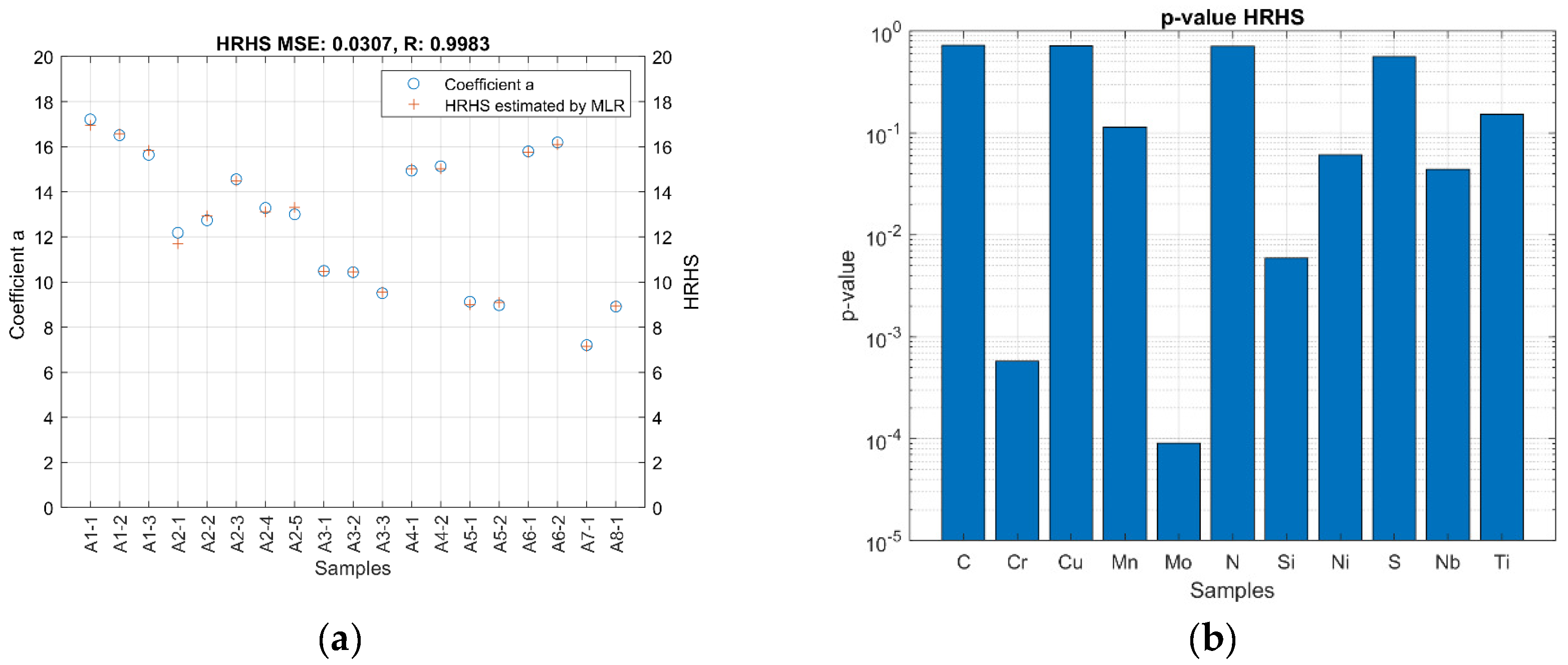
• A strong linear correlation exists between individual hardening rate values and the chemical composition across the entire austenitic family, encapsulated by a single parameter known as the HRHS (standing from Hardening Rate of Hot rolled and annealed Stainless steel sheet) coefficient; the MLR indicates a correlation of 0.9983;
• The analysis of the most significant variables in the MLR model indicates that Cr, Mo, Si, Ni, and Nb are the independent variables contributing most to estimating the HRHS value;
• Validation of the HRHS parameter is confirmed through the LOOCV strategy, with consistently high R values and low MSE across various models using different samples for validation. The correlation coefficients often exceed 0.9980 and the MSE values are lower than 0.0318;
• A simplified form of the HRHS parameter is proposed, which can be used as a practical alternative when it is not feasible to obtain chemical analyses of all alloying elements; the HRHS_simplified parameter yields acceptable results with only a modest increase in expected error.

This study demonstrates that linear regression techniques can establish good correlations between the cold strain hardening and the chemical composition of ASS. It confirms the potential of these methods for modelling the mechanical behaviour of steels.

The newly developed HRHS parameter provides a simple and cost-effective way to compare the impact of various chemical compositions on strain-hardening behaviour across different austenitic grades under the same process conditions (such as strain-hardening rate, strain level, and temperature). Therefore, the significance of the HRHS parameter lies in its ability to enhance the understanding of how a new austenitic steel behaves during cold forming compared to traditional varieties. This is considered as a virtual sensor for designing new steel grades or optimizing current and future processing conditions.

References

1. Sohrabi, M.J.; Naghizadeh, M.; Mirzadeh, H. Deformation-induced martensite in austenitic stainless steels: A review. In Archives of Civil and Mechanical Engineering; Springer Science and Business Media: Berlin/Heidelberg, Germany, 2020; Volume 20. [Google Scholar] [CrossRef]
2. Järvenpää, A.; Jaskari, M.; Kisko, A.; Karjalainen, P. Processing and Properties of Reversion-Treated Austenitic Stainless Steels. Metals 2020, 10, 281. [Google Scholar] [CrossRef]
3. Lo, K.H.; Shek, C.H.; Lai, J.K.L. Recent developments in stainless steels. Mater. Sci. Eng. R Rep. 2009, 65, 39–104. [Google Scholar] [CrossRef]
4. Padilha, A.F.; Plaut, R.L.; Rios, P.R. Annealing of cold-worked austenitic stainless steels. ISIJ Int. 2003, 43, 135–143. [Google Scholar] [CrossRef]
5. Karjalainen, L.P.; Taulavuori, T.; Sellman, M.; Kyröläinen, A. Some strengthening methods for austenitic stainless steels. Steel Res. Int. 2008, 79, 404–412. [Google Scholar] [CrossRef]
6. Angel, T. Formation of martensite in austenitic stainless steels. J. Iron Steel Inst. 1954, 177, 165–174. [Google Scholar]
7. Nohara, K.; Ono, Y.; Ohashi, N. Composition and Grain Size Dependencies of Strain-Induced Martensitic Transformation in Metastable Austenitic Stainless Steels. Tetsu-to-Hagané 1977, 63, 772–782. [Google Scholar] [CrossRef]
8. Kirsch, B.; Hotz, H.; Müller, R.; Becker, S.; Boemke, A.; Smaga, M.; Beck, T.; Aurich, J.C. Generation of deformation-induced martensite when cryogenic turning various batches of the metastable austenitic steel AISI 347. Prod. Eng. 2019, 13, 343–350. [Google Scholar] [CrossRef]
9. Sjöberg, J. Influence of analysis on the properties of stainless spring steel. Wire 1973, 23, 155–158. [Google Scholar]
10. Jeon, J.B.; Chang, Y.W. Effect of nitrogen on deformation-induced martensitic transformation in an austenitic 301 stainless steels. Metals 2017, 7, 503. [Google Scholar] [CrossRef]
11. Masumura, T.; Fujino, K.; Tsuchiyama, T.; Takaki, S.; Kimura, K. Effect of carbon and nitrogen on Md30 in metastable austenitic stainless steel. ISIJ Int. 2021, 61, 546–555. [Google Scholar] [CrossRef]
12. Mirzaie, T.; Mirzadeh, H.; Naghizadeh, M. Contribution of different hardening mechanisms during cold working of AISI 304L austenitic stainless steel. Arch. Metall. Mater. 2018, 63, 1317–1320. [Google Scholar] [CrossRef] [PubMed]
13. Järvenpää, A.; Jaskari, M.; Juuti, T.; Karjalainen, P. Demonstrating the effect of precipitation on the mechanical stability of fine-grained austenite in reversion-treated 301LN stainless steel. Metals 2017, 7, 344. [Google Scholar] [CrossRef]
14. Di Schino, A.; Richetta, M. Evaluation of the metallurgical parameters effect on tensile properties in austenitic stainless steels. Acta Metall. Slovaca 2017, 23, 111–121. [Google Scholar] [CrossRef]
15. Arrayago, I.; Real, E.; Gardner, L. Description of stress-strain curves for stainless steel alloys. Mater. Des. 2015, 87, 540–552. [Google Scholar] [CrossRef]
16. Su-Fen, W.; Yan, P.; Zhi-Jie, L. Work-hardening and deformation mechanism of cold rolled low carbon steel. Res. J. Appl. Sci. Eng. Technol. 2013, 5, 823–828. [Google Scholar] [CrossRef]
17. Bhav Singh, B.; Sivakumar, K.; Balakrishna Bhat, T. Effect of cold rolling on mechanical properties and ballistic performance of nitrogen-alloyed austenitic steels. Int. J. Impact Eng. 2009, 36, 611–620. [Google Scholar] [CrossRef]
18. Fernando, D.; Teng, J.G.; Quach, W.M.; De Waal, L. Full-range stress-strain model for stainless steel alloys. J. Constr. Steel Res. 2020, 173, 106266. [Google Scholar] [CrossRef]
19. Jia, B.; Zhang, Y.; Rusinek, A.; Xiao, X.; Chai, R.; Gu, G. Thermo-viscoplastic behavior and constitutive relations for 304 austenitic stainless steel over a wide range of strain rates covering quasi-static, medium, high and very high regimes. Int. J. Impact Eng. 2022, 164, 104208. [Google Scholar] [CrossRef]
20. Wang, S.; Xue, H.; Cui, Y.; Tang, W.; Gong, X. Effect of Different Cold Working Plastic Hardening on Mechanical Properties of 316L Austenitic Stainless Steel. Procedia Struct. Integr. 2018, 13, 1940–1946. [Google Scholar] [CrossRef]
21. Janeiro, I.; Hubert, O.; Schmitt, J.H. In-situ strain induced martensitic transformation measurement and consequences for the modeling of medium Mn stainless steels mechanical behavior. Int. J. Plast. 2022, 154, 103248. [Google Scholar] [CrossRef]
22. Li, T.; Zheng, J.; Chen, Z. Description of full-range strain hardening behavior of steels. SpringerPlus 2016, 5, 1316. [Google Scholar] [CrossRef] [PubMed]
23. Milad, M.; Zreiba, N.; Elhalouani, F.; Baradai, C. The effect of cold work on structure and properties of AISI 304 stainless steel. J. Mater. Process. Technol. 2008, 203, 80–85. [Google Scholar] [CrossRef]
24. Hedayati, A.; Najafizadeh, A.; Kermanpur, A.; Forouzan, F. The effect of cold rolling regime on microstructure and mechanical properties of AISI 304L stainless steel. J. Mater. Process. Technol. 2010, 210, 1017–1022. [Google Scholar] [CrossRef]
25. Mahmoudiniya, M.; Kheirandish, S.; Asadiasadabad, M. The Effect of Cold Rolling on Microstructure and Mechanical Properties of a New Cr–Mn Austenitic Stainless Steel in Comparison with AISI 316 Stainless Steel. Trans. Indian Inst. Met. 2017, 70, 1251–1259. [Google Scholar] [CrossRef]
26. Souza Filho, I.R.; Sandim, M.J.R.; Cohen, R.; Nagamine, L.C.C.M.; Hoffmann, J.; Bolmaro, R.E.; Sandim, H.R.Z. Effects of strain-induced martensite and its reversion on the magnetic properties of AISI 201 austenitic stainless steel. J. Magn. Magn. Mater. 2016, 419, 156–165. [Google Scholar] [CrossRef]
27. Souza Filho, I.R.; Zilnyk, K.D.; Sandim, M.J.R.; Bolmaro, R.E.; Sandim, H.R.Z. Strain partitioning and texture evolution during cold rolling of AISI 201 austenitic stainless steel. Mater. Sci. Eng. A 2017, 702, 161–172. [Google Scholar] [CrossRef]
28. Irvine, K.J.; Gladman, T.; Pickering, F.B. The Strength of Austenitic Stainless Steels. J. Iron Steel Inst. 1969, 207, 1017–1028. [Google Scholar]
29. Contreras-Fortes, J.; Rodríguez-García, M.I.; Sales, D.L.; Sánchez-Miranda, R.; Almagro, J.F.; Turias, I. A Machine Learning Approach for Modelling Cold-Rolling Curves for Various Stainless Steels. Materials 2024, 17, 147. [Google Scholar] [CrossRef] [PubMed]
30. Hertelé, S.; De Waele, W.; Denys, R. A generic stressstrain model for metallic materials with two-stage strain hardening behaviour. Int. J. Non-Linear Mech. 2011, 46, 519–531. [Google Scholar] [CrossRef]
31. Cristaldi, L.; Ferrero, A.; Macchi, M.; Mehrafshan, A.; Arpaia, P. Virtual Sensors: A Tool to Improve Reliability. In Proceedings of the 2020 IEEE International Workshop on Metrology for Industry 4.0 & IoT, Rome, Italy, 3–5 June 2020; pp. 142–145. [Google Scholar] [CrossRef]
32. Nimo, D.; González-Enrique, J.; Perez, D.; Almagro, J.; Urda, D.; Turias, I.J. A Virtual Sensor Approach to Estimate the Stainless Steel Final Chemical Characterisation. In Proceedings of the 17th International Conference on Soft Computing Models in Industrial and Environmental Applications (SOCO 2022), Salamanca, Spain, 5–7 September 2022; Lecture Notes in Networks and Systems (LNNS). Springer: Cham, Switzerland, 2023; Volume 531, pp. 350–360. [Google Scholar] [CrossRef]
33. Abdolmohammadi, T.; Richter-Trummer, V.; Ahrens, A.; Richter, K.; Alibrahim, A.; Werner, M. Virtual Sensor-Based Geometry Prediction of Complex Sheet Metal Parts Formed by Robotic Rollforming. Robotics 2023, 12, 33. [Google Scholar] [CrossRef]
34. UNE-EN 10088-2:2015; Aceros Inoxidables. Parte 2: Condiciones Técnicas de Suministro para Chapa y Bandas de Acero Resistentes a la Corrosión para Usos Generales. AENOR: Madrid, Spain, 2015.
35. ACERINOX. Stainless Steel Grades. Available online: https://www.acerinox.com/es/soluciones/aceros-inoxidables/tipos-de-acero-inoxidable/ (accessed on 23 May 2024).
36. ASTM A240/A240M-22a; Standard Specification for Chromium and Chromium-Nickel Stainless Steel Plate, Sheet, and Strip for Pressure Vessels and for General Applications. ASTM International: West Conshohocken, PA, USA, 2022. [CrossRef]
37. Özbay, A.E.Ö. A decision tree-based damage estimation approach for preliminary seismic assessment of reinforced concrete buildings. Rev. Constr. 2023, 22, 5–15. [Google Scholar] [CrossRef]
38. Dinh, T.L.A.; Aires, F. Nested leave-two-out cross-validation for the optimal crop yield model selection. Geosci. Model Dev. 2022, 15, 3519–3535. [Google Scholar] [CrossRef]
39. Rácz, A.; Bajusz, D.; Héberger, K. Modelling methods and cross-validation variants in QSAR: A multi-level analysis. SAR QSAR Environ. Res. 2018, 29, 661–674. [Google Scholar] [CrossRef] [PubMed]
40. Grimaldi, P.; Lorenzati, M.; Ribodino, M.; Signorino, E.; Buffo, A.; Berchialla, P. Predicting Astrocytic Nuclear Morphology with Machine Learning: A Tree Ensemble Classifier Study. Appl. Sci. 2023, 13, 4289. [Google Scholar] [CrossRef]
41. Ab Razak, N.A.; Sahran, S. Lightweight Micro-Expression Recognition on Composite Database. Appl. Sci. 2023, 13, 1846. [Google Scholar] [CrossRef]
42. Rankouhi, B.; Jahani, S.; Pfefferkorn, F.E.; Thoma, D.J. Compositional grading of a 316L-Cu multi-material part using machine learning for the determination of selective laser melting process parameters. Addit. Manuf. 2021, 38, 101836. [Google Scholar] [CrossRef]
43. Pakzad, S.S.; Ghalehnovi, M.; Ganjifar, A. A comprehensive comparison of various machine learning algorithms used for predicting the splitting tensile strength of steel fiber-reinforced concrete. Case Stud. Constr. Mater. 2024, 20, e03092. [Google Scholar] [CrossRef]
44. Peta, K.; Zurek, J. Prediction of air leakage in heat exchangrs for automotive applications using artificial neural networks. In Proceedings of the 2018 9th IEEE Annual Ubiquitous Computing, Electronics & Mobile Communication Conference (UEMCON), New York, NY, USA, 8–10 November 2018; pp. 721–725. [Google Scholar] [CrossRef]
Figure 1. (a) Engineering stress–strain flow curves of A2 with different thickness reduction levels; (b) Rm curves of the studied ASS.
Applsci 14 05508 g001
Figure 2. (a) Coefficient a; (b) correlation coefficient (R) of the LR models of each sample.
Applsci 14 05508 g002
Figure 3. (a) HRHS estimation from MLR plotted against coefficient a obtained by LR for each sample of the study; (b) p-value for each independent variable of the HRHS model obtained by MLR.
Applsci 14 05508 g003
Figure 4. Results of the verification of the MRL model: (a) HRHS calculated by LOOCV method for each model of the cross-validation strategy against coefficient a obtained by LR; (b) MSE and R parameters for each LOOCV model.
Applsci 14 05508 g004
Figure 5. Comparison of HRHS estimation from the simplified MLR (taking into account the most significant variables) and the coefficient a obtained by the LR model for all analysed ASS sheets.
Applsci 14 05508 g005