YOLO-Chili: An Efficient Lightweight Network Model for Localization of Pepper Picking in Complex Environments

Abstract

Currently, few deep models are applied to pepper-picking detection, and existing generalized neural networks face issues such as large model parameters, prolonged training times, and low accuracy. To address these challenges, this paper proposes the YOLO-chili target detection algorithm for chili pepper detection. Initially, the classical target detection algorithm YOLOv5 serves as the benchmark model. We introduce an adaptive spatial feature pyramid structure that combines the attention mechanism and the concept of multi-scale prediction to enhance the model’s detection capabilities for occluded and small target peppers. Subsequently, we incorporate a three-channel attention mechanism module to improve the algorithm’s long-distance recognition ability and reduce interference from redundant objects. Finally, we employ a quantized pruning method to reduce model parameters and achieve lightweight processing. Applying this method to our custom chili pepper dataset, we achieve an average precision (AP) value of 93.11% for chili pepper detection, with an accuracy rate of 93.51% and a recall rate of 92.55%. The experimental results demonstrate that YOLO-chili enables accurate and real-time pepper detection in complex orchard environments.

1. Introduction

In 2021, China’s pepper planting area accounted for 36.72% of the global planting area, and its production accounted for nearly half of the world’s total. However, the degree of mechanized picking in China remains low because current target detection algorithms cannot effectively identify the specific location of the peppers. Deep learning algorithms have been proven to be the most robust methods for automatic fruit picking, and many researchers have utilized various target detection methods to optimize mean Average Precision (mAP) and detection speed [1,2,3,4,5,6,7,8,9,10,11,12,13]. For instance, Addie et al. [14] used a variant of YOLOv4 and Deep SORT to develop a robust real-time pear fruit counter for a mobile application, effectively supporting automatic pear fruit picking and yield prediction. Lawal [15] addressed environmental challenges such as stem and leaf shading, uneven illumination, and fruit overlapping by proposing the YOLOFruit algorithm, which utilizes a spatial pyramid and a feature pyramid network to extract detailed features, achieving an average detection accuracy of 86.2% and a detection time of 11.9 ms. Li [16] achieved 94.77% accuracy and a detection speed of 25.86 ms by segmenting the red region of tomatoes using HSV within the YOLOv4 detection frame, using the segmented area exceeding a certain percentage as the output. Similarly, for the task of picking peppers in natural environments, Guo et al. [17] introduced a deformable convolution and coordinate attention module in YOLOv5, improving the mAP by 4.6% compared to the original model and achieving a real-time detection speed of 89.3 frames per second on a mobile picking platform. However, the complex structure and large parameters of these models make deployment to mobile hardware devices challenging for real-time detection.

Many researchers have realized the difficulty of deploying large models to mobile devices and have begun exploring lightweight models. Yang et al. [18] incorporated a 76 × 76 detection head with a CBAM attention mechanism network into the YOLOv4-tiny network, reducing the number of model parameters while effectively addressing occlusion and improving the accuracy of small tomato recognition. Wang et al. [19] added CBAM to FPN to learn the correlation of features between different channels by assigning weights to the features of each channel, enhancing the transmission of deep information within the network structure and reducing the interference of complex backgrounds on target recognition. Although this approach reduces model size, it does not substantially change the underlying structure. In contrast, Sun et al. [20] developed a small baseline model based on YOLOv5s by adding phantom structures and adjusting the overall width of the feature map, introducing transfer learning to achieve fast and accurate identification of apple chilis while occupying fewer computational resources. Similarly, Rui et al. [21] proposed a classification model for pepper quality detection by combining transfer learning and convolutional neural networks, achieving fast convergence and improved performance in pepper detection. However, these methods do not achieve significant model lightweighting, focusing more on resource reduction for model training. Zhou et al. [22] addressed equipment requirements by eliminating feature mappings used for detecting large targets in the YOLOX model, sampling small target feature mappings through the nearest neighbor value, and optimizing the loss function at the output, reducing model parameters by 44.8% and increasing detection speed by 63.9%. Zhang et al. [23] implemented a GhostNet feature extraction network with a coordinate attention module in YOLOv4, introducing deeply differentiable convolution to reconstruct the neck and YOLO head structure, creating a lightweight apple detection model. However, these methods have limited parameter reductions and some degradation in model performance. To address these issues, Wang et al. [24] used transfer learning to establish a YOLO V5s detection model and employed a channel pruning algorithm to trim the YOLO V5s model, fine-tuning the pruned model to achieve an apple detection accuracy of 95.8%, with an average detection time of 8 ms per image and a model size of only 1.4 MB, effectively reducing model size while maintaining performance.

The success of the aforementioned methods demonstrates the viability of target detection in fruit picking. However, due to the dense growth, uneven size, severe occlusion by branches and leaves, and similar backgrounds of chili peppers, efficient detection remains challenging [25,26,27,28,29,30,31,32]. Current general-purpose models also suffer from inadequate detection performance, significant environmental interference, large model structures, and slow inference speeds. To develop a deep learning model suitable for practical picking needs and to achieve intelligent chili pepper picking, this paper proposes using a three-channel attention mechanism network to help the neural network extract long-distance pepper information, improving the recognition of small target peppers and addressing the limitations of current CBAM in extracting long-distance information. The backbone network based on YOLOv5 is trained using the same detection mechanism, ensuring compatibility across different devices and real-time detection capabilities. A multi-scale prediction algorithm is established to enhance YOLOv5’s prediction layer structure, enabling the detection of peppers of various sizes and improving small-target detection. Finally, an adaptive spatial feature pyramid structure is combined with the attention mechanism to suppress background noise and adaptively fuse features of different scales in the final prediction results. Ablation experiments using the proposed YOLO-chili model on the chili pepper dataset demonstrate the effectiveness of different modules, and comparative experiments confirm the efficiency of YOLO-chili.

2. Materials and Methods

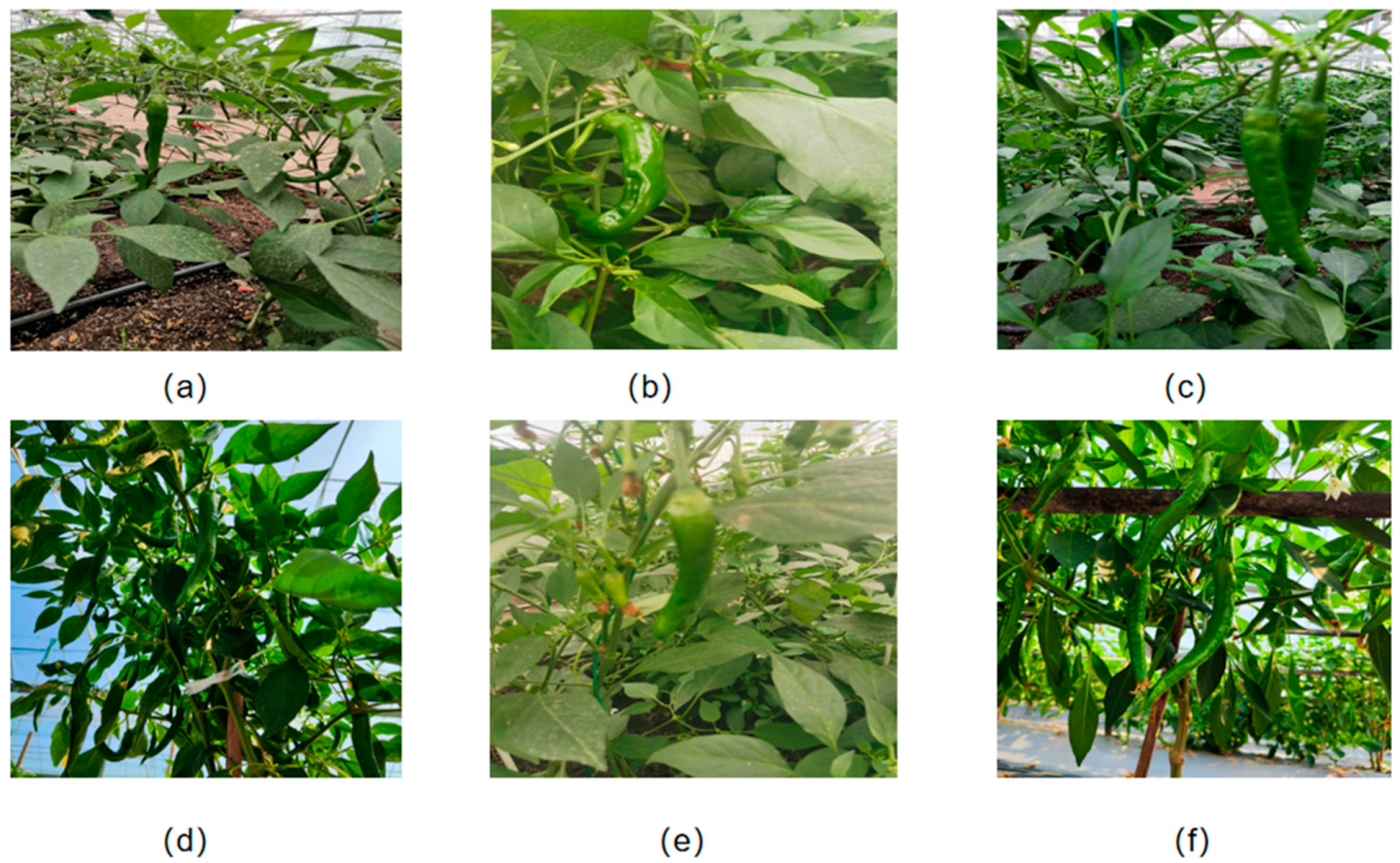
2.1. Data Acquisition

The chili pepper dataset used in this study was obtained from a chili pepper trellis garden in Changsha, Hunan, China. Images were collected under different light conditions at 8:30 a.m., 1:00 p.m., and 5:00 p.m. on 7 May 2022, 2 November 2022, 10 August 2023, and 17 September 2023. The image resolution was 4000 × 4000 pixels. A total of 1456 raw images were collected, of which 762 depicted densely distributed chili peppers and 696 depicted sparsely distributed chili peppers. The densely distributed images included scenarios where chili fruits were occluded by each other, occluded by leaves, and appeared as multiple targets. Details are illustrated in Figure 1. The dataset is publicly available at Kaggle. However, based on our field experience with chili pepper harvesting, automated harvesting faces more complex conditions. While the chili pepper dataset presented in this paper includes most of the weather conditions that may be encountered, it does not cover special conditions such as rainy days, representing a limitation. Additionally, although the dataset contains data on various shading situations and overlapping, it may not accurately identify the exact location of the stalks over time during automatic picking. This limitation will be addressed and optimized in future work.

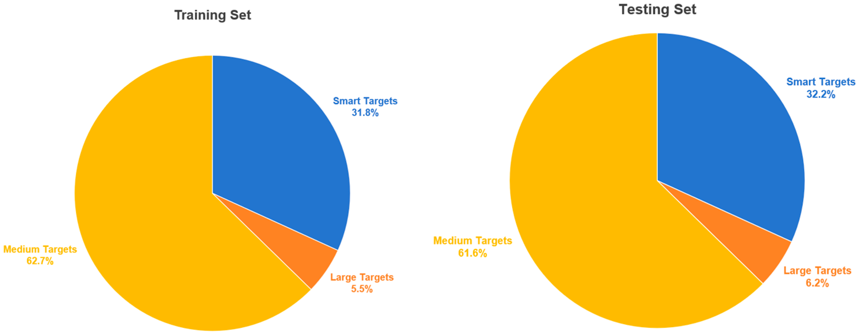
2.2. Data Enhancements

We manually labeled 1456 original images using LabelImg to divide the dataset and test set in the ratio of 8:2. Due to the problem of the original data being too small, we expanded the dataset to 13,176 by adding Gaussian noise (mean = 0, variance = 0.001), random rotation, random brightness change, and random scaling to the dataset, so as to improve the model’s generalization ability and to ensure the model’s practical adaptability. Meanwhile, in order to improve the model’s recognition ability for small target chili peppers, the pre-trained backbone weights on the coco dataset are also used to improve the model’s detection ability. Figure 2 shows the ratio of the number of fruits of different sizes in the training and test sets.

2.3. Experimental Environment

In this paper, the performance of YOLO-chili is investigated for the experimental environment as shown in

Table 1. Experimental Environment.

Configure	Para
CPU	core i5-11400H
GPU	Nvidia GeForce RTX 3050TI
Accelerated environment	CUDA10.1 CUDNN7.5.0
development environment (computer)	Pycharm2020.1.3
operating system	Windows 10 64-bit system
software environment	Anaconda 4.8.4
storage environment	Memory 16.0 GB Mechanical Hard Disk 2 T

.

2.4. HFFN (Hierarchical Feature Fusion Network) Module

In the process of chili pepper detection, it is inevitable that chili pepper targets with different levels of size will appear in the same image, which will seriously interfere with the recognition accuracy of chili peppers. However, the original YOLOv5 feature pyramid is only applicable to the detection of chili pepper targets with a small degree of hierarchical change in chili pepper size, and performs poorly in the detection process where there are chili peppers with large hierarchical changes in an image. In this paper, we introduce adaptive spatial feature fusion (ASFF) in the model to address the above drawbacks and set the convolution kernel in ASFF to a size of 3 × 3 to adapt it to the chili pepper targets in this paper’s dataset. Therefore, YOLO-chili contains a total of three ASFF prediction layers, which are responsible for processing different levels of chili pepper feature information, among which the first layer is the smallest layer of the feature map, with a channel number of 512, which is responsible for processing the feature information of small-scale chili peppers. The second layer is the layer with moderate feature map size and channel number 256, which deals with the feature information of medium-scale chili peppers. The third layer is the layer with the largest feature map, channel number 128, dedicated to processing feature information of large-scale peppers. The YOLO-chili containing three ASFF prediction layers is able to handle chili data with large variations in chili levels in the same map, and thus is fully adapted to the task of chili detection in orchards under complex conditions. The HFFN structure is shown in Figure 3.

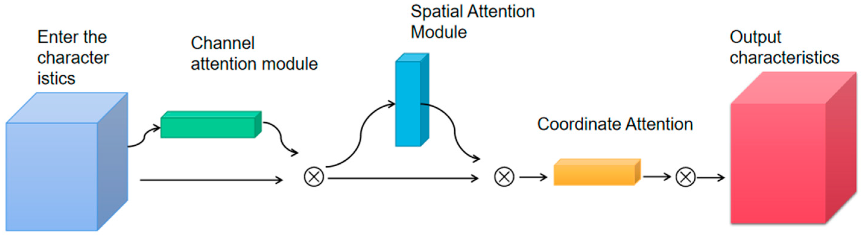
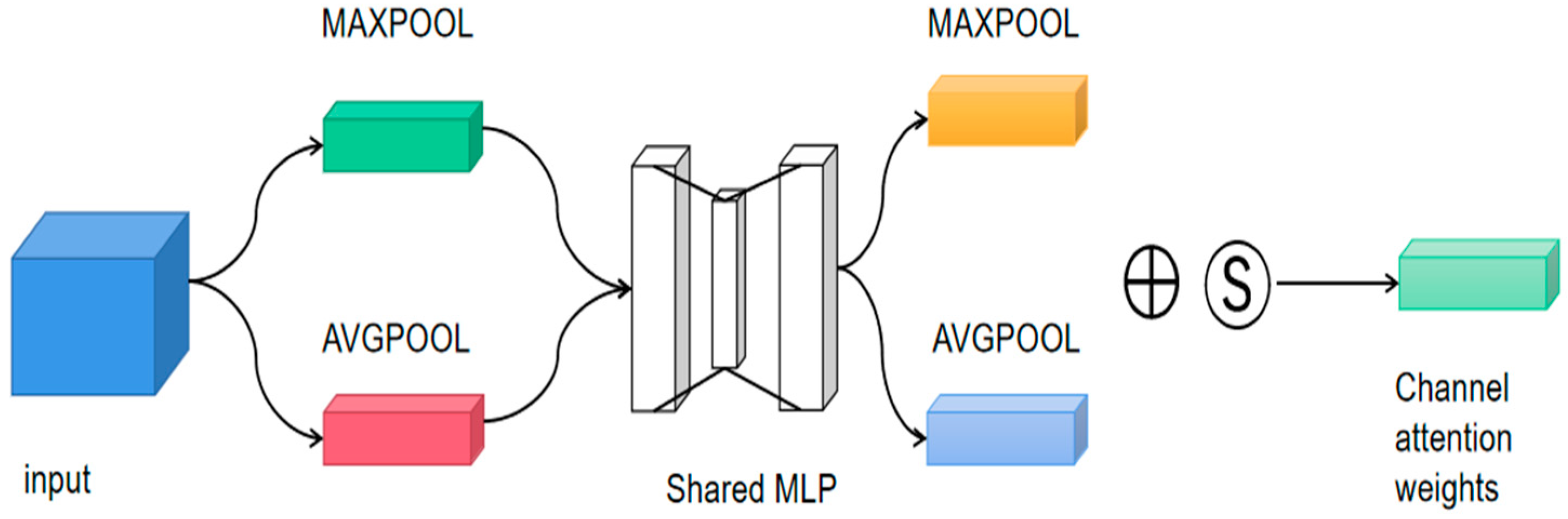
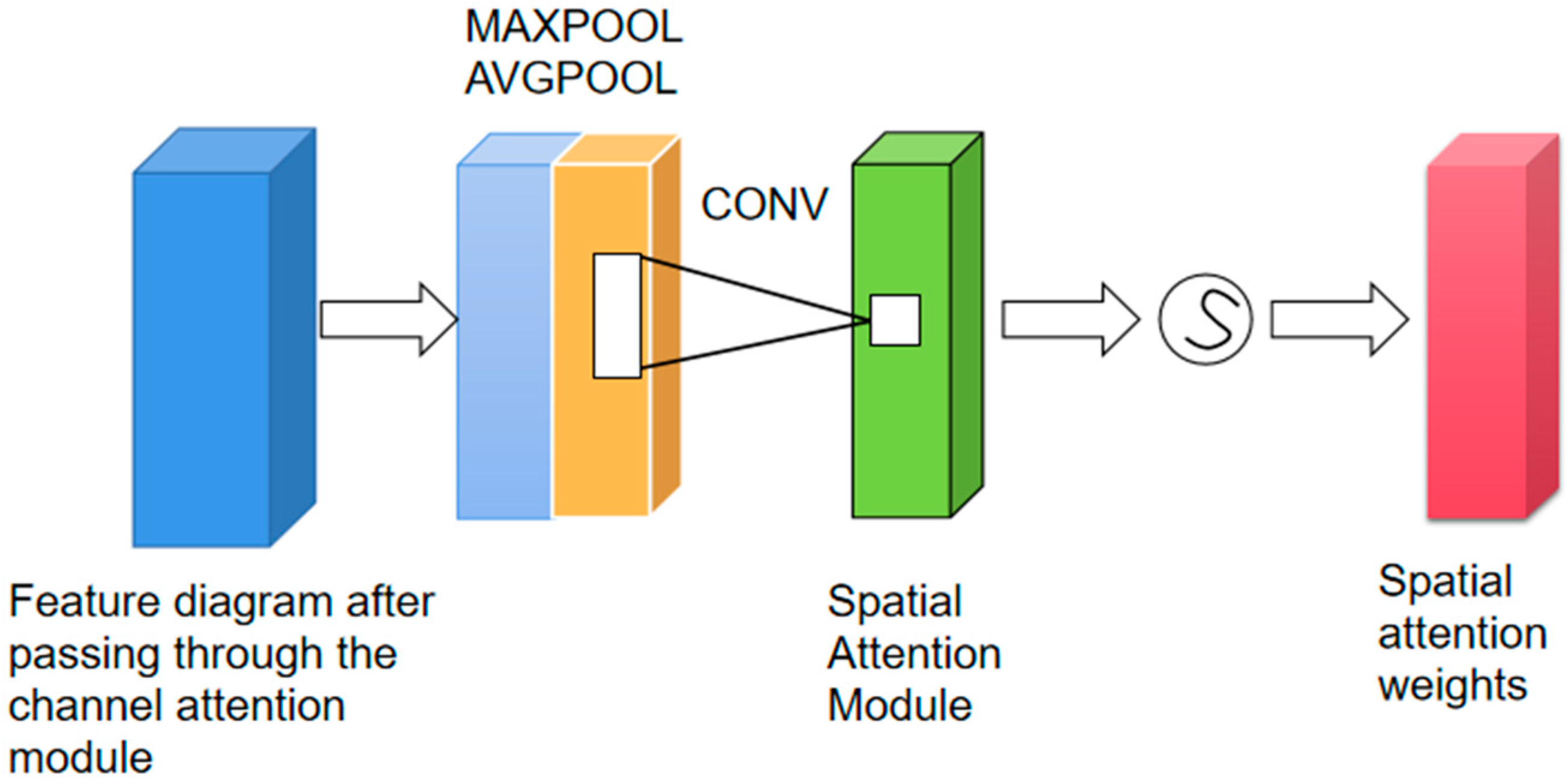
2.5. Three-Channel Attention Mechanism

In HFFN, although YOLO-chili can effectively enhance the detection ability of the model for different layers of targets, it also brings a large amount of environmental noise to the model’s detection, which makes the final detection results receive interference. Therefore, to address the above problems, this paper proposes a three-channel attention mechanism model. Because the three-channel attention mechanism consists of CBAM attention mechanism and CA attention mechanism, it is abbreviated as CBCA module. In this paper, it is added before the feature processing layer of the model and combined with the model, so that the feature information processed by the model is the feature processed by the attention mechanism. In this way, the features processed by the model are enhanced and effective features, and the three-channel attention mechanism module also suppresses the information interference from the complex background in the process, which improves the model performance. The three-channel attention mechanism module, shown in Figure 4, includes a spatial attention module, a channel attention module, and a coordinate attention module, and is a product of the linkage between the three.

The channel attention mechanism is an adaptive spatially selective attention module for dynamically learning and adjusting the importance of different channels (feature maps). It helps the model to effectively interact and transfer information between different channels of the feature map to enhance the model’s representation of the input data. It mainly realizes the deep information representation of pepper targets in images by weighting the convolutional features of the channels. In channel attention, the input feature map F (input) is firstly subjected to global max pooling and global average pooling based on width and height, respectively, to obtain two 1 × 1 × C feature maps. Then, they are fed into a two-layer neural network (MLP) with the number of neurons in the first layer as C/r (r is the reduction rate) and the activation function as Relu, and the number of neurons in the second layer as C. This two-layer neural network is shared. And then, the MLP output features are subjected to element-wise based sum operation and then sigmoid activation operation to generate the final channel attention feature. Finally, the element-wise multiplication operation is performed between the channel attention feature and the input feature map F to generate the input features required by the Spatial attention module. See Figure 5 for details.

The spatial attention mechanism is used to dynamically learn and adjust the importance of different spatial locations. It helps the model to effectively interact and transfer information between different spatial locations of the feature map to enhance the model’s representation of the input data. Specifically, spatial attention is a channel compression technique that performs average pooling and maximum pooling in channel dimensions, respectively. In spatial attention, the feature map output from the Channel attention module is used as the input feature map of this module. Firstly, we perform a channel-based global max pooling and global average pooling to obtain two H × W × 1 feature maps, and then we perform a concat operation (channel splicing) based on the two feature maps. Then we perform a 7 × 7 convolution (7 × 7 is better than 3 × 3) to reduce the dimensionality to 1 channel, i.e., H × W × 1. Then we generate a spatial attention feature, through sigmoid, and finally, we multiply the feature with the input feature of the module to obtain the final generated feature. The detailed structure is shown in Figure 6.

Unlike traditional spatial attention, coordinate attention focuses on the absolute coordinate information of each location in the input feature map, not just the features at the spatial location. Therefore, the coordinate attention module can help the model to obtain the absolute coordinate information of the chili peppers, so as to reduce the interference of environmental factors on the model. Coordinate attention with the help of the idea of the residual module, in the use of C × H × 1 convolution of the features at the same time using a parallel module to process the feature map, and then through the aggregation to obtain two independent feature maps. As shown in Figure 7, the final two independent feature maps are multiplied with the input feature map to obtain the final feature map, thus realizing the absolute expression of coordinate information.

The effective combination of the above modules constitutes a three-channel attention mechanism, which enables the model to effectively capture pepper fruits at different locations when deployed to mobile devices, thus realizing the efficient operation of pepper detection.

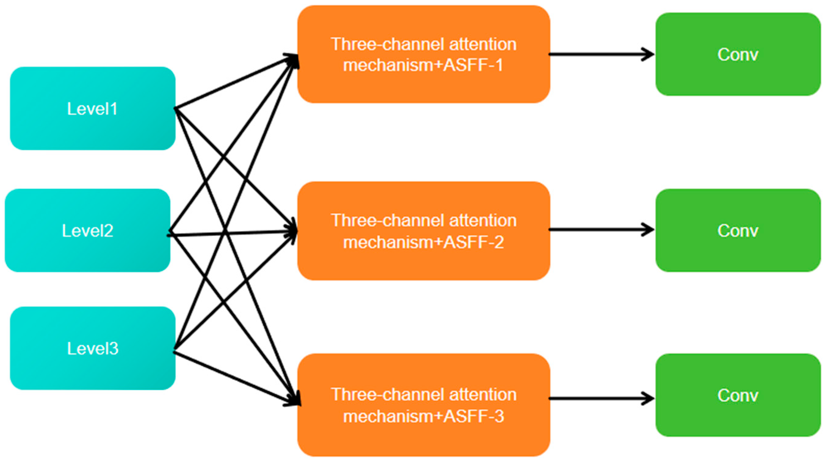
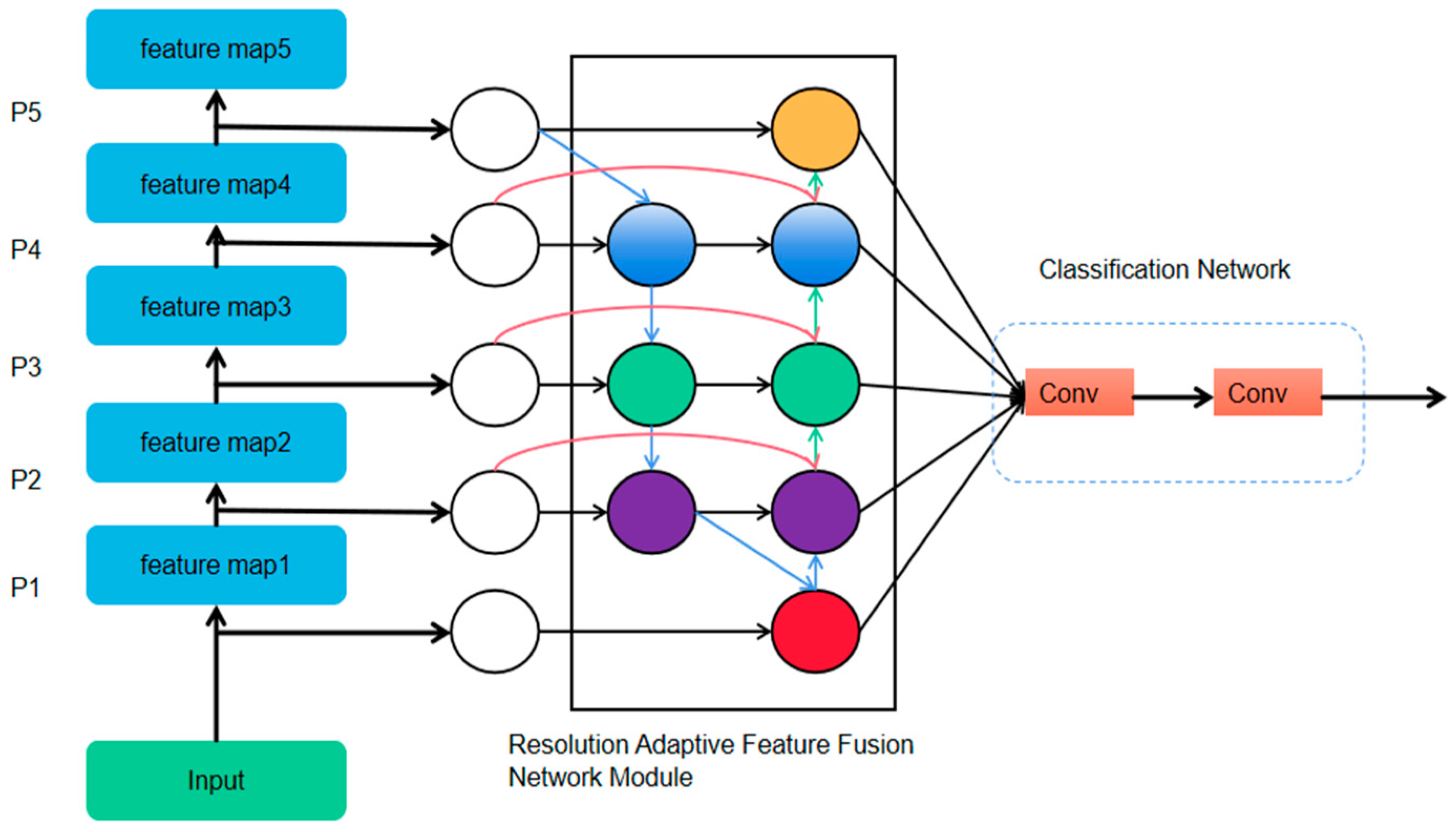
2.6. Resolution Adaptive Feature Fusion Network Module

Because data captured using less than the same equipment will be encountered during the pepper detection process, these data will have different resolutions, while image data captured by the same equipment will also consist of different resolutions. In this paper, we find that the images of chili peppers with different resolutions produce different feature maps when input to the model, and therefore do not contribute differently to the model’s fusion of different features for prediction. To address the above problems, this paper proposes the resolution adaptive fusion module, which aims to aggregate features of different resolutions. Previous models deal with this kind of problem by adjusting the feature maps of different resolutions to the same resolution and then summing them up. The resolution adaptive fusion module, on the other hand, as shown in Figure 8, adds an additional weight to each input and allows the network to learn the importance of each input feature. And the jump connections from input nodes to output nodes are in the same proportion as they are in the same layer, thus fusing more features without adding much computational cost. In addition, a basic network is constructed using each of the networks composed of top-down and bottom-up and repeated several times to achieve higher-level feature fusion.

2.7. YOLO-Chili Network

YOLO-chili is shown in Figure 9, which uses YOLOv5’s backbone network to facilitate porting to different devices. YOLOv5’s backbone network is CSPDarknet53, which consists of CBL, BottleneckCSP/C3, and SPP/SPPF. For ease of deployment, YOLOv5 removes the Focus module. The CBS module consists of a constant combination of Conv+BatchNorm+SiLU used to obtain the depth of the feature map. C3, on the other hand, draws on the residual idea for cross-stage connectivity, which is used to improve the feature transfer efficiency and information utilization. It consists of multiple convolutional layers and residual connections for extracting features from the input image. Compared with CSPDarknet53-tiny in YOLOv4, YOLOv5 has a deeper network structure and stronger feature extraction capability. Meanwhile, for the problem that YOLOv4 cannot handle multi-scale feature maps better, YOLOv5 uses FPN for fusion, which improves the model’s ability to detect targets of different sizes. In terms of prediction, YOLO-chili uses the prediction module of YOLOv5, but uses ASFF-Detect instead of the original detection layer. It also employs the K-Means algorithm to cluster the anchor frames generated from the dataset, the non-great suppression and confidence threshold filtering to select the prediction frames, and Alpha-IoU instead of CIOU. IoU is computed as the ratio of the area of intersection of the target detection frames (which are usually the frames predicted by the model) with the true labeling frames (Ground Truth) and their concatenation area. The value of IoU ranges from 0 to 1. The value ranges from 0 to 1, with larger values indicating a higher degree of overlap between the detected frames and the true labeled frames, and more accurate detection results. α-IoU introduces a parameter α to regulate the calculation of IoU. Specifically, α-IoU is calculated as follows: If the IoU between the detected frame and the real labeled frame is greater than or equal to α, the IoU is directly used as the final evaluation index. If the IoU is less than α, the IoU is multiplied by a factor less than 1 to reduce its influence on the final evaluation index.

3. Results and Discussion

3.1. Parameter Setting

The parameters for the comparison experiments were set as follows: the original size of the image was 640 × 640 pixels, so the input to the model was also adjusted to 640 × 640 × 3. The ratio of the training set to the test set was set to 8:2. The batch size was set to 4, the epoch was set to 100, the initial learning rate was 0.01, the cyclic learning rate was 0.2, and the optimizer used was SGD (stochastic gradient descent), with a weight decay coefficient of 0.0005, and the iou loss coefficient was set to 0.05.

3.2. Evaluation Indicators

In this study, we use precision, F1 score, accuracy and recall as evaluation metrics to assess the effectiveness of different network models in detection tasks targeting chili pepper images, here Equations (1)–(4) are the formulas for F1, accuracy, precision and recall, respectively.

$$F1=\frac{2TP}{2TP+FP+FN}$$

(1)

$$Accuracy=\frac{\mathrm{TP}+\mathrm{TN}}{TP+FP+TN+FN}$$

(2)

$$Precision=\frac{TP}{TP+FP}$$

(3)

$$Recall=\frac{TP}{TP+FN}$$

(4)

where TP is the number of positive samples predicted by the classifier and the true result is positive, i.e., the number of correctly identified positive samples; FP is the number of negative samples predicted by the classifier and the true result is negative, i.e., the number of incorrectly predicted negative samples; FN is the number of positive samples predicted by the classifier and the true result is positive, i.e., the number of underreported positive samples; and TN is the number of negative samples correctly identified. Thus, Accuracy denotes the proportion of correctly classified samples to the total number of samples, Precision denotes the proportion of samples with positive predictions that are actually positive samples, Recall denotes the proportion of the number of actual positive samples in samples with positive measurements to the proportion of positive samples in the full sample, and F1 is a weighted average of Precision and Recall.

3.3. YOLO-Chili Ablation Test Performance Comparison

In this paper, ablation experiments were conducted on the test set using YOLO-chili to verify the feasibility of the model optimization strategy based on YOLO-chili. As shown in

Table 2. Ablation Test Performance Comparison.

YOLO-Chili	HFFN	Three-Channel Attention Mechanism	Resolution Adaptive Feature Fusion Network Module	AP (Average Precision) (%)	Precision (%)	Recall (%)
✓				83.24	91.33	81.77
✓		✓		91.39	92.74	91.65
✓	✓			82.32	87.93	81.62
✓			✓	85.54	93.54	82.15
✓	✓		✓	92.24	93.42	91.19
✓	✓	✓		91.27	93.20	91.62
✓	✓	✓	✓	94.11	94.42	92.25

✓ Represents the Use of Such Modules.

, it can be seen that after adding HFFN, three-channel attention mechanism and Resolution Adaptive Feature Fusion Network Module, all the indexes are improved. However, by adding only HFFN, all the performances are decreased, which is due to the problem of positive and negative sample confusion that occurs when YOLO-chili performs different levels of feature fusion, and at the same time, the features of the level fusion have a great deal of background noise, which seriously interferes with the model’s prediction; therefore, by adding the three-channel attentional mechanism prior to the HFFN, the performance of the model is significantly improved due to the three-channel attention mechanism suppressing the interference of background noise and highlighting the fruit features. However, due to the addition of different modules, the computational complexity and memory consumption of the network increased accordingly.

3.4. Comparison of the Performance of Different Object Detection Models

The comparison between the YOLO-chili model and the currently mainstream object detection models, including Faster-RCNN, SSD, YOLOv7, YOLOv7-tiny, and YOLOv5, is presented in

Table 3. Detection Results of Different Target Detection Algorithms.

Models	Parameters/M	FLOPs/G	Model Size/MB	AP (%)	Precision (%)	Recall (%)	Test Time/ms
YOLOv5	7.24	16.6	14.1	85.53	91.33	81.77	47.7
YOLOv7	37.49	123.5	74.5	92.39	94.24	91.65	97.2
YOLOv7-tiny	6.51	14.2	12.1	89.32	93.93	87.62	46.8
SSD	26.29	62.8	93.3	91.24	93.42	73.19	65.5
Faster-RCNN	137.10	370.2	111.5	83.63	67.84	81.62	126.3
YOLO-chili	11.4	21.2	18.7	94.11	94.42	92.25	55.4

. All models use the default configuration after downloading, except for the YOLO-chili model presented in this paper, which is detailed in Section 3.1. The average precision mean of the YOLO-chili model is, respectively, 10.48, 2.87, 0.18, 0.49, and 3.09 percentage points higher than the other five models. Among them, the single-stage detection network model SSD has the lowest recognition accuracy, and the two-stage detection model Faster-RCNN has the largest number of parameters, thus leading to slower inference speed. The average precision mean and inference speed of YOLOv7 are improved compared to Faster-RCNN and SSD, but it still cannot meet the requirement of real-time detection for pepper fruits. Although the precision of the YOLO-chili model is only slightly higher than that of YOLOv7-tiny, the parameter count is much higher than that of YOLOv7-tiny. While it can meet the requirement for real-time detection of pepper fruits, further optimization is still necessary. In particular, the test time in Table 3 is the time it takes for the model to detect an image.

As can be seen in Figure 10, the YOLO-chili model has the fastest fitting speed, while the curve change of Faster-RCNN is obviously unstable, which is due to the efficiency of the YOLO series model as a one-stage model itself. The YOLO-chili, on the other hand, is due to the possession of efficient computational power and the use of transfer learning to acquire sufficient prior knowledge. At the same time, traditional SSDs may not be able to adapt to the complex and changing environment of the chili dataset and the complexity of the model, thus making it the slowest to train. For the complex environment of the chili pepper dataset YOLOv7-tiny does not seem to outperform YOLO7, but both are using a migration learning approach and therefore both are slower to fit. It can be inferred from the results that the model performance of both YOLOv7 and YOLO-chili is suitable for the real-time detection of chili peppers.

3.5. Reducing Model Size Using Quantitative Pruning

The ultimate goal of this paper is to deploy the real-time detection model to different hardware devices. Therefore, lightweighting is a necessary optimization step, and we use the quantitative pruning algorithm to prune the model to reduce the number of model parameters and improve the speed of the model by pruning the channels that account for a lower percentage of importance in the model. First, we use YOLO-chili to train the model in the fitted state, and then perform quantitative pruning on the trained model. At the same time, the sparsity of the lower weight layer is trimmed from 0.5 to 0.9 and then the model is quantized and compressed. After that, this paper retrains the YOLO-chili model until it converges. This method can effectively reduce the model parameters, model computational complexity, and the size of the weight file while preserving the accuracy of the model. The results are shown in

Table 4. Quantitative Pruning Results.

Models	M-Params	AP	Recall	Precision	FPS
YOLO-chili	18.7	94.11	92.25	94.42	94
pruned_quantized_model	9.64	93.66	97	97	87

. The original model parameters are 18.7 M, and after quantized training of the model weight file, the pruned model parameters are 9.64 M, and the model accuracy reaches 93.66%, which is only 0.45% decrease in accuracy, while the model volume is reduced by half, and the FPS is only 65, which makes YOLO-chili fully adaptable to a variety of different mobile devices to accomplish the real-time detection tasks. Although the effect of FPS is reduced, this is acceptable compared to the improvement in detection performance.

The detection results of YOLO-chili are presented in Figure 11. These results demonstrate that YOLO-chili can effectively identify the location of chili peppers in complex scenarios, including multilayered targets, cloudy skies, and occlusion, thereby validating the algorithm’s effectiveness. However, as shown in the bottom left corner of the second image in Figure 11, the model fails to detect a chili pepper because only a quarter of the pepper is visible, highlighting a limitation in detecting partially exposed fruits. Our observations indicate that different lighting conditions have minimal impact on the automatic detection of pepper fruits. Instead, factors such as occlusion by other fruits and debris, like leaves, and the color similarity between the leaves and the fruits significantly affect the detection performance.

4. Conclusions

In this paper, we propose a YOLOv5-based pepper target detection algorithm, YOLO-chili. The initial YOLOv5 model performs inadequately in recognizing small target peppers, dimly lit peppers, and clusters of peppers. Therefore, we introduce a Hierarchical Feature Network (HFNN) to enhance detection across different layers of target peppers. Additionally, we incorporated a long-range information extraction module into the CBAM Attention Module and developed a three-channel attention mechanism network. This network aims to mitigate the impact of complex backgrounds on chili pepper detection, thereby improving overall detection performance. Furthermore, we replaced the original Intersection over Union (IOU) function with the Alpha-IOU loss function and utilized a resolution-adaptive feature fusion network module to merge features at various resolutions. Quantized pruning was employed to manage model size, ensuring the model’s lightweight nature. Experimental results demonstrate that YOLO-chili is fully adaptable to the task of pepper picking in real-world scenarios and achieves real-time detection speeds suitable for practical applications. Future research will focus on utilizing YOLO-chili for real-time detection of various types of peppers to advance the intelligence and modernization of the pepper-picking process. Although we addressed the detection of chili peppers in complex environments, the detection of chili stalk separation remains unresolved, presenting a significant challenge in automated chili pepper harvesting. Additionally, detecting peppers at different ripening stages is essential and will be a focus of future research endeavors.

References

1. Fu, L.; Duan, J.; Zou, X.; Lin, J.; Zhao, L.; Li, J.; Yang, Z. Fast and accurate detection of banana fruits in complex background orchards. IEEE Access 2020, 8, 196835–196846. [Google Scholar] [CrossRef]
2. Mathew, M.P.; Mahesh, T.Y. Leaf-based disease detection in bell pepper plant using YOLOv5. Signal Image Video Process. 2022, 16, 841–847. [Google Scholar] [CrossRef]
3. Tian, Y.; Yang, G.; Wang, Z.; Wang, H.; Li, E.; Liang, Z. Apple detection during different growth stages in orchards using the improved YOLO-V3 model. Comput. Electron. Agric. 2019, 157, 417–426. [Google Scholar] [CrossRef]
4. Liu, T.H.; Nie, X.N.; Wu, J.M.; Zhang, D.; Liu, W.; Cheng, Y.F.; Qi, L. Pineapple (Ananas comosus) fruit detection and localization in natural environment based on binocular stereo vision and improved YOLOv3 model. Precis. Agric. 2023, 24, 139–160. [Google Scholar] [CrossRef]
5. Gai, R.; Chen, N.; Yuan, H. A detection algorithm for cherry fruits based on the improved YOLO-v4 model. Neural Comput. Appl. 2023, 35, 13895–13906. [Google Scholar] [CrossRef]
6. Jiang, M.; Song, L.; Wang, Y.; Li, Z.; Song, H. Fusion of the YOLOv4 network model and visual attention mechanism to detect low-quality young apples in a complex environment. Precis. Agric. 2022, 23, 559–577. [Google Scholar] [CrossRef]
7. Yang, G.; Wang, J.; Nie, Z.; Yang, H.; Yu, S. A lightweight YOLOv8 tomato detection algorithm combining feature enhancement and attention. Agronomy 2023, 13, 1824. [Google Scholar] [CrossRef]
8. Tian, Y.; Wang, S.; Li, E.; Yang, G.; Liang, Z.; Tan, M. MD-YOLO: Multi-scale Dense YOLO for small target pest detection. Comput. Electron. Agric. 2023, 213, 108233. [Google Scholar] [CrossRef]
9. Lin, Y.; Huang, Z.; Liang, Y.; Liu, Y.; Jiang, W. AG-YOLO: A Rapid Citrus Fruit Detection Algorithm with Global Context Fusion. Agriculture 2024, 14, 114. [Google Scholar] [CrossRef]
10. Yang, S.; Xing, Z.; Wang, H.; Dong, X.; Gao, X.; Liu, Z.; Zhang, X.; Li, S.; Zhao, Y. Maize-YOLO: A new high-precision and real-time method for maize pest detection. Insects 2023, 14, 278. [Google Scholar] [CrossRef]
11. Zhao, Y.; Yang, Y.; Xu, X.; Sun, C. Precision detection of crop diseases based on improved YOLOv5 model. Front. Plant Sci. 2023, 13, 1066835. [Google Scholar] [CrossRef] [PubMed]
12. Karthikeyan, M.; Subashini, T.S.; Srinivasan, R.; Santhanakrishnan, C.; Ahilan, A. YOLOAPPLE: Augment YOLOv3 deep learning algorithm for apple fruit quality detection. Signal Image Video Process. 2024, 18, 119–128. [Google Scholar] [CrossRef]
13. Tang, R.; Lei, Y.; Luo, B.; Zhang, J.; Mu, J. YOLOv7-Plum: Advancing plum fruit detection in natural environments with deep learning. Plants 2023, 12, 2883. [Google Scholar] [CrossRef] [PubMed]
14. Parico, A.I.B.; Ahamed, T. Real time pear fruit detection and counting using YOLOv4 models and deep SORT. Sensors 2021, 21, 4803. [Google Scholar] [CrossRef]
15. Lawal, O.M.; Huamin, Z.; Fan, Z. Ablation studies on YOLOFruit detection algorithm for fruit harvesting robot using deep learning. In IOP Conference Series: Earth and Environmental Science; IOP Publishing: Bristol, UK, 2021; Volume 922, p. 012001. [Google Scholar]
16. Li, T.; Sun, M.; Ding, X.; Li, Y.; Zhang, G.; Shi, G.; Li, W. Tomato recognition method at the ripening stage based on YOLO v4 and HSV. Trans. Chin. Soc. Agric. Eng. (Trans. CSAE) 2021, 37, 183–190. [Google Scholar]
17. Guo, J.; Xiao, X.; Miao, J.; Tian, B.; Zhao, J.; Lan, Y. Design and Experiment of a Visual Detection System for Zanthoxylum-Harvesting Robot Based on Improved YOLOv5 Model. Agriculture 2023, 13, 821. [Google Scholar] [CrossRef]
18. Yang, J.; Qian, Z.; Zhang, Y.; Qin, Y.; Miao, H. Real-time recognition of tomatoes in complex environments based on improved YOLOv4-tiny. Trans. Chin. Soc. Agric. Eng. (Trans. CSAE) 2022, 38, 215–221. [Google Scholar]
19. Wang, L.; Qin, M.; Lei, J.; Wang, X.; Tan, K. Blueberry maturity recognition method based on improved YOLOv4-Tiny. Trans. Chin. Soc. Agric. Eng. (Trans. CSAE) 2021, 37, 170–178. [Google Scholar]
20. Sun, F.; Wang, Y.; Lan, P.; Zhang, X.; Chen, X.; Wang, Z. Identification of Apple Fruit Diseases Using Improved YOLOv5s and Transfer Learning. Trans. Chin. Soc. Agric. Eng. 2022, 38, 171–179. [Google Scholar]
21. Ren, R.; Zhang, S.; Sun, H.; Liu, J.; Cheng, J.; Li, Y.; Wang, Q. Research on Pepper External Quality Detection Based on Transfer Learning Integrated with Convolutional Neural Network. Sensors 2021, 21, 5305. [Google Scholar] [CrossRef] [PubMed]
22. Zhou, J.; Hu, W.; Zou, A.; Liu, H.; Zhang, Q.; Wu, X.; Zheng, H. Lightweight Detection Algorithm of Kiwifruit Based on Improved YOLOX-s. Agriculture 2022, 12, 993. [Google Scholar] [CrossRef]
23. Zhang, C.; Kang, F.; Wang, Y. An Improved Apple Object Detection Method Based on Lightweight YOLOv4 in Complex Backgrounds. Remote Sens. 2022, 14, 4150. [Google Scholar] [CrossRef]
24. Wang, D.; He, D. Channel Pruned YOLO V5s-Based Deep Learning Approach for Rapid and Accurate Apple Fruitlet Detection Before Fruit Thinning. Biosyst. Eng. 2021, 210, 271–281. [Google Scholar] [CrossRef]
25. Gou, J.; Yu, B.; Maybank, S.J.; Tao, D. Knowledge Distillation: A Survey. Int. J. Comput. Vis. 2021, 129, 1789–1819. [Google Scholar] [CrossRef]
26. Wang, F.; Jiang, J.; Chen, Y.; Li, H.; Zhang, S.; Luo, Q.; Liu, X. Rapid Detection of Yunnan Xiaomila Based on Lightweight YOLOv7 Algorithm. Front. Plant Sci. 2023, 14, 1200144. [Google Scholar] [CrossRef]
27. Fu, L.; Yang, Z.; Wu, F.; Liu, S.; Zhao, C.; Zhao, Z.; Xiong, J.; Guo, Y. YOLO-Banana: A Lightweight Neural Network for Rapid Detection of Banana Bunches and Stalks in the Natural Environment. Agronomy 2022, 12, 391. [Google Scholar] [CrossRef]
28. Fang, W.; Guan, F.; Yu, H.; Wang, Y.; Li, J.; Zhang, X. Identification of Wormholes in Soybean Leaves Based on Multi-Feature Structure and Attention Mechanism. J. Plant Dis. Prot. 2023, 130, 401–412. [Google Scholar] [CrossRef]
29. Abade, A.; Ferreira, P.A.; de Barros Vidal, F. Plant diseases recognition on images using convolutional neural networks: A systematic review. Comput. Electron. Agric. 2021, 185, 106125. [Google Scholar] [CrossRef]
30. Zeng, W.; Li, M. Crop Leaf Disease Recognition Based on Self-Attention Convolutional Neural Network. Comput. Electron. Agric. 2020, 172, 105341. [Google Scholar]
31. Gu, J.; Wang, Z.; Kuen, J.; Ma, L.; Shah, R.; He, K.; Zhao, Y.; Da Xu, X.; Liu, T.; Wang, G. Recent Advances in Convolutional Neural Networks. Pattern Recognit. 2018, 77, 354–377. [Google Scholar] [CrossRef]
32. Yu, L.; Xiong, J.; Fang, X.; Yang, Z.; Chen, Y.; Lin, X.; Chen, S. A litchi fruit recognition method in a natural environment using RGB-D images. Biosyst. Eng. 2021, 204, 50–63. [Google Scholar] [CrossRef]
Figure 1. Photographs of chili peppers in different light with different shooting angles. (ac) show peppers photographed in cloudy weather, and (df) show peppers photographed in sunny weather. The shooting angles of chili peppers were categorized into top, top and flat views.
Applsci 14 05524 g001
Figure 2. Distribution of chili peppers at different scales in the chili pepper dataset.
Applsci 14 05524 g002
Figure 3. HFFN Structure.
Applsci 14 05524 g003
Figure 4. Diagram of the Three-Channel Attention Mechanism Structure.
Applsci 14 05524 g004
Figure 5. Channel Attention Module.
Applsci 14 05524 g005
Figure 6. Spatial Attention Module.
Applsci 14 05524 g006
Figure 7. Coordinate Attention Module.
Applsci 14 05524 g007
Figure 8. Resolution Adaptive Feature Fusion Network Module.
Applsci 14 05524 g008
Figure 9. YOLO-chili Structure.
Applsci 14 05524 g009
Figure 10. Comparison of Learning Convergence.
Applsci 14 05524 g010
Figure 11. YOLO-chili Test Results.
Applsci 14 05524 g011