Automated Trucks’ Impact on Pavement Fatigue Damage

Abstract

The automated truck’s steering system can potentially control its lateral movement (i.e., wander mode) within the lane. The controlled wander mode of automated trucks could affect the transverse loading distribution of the wheels and consequently influence pavement fatigue damage in the long term. This study examines the effects of potential wander modes on pavement fatigue damage, considering the effects of lane width, market penetration rate, flexible pavement layers’ thickness, and stiffness of the materials. This study uses a finite element model to calculate the flexible pavement response. The mechanistic–empirical method is used to compute the total fatigue damage index for a specific design period, incorporating the wander mode effect. Comparing the fatigue damage indices indicates that automated trucks could either reduce the damage index value from −1.41% to −7.05% (i.e., mitigator scenario) or increase it from +11.6% to +278.57% (i.e., aggravator scenario), depending on their deployment scenarios. Moreover, the findings show that using a uniform-wander mode instead of a zero-wander mode or increasing the thickness and stiffness of the pavement layers could effectively reduce the adverse effect of automated trucks on fatigue damage and reduce the damage indices from −0.06% to −42.95%. However, their impact is considerably influenced by market penetration rate and lane width.

1. Introduction

Pavement structure analysis and design are crucial in ensuring that pavement can effectively accommodate truck traffic. In recent years, the implementation of automated driving technology into trucks has garnered significant attention due to its potential to provide a range of benefits to freight transportation, including reduced operational costs, improved fuel efficiency, and enhanced road safety [1,2,3,4,5,6,7]. However, it is essential to consider the potential differences between automated trucks (ATs) and human-driven trucks (HDTs), which could impact pavement performance differently [1,2,8,9,10,11,12,13,14,15,16,17,18,19,20,21].

Among the potential differences between ATs and HDTs, one of the critical factors to consider is the programmable capability of ATs’ lateral wandering pattern. This capability allows ATs to follow a pre-programmed wander mode either individually within a lane or in a synchronised manner (i.e., truck platooning). In other words, we can envision two primary approaches for implementing the proposed wander modes for ATs: individual wandering and cooperative wandering. In the individual wandering approach, each AT swings within its lane, adhering to the proposed wander mode. This means that the lateral position of each vehicle would vary over time, similar to the behaviour observed in HDTs. Each vehicle’s lateral movement would be independent, creating a dynamic pattern within the lane. In contrast, the cooperative wandering approach involves synchronising the lateral positions of all ATs within a platoon. Here, the lateral position of each vehicle would be fixed but slightly offset from one another. This synchronisation means that the number of ATs at each transverse point would collectively form the proposed wander mode. However, achieving the cooperative wandering approach realistically hinges on the presence of connected vehicle technology, a sufficient number of ATs, and supporting infrastructure. This interconnectivity allows for precise synchronisation and coordination among the vehicles, ensuring their lateral positions can be adjusted in real-time to maintain the desired wander pattern. Without such technology, the coordination required for the cooperative wandering approach would be exceedingly challenging.

Researchers have proposed various potential wander modes, including zero, uniform-time, uniform-frequency, two-section-uniform, normal, double peak Gaussian, and Laplace for ATs [8,15,16,17,22,23,24]. These studies have indicated significant differences in the induced fatigue and rutting damage between different ATs’ wander modes. However, it is essential to acknowledge that the impact of the wander mode of ATs on pavement performance is also influenced by additional factors such as lane distribution management, market penetration, lane width, and structural characteristics of flexible pavements, as discussed in the subsequent sections [9,15,16,18,21,25].

As ATs gradually become more prevalent on roads, mixed traffic conditions involving different market penetration rates may arise. Alternatively, an exclusive lane may be designated for ATs. Combining the programmed wander mode of ATs with the normal lateral wandering of HDTs (i.e., integrated scenarios) or employing 100% ATs in a separated lane (i.e., segregated scenarios) can lead to various transverse wheel load distribution scenarios, which can affect pavement rutting and fatigue life. In this context, previous studies have demonstrated that as the market penetration rate of ATs increases, the impact of the wander mode of ATs on pavement fatigue performance becomes more pronounced [16].

Due to the ATs’ controlled wandering system, researchers have indicated that ATs have the potential to use narrower lanes, which could save construction and maintenance costs [26,27,28,29]. However, using narrower lanes could considerably influence pavement performance in various wander modes and penetration rates, as Yeganeh et al. [9] demonstrated. This study showed that in the case of implementing a zero-wander mode for ATs, the variations in total rutting depth across different lane widths are more pronounced at lower penetration rates as opposed to higher penetration rates, which is contrary to what is observed when using a uniform-wander mode. Nevertheless, to the best of our knowledge, the lane width effect on pavement fatigue damage for different ATs’ wander modes has not been investigated in the literature.

In addition, the characteristics of the flexible pavement structure (e.g., layers’ thickness and stiffness) could contribute to the structural response of pavement under various wander modes and consequently affect pavement fatigue performance. In this regard, Georgouli and Plati [8] showed that using normal, uniform, and Laplace distributions instead of zero distribution could result in a reduction in fatigue cracking (FC) of hot mix asphalt (HMA). They indicated that the FC reduction varies with the thickness and stiffness of the material. Specifically, their findings demonstrated that for every 2-centimetre increase in HMA thickness, the FC reduction decreases by 5% to 6%. In contrast, an increase of 1000 MPa in HMA stiffness has a minor effect, with the decrease in FC reduction ranging from 1% to 2.2% [8]. They employed the methodology proposed in the mechanistic–empirical pavement design guide (MEPDG), developed by McCullah and Gray [30], to account for the wheel wander effect. However, as Coca et al. [31] pointed out, this approach may produce inaccurate results due to its discretisation of the wheel frequency distribution into only five segments. Furthermore, the effects of market penetration rate and lane width were not considered in the mentioned study.

Despite the studies discussed above, there is still a limited understanding of ATs’ impact on pavement fatigue performance. Thus, this research aims to enhance the current knowledge by considering the effects of lane distribution scenarios, ATs’ market penetration rate, lane width, pavement layers’ thickness, and material stiffness concerning ATs’ wander mode effect on pavement fatigue damage.

Research Problem Statement and Research Objectives

As discussed above, significant technological advances in ATs offer potential benefits such as reduced energy consumption, pollution, driver stress, and congestion costs, along with increased highway capacity, safety, green mobility, efficient freight transportation, and the feasibility of alternative fuel vehicles [32,33,34]. However, a crucial gap exists in understanding the differential impacts of ATs and HDTs on pavement structures. This gap arises from the lack of comprehensive studies comparing the long-term effects of these vehicle types on pavement performance, which is essential for designing pavements that can effectively support both types of vehicles.

ATs can follow pre-programmed wandering patterns, ranging from no-wander to normal and uniform-wander modes. While some research has been initiated on how these patterns affect pavement damage, significant gaps remain in understanding how these wandering algorithms influence pavement fatigue performance under various deployment scenarios. As ATs increasingly populate roads, they will coexist with HDTs, leading to mixed traffic conditions. The current understanding of integrating ATs with different market penetration rates and wandering patterns and their impacts on pavement life in mixed-traffic scenarios is limited. Moreover, controlled wandering systems of ATs allow for the possibility of narrower lanes, potentially resulting in significant construction and maintenance savings. However, the impact of lane width on pavement performance, particularly under different AT penetration rates and wander modes, is not well-documented. Research must determine how these factors interact to influence fatigue damage. A comprehensive understanding of how various pavement structural characteristics, such as thickness and stiffness, respond to these wandering patterns and market penetrations is also lacking. Detailed research is needed to evaluate how different material properties and pavement constructions withstand the mechanical stresses imposed by ATs, ensuring the long-term viability of pavement performance.

In summary, the transition towards increased usage of ATs introduces unique challenges to pavement performance analysis. The main goal of this study is to investigate the fatigue performance of flexible pavements under the influence of ATs and HDTs, considering various wandering patterns, market penetration rates, and pavement structural characteristics as described in the following objectives:

• Assess the comparative impact of ATs relative to HDTs: Evaluate the differential effects of ATs and HDTs on pavement fatigue performance.
• Assess the wandering effect: Explore how different lateral movement patterns (wander modes) of ATs impact pavement fatigue.
• Assess the lane width effect: Examine how varying lane widths influence the fatigue performance of pavements under AT traffic.
• Assess the market penetration effect: Determine the impact of different market penetration rates of ATs on pavement fatigue.
• Assess the layers’ material and thickness effect: Investigate how different pavement layer thicknesses and material properties affect the fatigue performance under AT-induced stresses.

2. Materials and Methods

This study considered several typical three-layer flexible pavement structures (i.e., surface, base, and subgrade layer) that incorporated variable thicknesses and stiffnesses (i.e., elastic modulus) for the base and surface layers. We calculated critical horizontal strain responses under a dual tyre load in the transversal points and determined fatigue damage indices (DI) for each pavement structure. Afterwards, we simulated the zero and uniform wheel wanders for each lane width and market penetration rate scenario and incorporated them into the total fatigue damage index calculation. The following sections describe the flexible pavement cross-sections, fatigue damage computation, and wheel wander incorporation.

2.1. Flexible Pavement Cross-Section Combinations

This study considered a typical flexible pavement structure consisting of an HMA layer and a base layer placed on a subgrade layer. The thickness of the HMA and base layers could significantly impact the pavement fatigue performance [19,32]. Therefore, to account for this, the present study proposed different thicknesses for the HMA layer (i.e., 10 cm, 15 cm, and 20 cm) and the base layer (i.e., 20 cm and 40 cm). Another significant factor affecting the pavement strain response is the mechanical behaviour of the layers’ material. To account for this factor, the study assumed three different reasonable stiffness values for the HMA layer (i.e., 3100 MPa, 6200 MPa, 9300 MPa) with a Poisson’s ratio of 0.3 and two values for the base layer (i.e., 300 MPa and 600 MPa) with a Poisson’s ratio of 0.35. An infinite layer with a stiffness of 100 MPa and a Poisson’s ratio of 0.4 was considered for the subgrade layer. Hence, this study examined 36 combinations of flexible pavement cross-sections varying in thickness and stiffness of the HMA and base layers (see

Table 1. Flexible pavement cross-section combinations.

Layer	Thickness (cm)	Stiffness (MPa)	Poisson’s Ratio
HMA Layer	10, 15, 20	3100, 6200, 9300	0.3
Base Layer	20, 40	300, 600	0.35
Subgrade Layer	Assumed to be infinite thickness	100	0.4

). It is essential to acknowledge that assuming the flexible pavement layers, characterised solely by Young’s modulus and Poisson’s ratio, simplifies the material behaviour. While this assumption provides a practical and commonly used approach, it is important to recognise that real-world materials may exhibit more complex mechanical responses. Future studies could explore more sophisticated material models to capture a broader range of material behaviours, and this consideration will be valuable for refining the accuracy of our analyses.

2.2. Fatigue Damage Computation

The initial stage of this study involved the computation of critical strain values that resulted from a dual tyre loading on each pavement structure composition mentioned above. Considering the traffic data used by Zhou et al. [17], the study assumes that the pavement structure would carry 30 million standard equivalent 80 kN single axle loads over a 20-year design period. This translates to each model dual tyre receiving a load of 40 kN, with each tyre of the dual tyre set receiving 20 kN. Specifically, the contact area of the dual tyre comprises two rectangles, each measuring 0.1981 m in length and 0.1930 m in width. The tyre pressure exerted on the pavement, consistently assumed at 523.31 kPa across the contact area, aligns with Hua’s study, which standardises the pressure distribution over the tyre–pavement interface. Given that each dual tyre set supports 40 kN, an axle, which has two dual tyre sets, supports a total load of 80 kN. This load value represents the standard equivalent single axle load of 80 kN used in pavement design and fatigue analysis. The centre-to-centre distance of the rectangular areas is assumed to be 0.335 m. Since this study focuses on the bottom-up (BU) fatigue damage (i.e., fatigue cracking that begins at the bottom of the asphalt layer and propagates to the surface), the horizontal strain values at the bottom of the HMA layer are determined via the finite element method (FEM) using the commercial software ABAQUS 2020 [33]. The maximum horizontal tensile strains at the bottom of the HMA layer are the critical strain values for BU fatigue damage.

This study used the method proposed by Coca et al. [31] to incorporate wheel wander in fatigue damage computation. For this purpose, we determined the horizontal strains at the bottom of the surface layer in the centre of the loading area and 89 lateral points to the right and left of the centre point by the interval value of 30 mm.

In the next step, the calculated strain values are considered to calculate the DI value in the assumed lateral points at the bottom of the $HMA$ layer after one wheel pass. To this end, the present study used Miner’s rule concept proposed in the MEPDG [30], as shown in Equation (1):

$$DI=\sum {\left(\Delta DI\right)}_{j,m,l,p,T}=\sum {\left(\frac{n}{N_{f-HMA}}\right)}_{j,m,l,p,T}$$

(1)

where $n$ is the actual number of axle-load applications within a specific period, $j$ is the axle-load interval, as obtained from weight in motion (WIM) data, $m$ is the axle-load type (e.g., single, tandem, tridem, quad, or any other particular configuration), $l$ is the truck type, $p$ is the month, $T$ is the median temperature for the five temperature intervals or quintiles used to subdivide each month, and $N_{f-HMA}$ is the allowable number of axle load repetitions. The allowable number of axle load repetitions ($N_{f-HMA})$ can be calculated with Equation (2) [30]:

$$N_{f-HMA}=k_{f1}\left(C\right)(C_H){\beta }_{f1}{\left({\epsilon }_t\right)}^{k_{f2}{\beta }_{f2}}{\left(E_{HMA}\right)}^{k_{f3}{\beta }_{f3}}$$

(2)

where ${\epsilon }_t$ is the tensile strain at critical locations in inches, $E_{HMA}$ is Young’s modulus of the $HMA$ in psi, $k_{f1},k_{f2},k_{f3}$ are the global field calibration parameters ($k_{f1}=0.007566$, $k_{f2}=-3.9492$, and $k_{f3}=-1.281$), ${\beta }_{f1},{\beta }_{f2},{\beta }_{f3}$ are the local or mixture-specific field calibration constants, set to be 1 in this study, $C={10}^M$, and $M$ can be obtained using Equation (3) [30]:

$$M=4.84\left(\frac{V_{be}}{V_a+V_{be}}-0.69\right)$$

(3)

where $V_{be}$ is the effective asphalt content by volume (%), and $V_a$ is the percentage of air voids in the $HMA$ mixture.

$C_H$ is the thickness correction term, dependent on the type of cracking. For bottom-up or alligator cracking, $C_H$ is obtained with Equation (4):

$$C_H=\frac{1}{0.000398+\frac{0.003602}{1+e^{\left(11.02-3.49H_{\mathrm{HMA}}\right)}}}$$

(4)

where $H_{HMA}$ is the total $HMA$ thickness in inches.

The fatigue damage indices calculated in lateral points can be assembled in a matrix $F$, as shown in Equation (5) [31]:

$$F={[ Y_{-n}\dots Y_{-1} Y_0 Y_1\dots Y_n]}_{1x\left(2n+1\right)}$$

(5)

where $Y_n$ is the damage index at ‘$n\times \mathrm{interval} \mathrm{value}$’ distance from the centre of the dual tyre.

2.3. Wheel Wander Incorporation in Total Fatigue Damage Computation

The subsequent stage involves analysing the impact of various lateral positions of the wheels on the resulting fatigue damage at each of the $2n+1$ designated critical points. As the $HMA$ layer is assumed infinite in the horizontal direction, the fatigue damage at a specific point due to the passage of a wheel load at a distance of $d$ from the centre of the wheel path is equivalent to the damage incurred at a distance of $d$ from the centre of the wheel path when the wheels are centrally positioned within the wheel path. Thus, by shifting the fatigue damage matrix $F$ to the right and left, a comprehensive matrix comprising fatigue damage values from all permutations of lateral wheel positions can be established, resulting in a $\left(2n+1\right)\times \left(2n+1\right)$ matrix $D$ [31]. In the following step, the number of the load repetitions (i.e., frequencies) in each lateral point should be calculated for each wheel wander scenario and assembled into a ‘1 $\times \left(2n+1\right)’$ frequency matrix of $ND$. Finally, the total fatigue damage can be formulated as shown in Equation (6) [31]:

$$DI=ND\times D={[ D{I}_{-n}\dots D{I}_{-1} D{I}_0 D{I}_1\dots D{I}_n]}_{1x\left(2n+1\right)}$$

(6)

where $D{I}_n$ is fatigue damage in ‘$n\times \mathrm{interval} \mathrm{value}$’ distance from the centre of the dual tyre.

2.4. Computation of the Frequency Matrices ($ND$) for HDTs and ATs

This study considers a total load repetition of 30 million for a 20-year design period. This value is derived from typical traffic data, as referenced in Zhou et al. [17], and serves as a benchmark for assessing the pavement’s fatigue life. The assumption of 30 million loading cycles is only valid if the pavement does not fail before reaching this period. The reason for considering this value is to provide a standardised and reasonable basis for comparing the damage index between normal traffic loading and AT loading behaviours. Using a consistent benchmark, the study aims to identify how the unique loading patterns of ATs might influence pavement fatigue differently from conventional traffic. This comparison is crucial for understanding potential risks and developing strategies to mitigate additional stresses caused by ATs. The 30 million vehicle passes are distributed within the lane considering the wheel wander scenarios calculated based on the market penetration rate and lane width to construct the frequency matrices ($ND$). We used field data from a previous study by Buiter et al. [34] to simulate the frequency distributions of HDTs. They measured the standard deviations associated with the normal distribution of vehicle displacement across a traffic lane. Based on the findings of their study, we assumed standard deviations ($SD$) of 0.24 for lane widths of 3 m and 0.29 m for 3.5 m lane widths. It is worth noting that the frequency of HDT passes was assumed to follow a normal distribution, with a probability density function expressed by Equation (7). In this equation, $x$ represents the distance from a reference point, $\mu$ is the mean value, and $SD$ is the standard deviation.

$$f\left(x\right)=\frac{1}{SD\sqrt{2\pi }}{e}^{-\frac{1}{2}{\left(\frac{x-\mu }{\sigma }\right)}^2}$$

(7)

The total number of AT passes is applied to the centre point (i.e., the centre of the dual tyre), regardless of the lane width, to simulate the zero-wander distribution for ATs. Moreover, there are no AT passes on other points.

For the uniform-wander distribution simulation, the total number of vehicles is distributed uniformly within the available width of the road lane. The truck’s width is subtracted from the lane width, using the centre of a dual tyre as the reference point for a vehicle pass to calculate the wandering space. For example, a lane width of 3 m with a truck width of 2.59 m would result in a wandering space of 0.41 m, which means the centre of the dual tyre can move 0.205 m (i.e., 0.41 m/2) to the left or right.

To calculate the vehicle passes at each transverse point for mixed traffic scenarios, we added the AT and HDT passes at each transverse point, considering the ATs’ market penetration rate. This allows us to obtain a comprehensive picture of the vehicle frequency distribution across the traffic lane for different scenarios involving mixed traffic of ATs with zero- or uniform-wander mode and HDTs with normal-wander mode.

This study considered AT market penetrations of 0%, 20%, 40%, 60%, 80%, and 100% with zero- and uniform-wander modes for lane widths of 3 m and 3.5 m. This created 24 different wander mode distribution scenarios, combined with the 36 flexible pavement cross-sections discussed above, resulting in 864 unique scenarios.

The research methodology is systematically outlined in the flowchart (Figure 1).

3. Results

The presentation of results is divided into two main subsections. First, we outline the simulation results related to a reference pavement structure. Then, in the second section, we elaborate on the simulation findings from the other pavement structures mentioned earlier, including a comparative analysis with the reference configuration.

3.1. Reference Pavement Structure

In the present study, we assumed a reference pavement structure characterised by a surface layer with a thickness of 10 cm and a stiffness of 3100 MPa. The underlying base layer possesses a thickness of 20 cm and a stiffness of 300 MPa. For this reference pavement structure, we first present the horizontal strain distribution on the bottom of the HMA layer. Subsequently, we illustrate the BU fatigue damage index distributions for different wander distributions, market penetration rates, and lane widths. Afterwards, we provide an overview of the simulation results concerning the reference pavement structure.

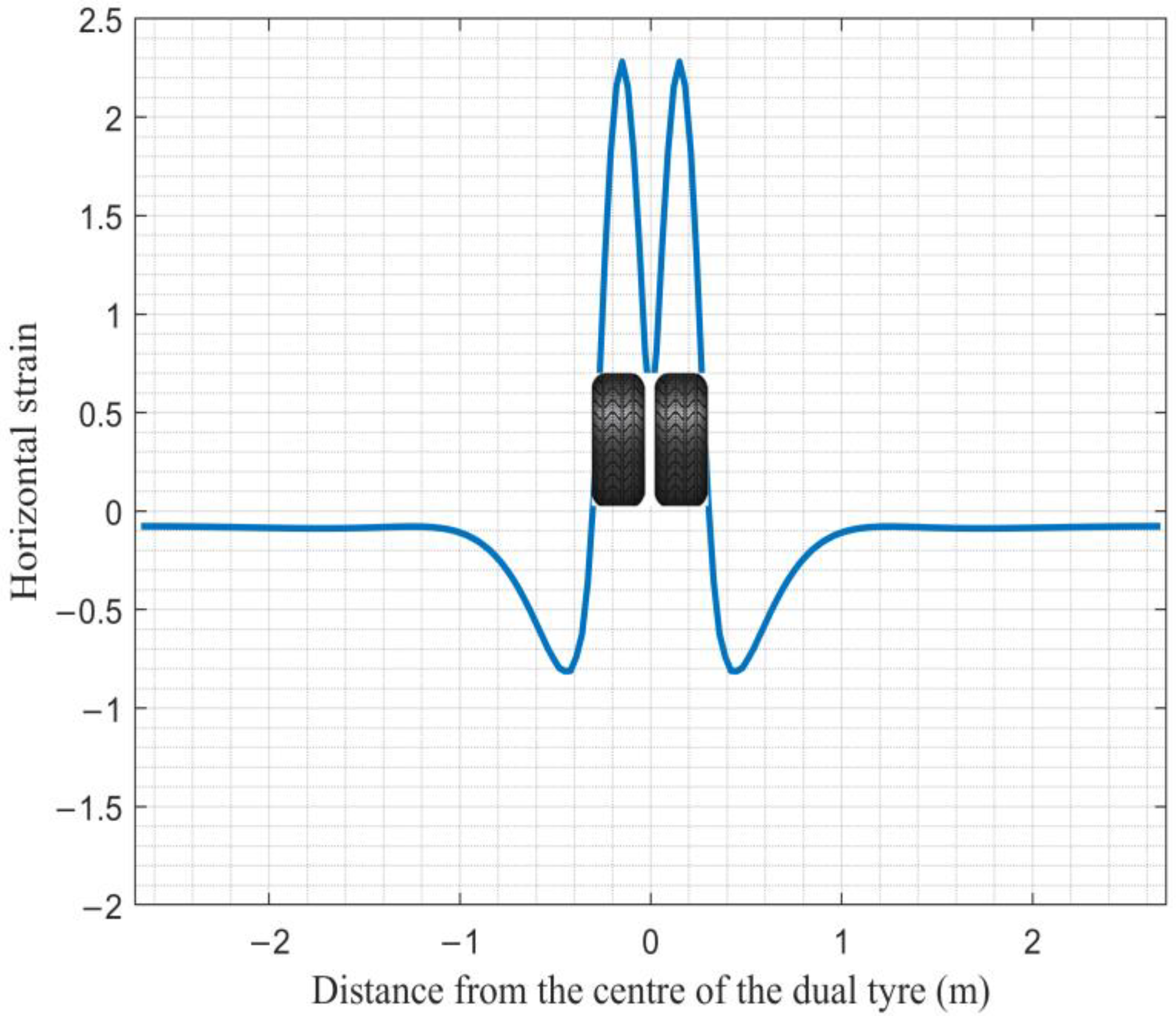
3.1.1. Horizontal Strain Distribution

The horizontal strain values at the bottom of the HMA layer for the 36 pavement cross-sections discussed above were determined. The strain distribution for the reference cross-section is presented in Figure 2 as an example. A positive value shows a tensile strain, and a negative value indicates a compressive strain. As discussed earlier in the paper, the critical strain values for causing fatigue damage in the HMA layer for the BU cases are determined by the maximum horizontal tensile strains experienced at the bottom of the layer. In this regard, as shown in Figure 2, the maximum horizontal tensile strain of $2.28{\left(10\right)}^{-4}$ was observed under the centre of the tyres for the reference pavement structure.

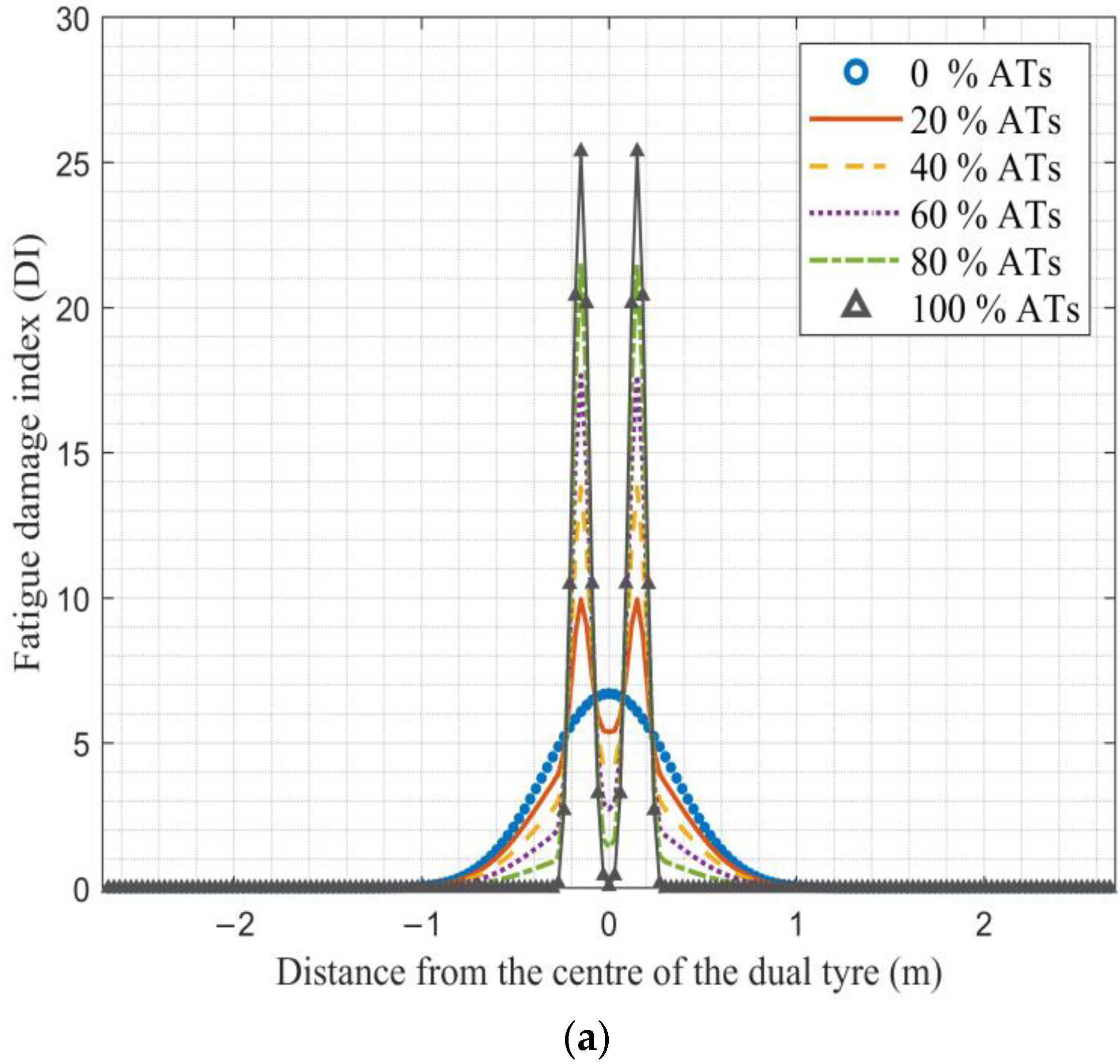
3.1.2. Fatigue Damage Index Distributions

By implementing the normal-wander mode for HDTs and zero- and uniform-wander mode for ATs for 30 million wheel passages, we calculated the transverse distribution of the total bottom-up damage index (BUDI) for the considered market penetration rates and lane widths. Considering the reference pavement structure, the individual effects of wander mode, market penetration, and lane width on the BUDIs is demonstrated in Figure 3, Figure 4 and Figure 5, respectively. In order to illustrate the impact of wander modes individually, we selected a lane width of 3.5 m and a market penetration rate of 100%. These values were chosen for illustrative purposes and to isolate the specific influence of wander modes on the results. Figure 3 shows the transverse distribution of the total BUDI for the scenarios with 100% AVs with zero- and uniform-wander and 100% HDTs with normal-wander modes. As seen in Figure 3, the maximum DI value for the zero-wander mode (i.e., 25.38) is 278.81% higher than for the normal-wander mode (i.e., 6.70) and 307.38% higher than for the uniform-wander mode (i.e., 6.23). It could also be observed that the maximum DI value in the uniform-wander case is 7.01% lower than the normal-wander one.

Subsequently, to demonstrate the effects of market penetration, we computed the DI values for the ATs’ different market penetration rates with zero- and uniform-wander modes combined with the HDTs with normal-wander mode, as shown in Figure 4. As can be seen, in the zero-wander mode, the maximum DI values are significantly increased by increasing the penetration rate. For instance, the maximum DI value in the case of 100% ATs (i.e., 25.38) is 155.32% higher than the case of 20% ATs (i.e., 9.94). In contrast, these values are decreased in the uniform-wander case. For instance, the maximum DI value in the case of 100% ATs (i.e., 6.23) is 5.75% lower than the case of 20% ATs (i.e., 6.61).

In the subsequent analysis, we compared the DI value distributions for a narrower lane width of 3 m with ones induced in the lane width of 3.5 m. As shown in Figure 5a, the maximum DI value for the normal-wander mode of HDTs for the lane width of 3 m (i.e., 7.61) is 13.58% higher than that for the lane width of 3.5 m (i.e., 6.70). In Figure 5b, the maximum DI value for the uniform-wander mode for the lane width of 3 m (i.e., 12.02) is 92.94% higher than that for the lane width of 3.5 m (i.e., 6.23). It should be noted that in the case of 100% ATs, the zero-wander mode is not influenced by the lane width because the zero vehicle frequency distribution of ATs is independent of the lane width. However, in the lower penetration rates of ATs, the existing HDTs’ normal-wander mode could be influenced by the lane width and consequently influence the DI value distributions.

3.2. Concise Comparative Analyses of Maximum Fatigue Damage Index

Considering the DI distribution scenarios discussed above, we determined and compared the maximum DI values presented in Figure 6. In the zero-wander mode cases, by increasing the ATs’ market penetration, the DI values increase for both the 3 m and 3.5 m lane widths. For these lane widths, the maximum BUDI values in the 100% ATs scenarios are 233% and 278% higher than in the 0% scenarios, respectively. In the uniform-wander mode cases, the effect of market penetration on the BUDI is influenced by the lane width. In this regard, by increasing the ATs’ penetration rate from 0% to 100%, the maximum BUDI values increase in the lane width of 3 m by around 58% and decrease in the lane width of 3.5 m by around 7%. As shown in Figure 6, considering a specific AT market penetration rate, the BUDI values in the uniform-wander mode are lower than the zero-wander modes in all penetration rates and both lane widths. However, the differences are more pronounced for the higher penetration rates. For instance, for lane widths of 3 m and 3.5 m, in the case of 20% ATs, the maximum BUDIs for the uniform-wander mode are 19% and 33.5% lower than the zero-wander mode, respectively. These difference values are about 52.6% and 75.4% for the case of 100% Ats, respectively.

3.3. Alternative Pavement Structures

To demonstrate the impact of increasing the layers’ thickness and stiffness on the fatigue damage induced by ATs, we computed the BUDI values for the three different surface thicknesses (i.e., 10 cm, 15 cm, and 20 cm), two base thicknesses (i.e., 20 cm and 40 cm), three surface elastic moduli (i.e., 9300 MPa, 6200 MPa, 3100 MPa), and two base moduli (i.e., 600 MPa and 300 MPa), as presented in Figure 7, Figure 8, Figure 9 and Figure 10, respectively. For all alternative pavement structures, we considered the lane widths of 3 m and 3.5 m, and we simulated the BUDI values for the zero- and uniform-wander modes with different penetration rates discussed earlier.

3.3.1. Layers’ Thickness Effect

As shown in Figure 7, in the zero-wander cases, increasing the thickness of the surface layer decreases the maximum BUDI value for all the penetration rates. It can be seen that the differences are more pronounced for the higher penetration rates. For instance, by increasing the thickness from 10 cm to 20 cm, the maximum BUDI value is decreased by 20.6% in the case of 20% ATs and by 42.9% in the case of 100% ATs. However, in the uniform-wander cases, the differences between BUDI values caused by increased thickness are less than 6.2% for all the penetration rates.

The impact of increased base thickness on the BUDI values is presented in Figure 8. In the zero-wander mode, increasing the thickness of the base layer from 20 cm to 40 cm resulted in a decrease of approximately 9.1% in the maximum BUDI values for the case of 20% ATs and 8.5% for the case of 100% ATs. In the uniform cases, the BUDI values have reductions ranging from 9.5% to 9.7% across all penetration rates.

The results presented in Figure 7 and Figure 8 provide insight into the influence of pavement layer thickness on the fatigue DI. These figures show that increasing surface and base layer thickness could reduce the maximum BUDI values in zero- and uniform-wander modes.

3.3.2. Layers’ Stiffness Effect

The effects of layers’ stiffness are demonstrated in Figure 9 and Figure 10. As shown in Figure 9, increasing the surface layer stiffness significantly decreases the maximum DI values in the zero-wander cases. The reduced DI values are more pronounced for the higher penetration rates. For instance, by increasing the stiffness of the surface layer from 3100 MPa to 9300 MPa, the maximum BUDI values are decreased by 26.6% for the case of 20% ATs and by 37.1% for the case of 100% ATs. Moreover, these differences are 17.7% and 19.4% in the uniform-wander case, respectively. This indicates that the reduced rate of fatigue DI values for different penetration rates are not considerably different in the uniform-wander cases.

In addition to the surface layer stiffness, increasing the base layer stiffness significantly decreases the maximum DI values, as shown in Figure 10. For instance, in the zero-wander cases, by increasing the base layer stiffness from 300 MPa to 600 MPa, the maximum BUDI values are decreased by 76.2% for the case of 20% ATs and 76.9% for the case of 100% ATs. These reduced percentage rates are 75.6% and 75.7% for the uniform-wander cases, respectively. The obtained results suggest that increasing the stiffness of the base layer yields a notable reduction in fatigue damage across all penetration rates and wander modes, including both zero-wander and uniform-wander scenarios. Nonetheless, it is noteworthy that the extent of damage reduction is not considerably different and is around 75.5% to 76.9%, respectively, both before and after the deployment of ATs on the roads.

3.3.3. Comparative Analyses of Layer’s Structure Effect on Fatigue DI Value

To demonstrate the comparative influence of thickness and stiffness variations in the surface and base layers on individual fatigue DI values, we selected a lane width of 3.5 m with a market penetration rate of 100% as an example. Figure 11 depicts the changes in fatigue DI values resulting from alterations in the thickness and stiffness of the surface and base layers when adopting 100% ATs under zero- and uniform-wander modes.

Upon a 100% increase in the thickness and stiffness of the layers, our findings reveal notable distinctions in the fatigue DI values. Under the zero-wander mode, the most substantial reduction in fatigue DI values occurs with increased base stiffness, followed by surface thickness, surface stiffness, and base thickness. Specifically, the fatigue DI values decreased by 77%, 43%, 24%, and 8%, respectively.

In the case of adopting the uniform-wander mode, the highest reductions in fatigue DI values are observed with an increase in base stiffness, surface stiffness, base thickness, and surface thickness, respectively. The corresponding reductions in fatigue DI values are 76%, 12%, 9%, and 6%, respectively.

3.3.4. Overview of Fatigue Damage Index Variations across Evaluated Scenarios

Table 2. Percentage changes in DI values.

Lane Width	3 m				3.5 m
Scenario	Integrated		Segregated		Integrated		Segregated
Market Penetration Rate	20% to 80%		100%		20% to 80%		100%
Wander Mode of ATs	Zero	Uniform	Zero	Uniform	Zero	Uniform	Zero	Uniform
Percentage Change of DI Compared to the Reference Scenario (0% ATs)	+37.67% to +184%	+11.6% to +46.41%	+233.57%	+58.01%	+48.29% to +221%	−1.41% to −5.64%	+278.57%	−7.05%
Aggravator/Mitigator	Aggravator	Aggravator	Aggravator	Aggravator	Aggravator	Mitigator	Aggravator	Mitigator
Reduced Percentage of DI by Increasing the HMA Layer’s Thickness from 10 cm to 20 cm	−17.59% to −40.04%	−0.06% to −1.44%	−42.92%	−1.76%	−20.58% to −40.43%	NA *	−42.92%	NA
Reduced Percentage of DI by Increasing the Base Layer’s Thickness from 20 cm to 40 cm	−9.10% to −8.58%	−9.82% to −9.95%	−8.51%	−9.98%	−9.06% to −8.51%	NA	−8.51%	NA
Reduced Percentage of DI by Increasing the HMA Layer’s Stiffness from 3100 MPa to 9300 MPa	−25.32% to −35.87%	−16.26% to −16.24%	−37.90%	−16.23%	−26.62% to −36.01%	NA	−37.09%	NA
Reduced Percentage of DI by Increasing the Base Layer’s Stiffness from 300 MPa to 600 MPa	−76.20% to −76.8%	−75.51% to −75.55%	−76.88%	−75.55%	−76.24% to −76.81%	NA	−76.88%	NA

* Not applicable: since the DI values are not higher in the mitigator scenarios than in the human-driven vehicles’ situation, no thickness or stiffness design change is necessary.

provides an overview of the variations in the DI values across different scenarios. In this table, the comparisons of DI values are presented by percentage changes in the fatigue damage index, which serve as indicators, offering insights into the potential trends of increased or decreased fatigue damage within specific scenarios. Since the direct interpretation and utilisation of fatigue damage alteration magnitudes may be limited, our analysis focuses on discerning trends in these alterations. In other words, rather than solely focusing on absolute fatigue damage index values, our study emphasises the comparative patterns observed across diverse scenarios. By examining the relative changes in fatigue damage, the present study aimed to elucidate the influence of various parameters, including wandering patterns, lane widths, market penetration rate, and pavement layer thicknesses and stiffnesses. Therefore, the magnitudes of alterations may not be interpreted and employed directly; instead, the observed trends are more informative.

According to the results presented in Table 2, the scenarios reveal significant variations in DI depending on the lane width (3 m vs. 3.5 m), market penetration rates (ranging from 20% to 100%), and wander modes (zero vs. uniform). For instance, a segregated scenario with a 3.5 m lane width and zero wander at a 100% market penetration rate shows a substantial increase in the DI by 278.57%, indicating aggravated fatigue damage. Conversely, the same scenario with uniform wander demonstrates mitigator fatigue damage with a decrease in DI by 7.05%.

Furthermore, Table 2 highlights the effectiveness of various pavement alternative structures in reducing the DI. Increasing the HMA layer’s thickness from 10 cm to 20 cm shows a notable reduction in the DI, particularly in zero-wander scenarios with higher AT penetration rates. For example, a segregated scenario with 100% penetration and zero wander reduces the DI by 42.92% with the increased HMA layer thickness. Similarly, increasing the base layer’s stiffness from 300 MPa to 600 MPa consistently reduces the DI across all evaluated scenarios, with reductions exceeding 75%.

Overall, Table 2 illustrates the critical impact of traffic integration, lane width, and pavement layer modifications on fatigue damage. It underscores the importance of strategic pavement design and traffic management to mitigate fatigue damage and prolong pavement life.

4. Discussion

The simulation results in this study present various quantitative comparisons between the fatigue damage incurred by distinct pavement structures that have undergone exposure to the normal-wander mode of HDTs mixed with the zero- and uniform-wander modes of ATs, considering different market penetrations and lane widths. These comparisons offer several insights that can provide practical considerations regarding the impact of AT deployment scenarios compared with the non-AT scenarios and identify the cases that could lead to accelerated fatigue damage in the long term.

Furthermore, this research provides practical suggestions, such as improving layers’ thickness and stiffness to mitigate the adverse effects of increased damage and alleviate potential challenges associated with AT deployment. In other words, comparing different pavement structures subjected to different load distribution scenarios revealed significant differences in the fatigue damage incurred by the pavements. This suggests that pavement designers and managers should consider the ATs’ penetration rate and wander patterns when selecting appropriate lane widths or pavement materials and thicknesses in their designs. The subsequent sections discuss the present study’s findings and their implications.

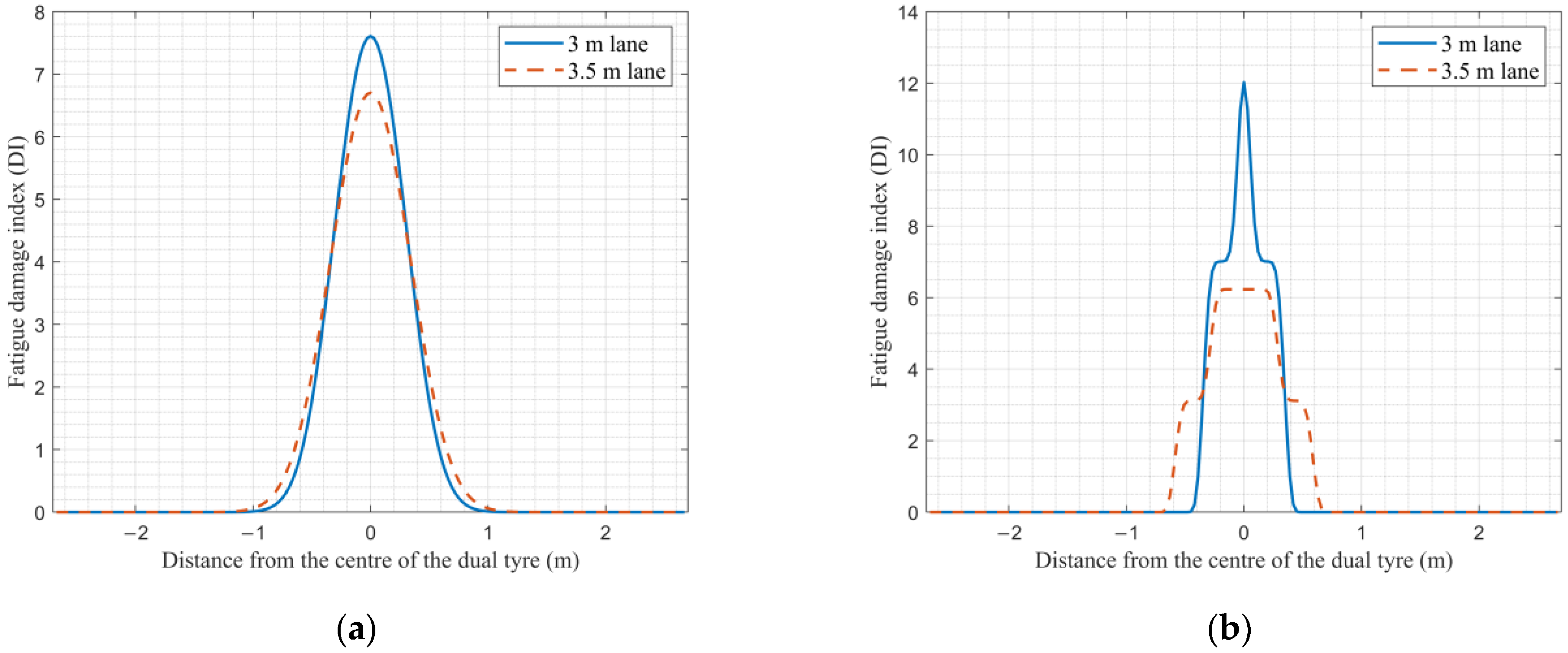
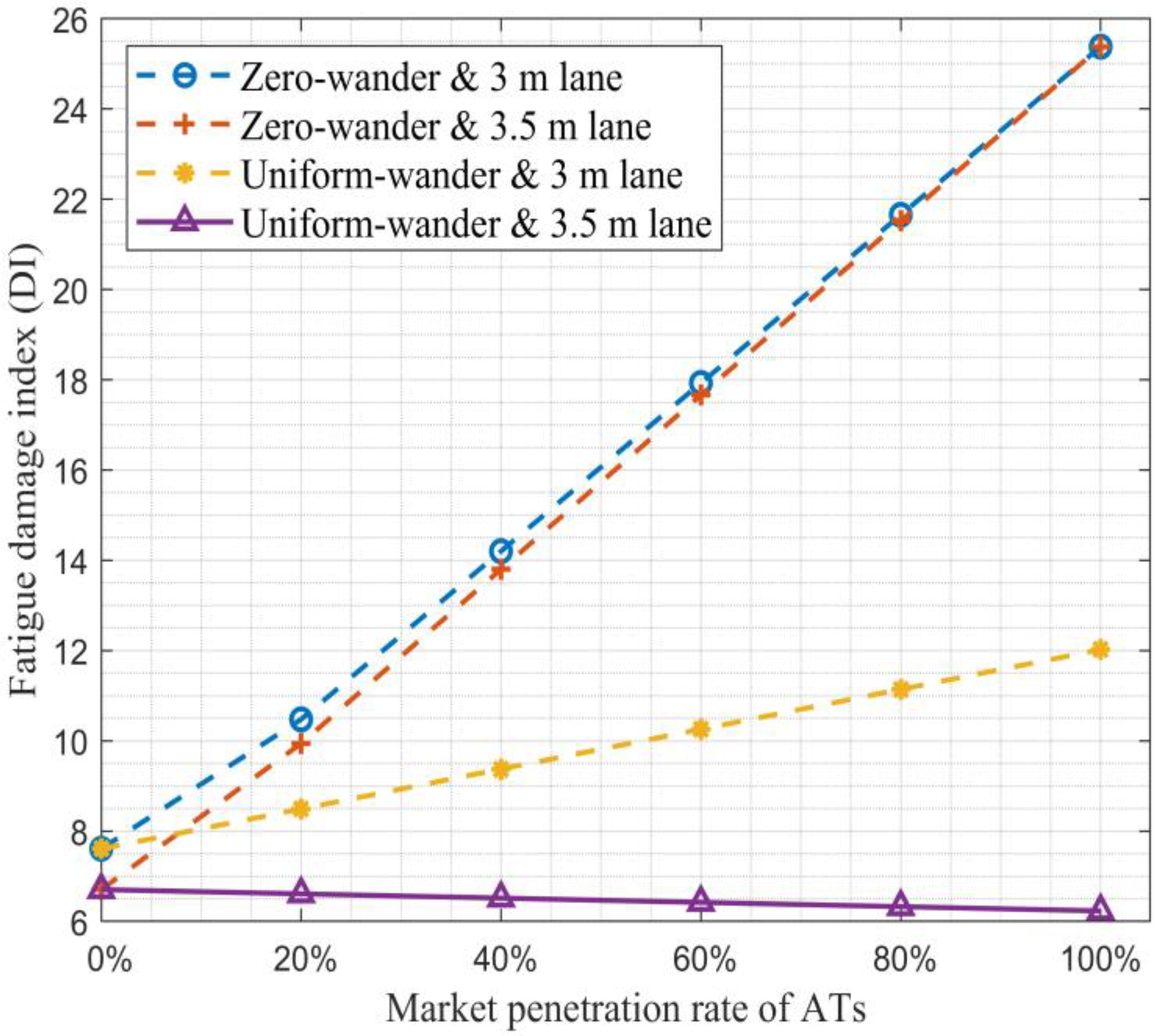
• Comparing the DI values resulting from the introduction of ATs on roads to scenarios featuring only HDTs revealed that AT deployment could either decrease the fatigue DI (i.e., ‘DI mitigator scenarios’) or increase it (i.e., ‘DI aggravator scenarios’), depending on the AT deployment scenarios. For instance, in the case of adopting a uniform-wander mode for ATs on a 3.5 m wide lane, the deployment of ATs does not negatively impact pavement fatigue performance compared to the non-AT scenarios. In contrast, it may even slightly decrease the DI values. This reduction is more considerable in the segregated scenarios than in the integrated ones. This finding is in agreement with the findings of Chen et al. [16], indicating that in the worst-case scenario where only zero-wander-distributed trucks are on the pavement, the fatigue damage is 2.7 times that of human-driven trucks. Conversely, for other lateral control modes, higher proportions of autonomous trucks result in less fatigue damage, extending pavement life.
• The findings of this study support the previous findings of Noorvand et al. [15] and Zhou et al. [17], recommending the use of uniform-wander mode for ATs compared to zero-wander mode. In addition, these findings recommend using segregated lane distribution together with the uniform-wander mode only if wider lanes (e.g., 3.5 m) are present in the era of AT deployment, in order to further reduce pavement fatigue damage in the long term (see Table 2).
• The aggravator scenarios are observed using a narrower lane of 3 m in both zero- and uniform-wander cases and in the lane width of 3.5 m only when the zero-wander mode is implemented. This is in line with the findings of Chen et al. [16], indicating that autonomous trucks’ lateral distribution increases fatigue damage at the bottom of the asphalt layer compared to traditional trucks, emphasising the need for proper lateral control to mitigate this impact. Comparing the DI values of different market penetrations revealed that the increased DI values of AT scenarios are more pronounced in the higher market penetrations than the lower ones and in the zero-wander scenarios than the uniform-wander ones. Chen et al. [16] also argued that the damage increases with a higher proportion of ATs.
• Although using the uniform-wander mode could result in lower fatigue damage than the zero-wander mode, this could still cause more damage than the non-AT scenarios for the narrower lane of 3 m. Thus, in the DI aggravator scenarios, the increased fatigue damage percentages induced by ATs are considerable, and further actions, such as increasing the thickness or stiffness of the layers, should be performed to mitigate their negative impact on pavement fatigue performance.
• A practical implication for lane distribution management is recommending integrated lane distributions for ATs (i.e., compared with segregated cases) in the DI aggregator scenarios. This could reduce the adverse negative impact of AT deployment on pavement fatigue.
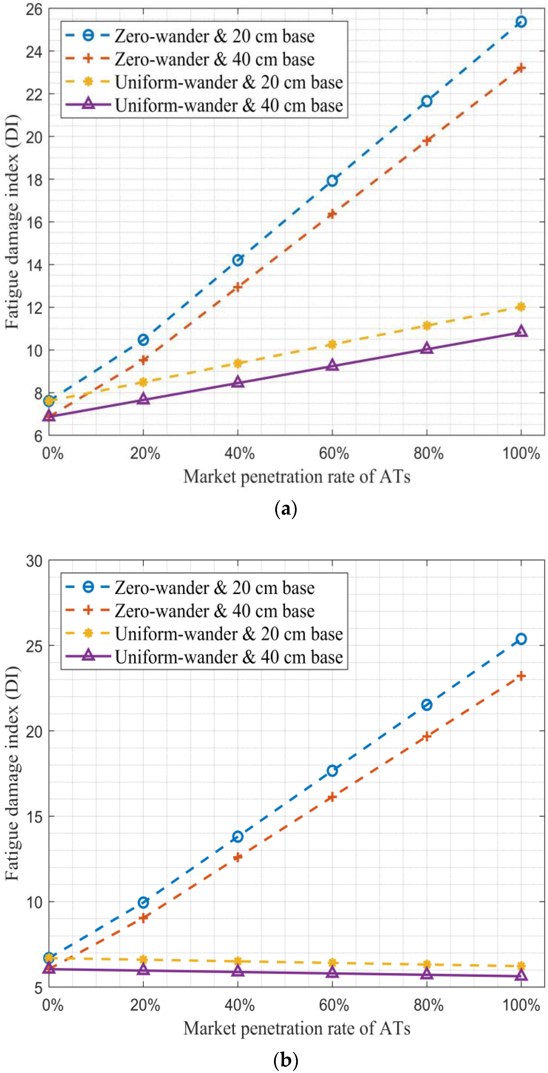
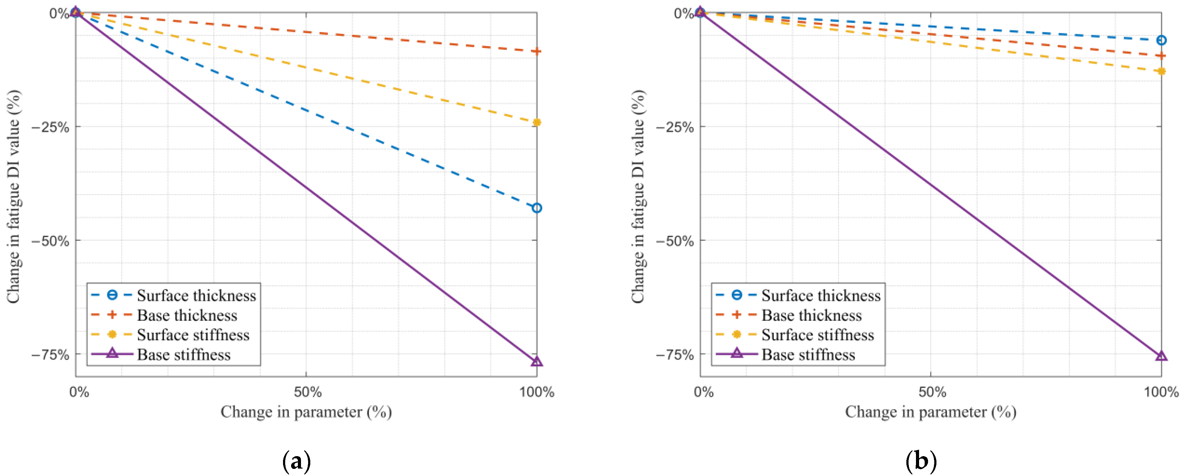
• Comparing the effect of increased surface layer thickness and base layer thickness on the reduced percentages of DI values (see Table 2) revealed a practical implication that the use of a thicker surface layer could be more effective in mitigating the ATs’ negative impact on pavement fatigue damage than the use of a thicker base layer for the zero-wander mode (see Figure 11a). In contrast, when using the uniform-wander mode, the observed results are the other way around, meaning that the thicker base layer could be more effective in reducing fatigue damage (see Figure 11b). However, an economic analysis study is needed to compare the costs of increasing the surface and base layer thickness and the benefits of prolonging the pavement life and reduced maintenance costs obtained from each DI mitigation solution.
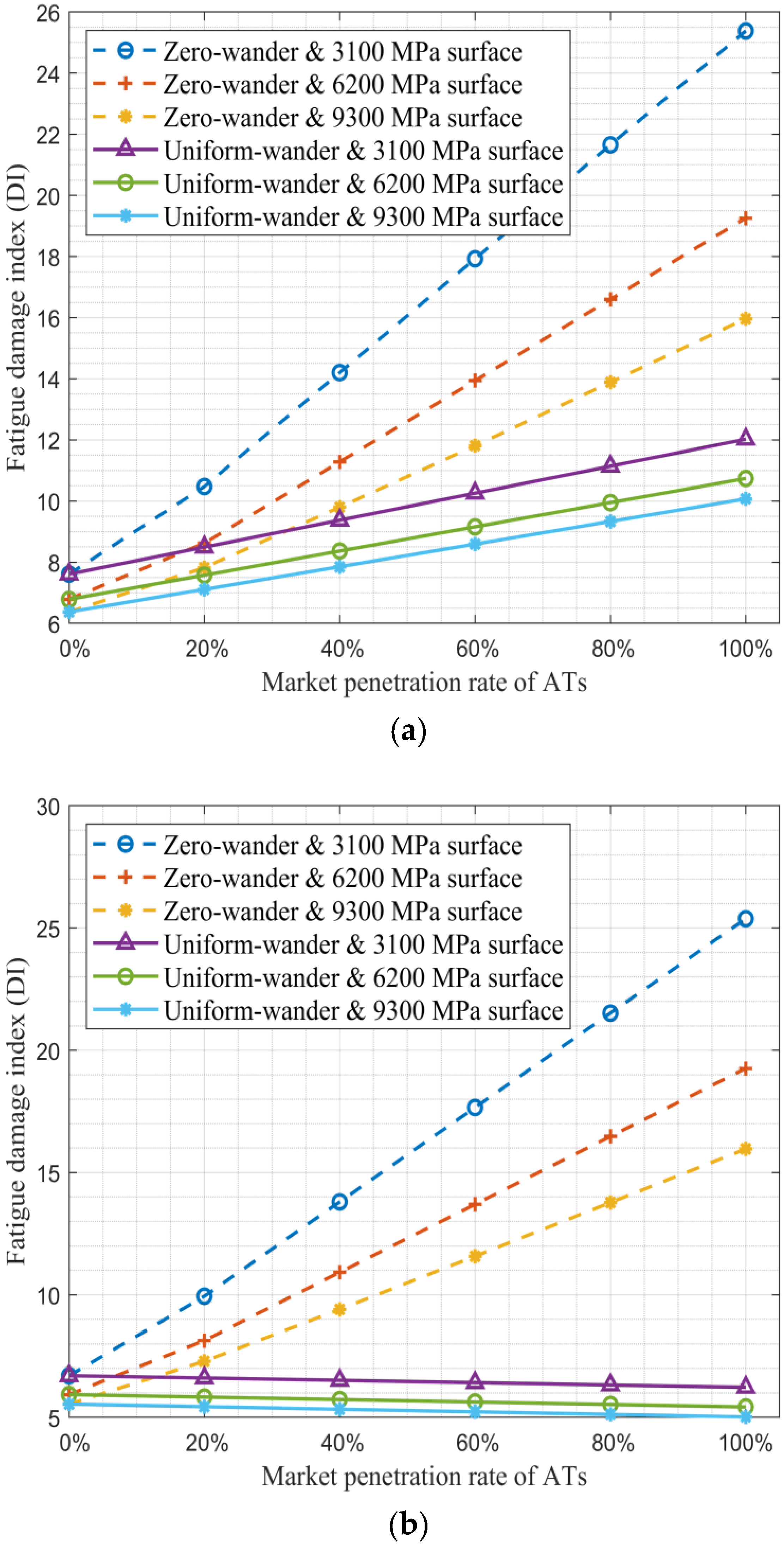
• Increasing the stiffness of the surface and base layer could result in reduced maximum DI values for the zero-wander mode, with more pronounced differences in the higher penetration rates. These results indicate that the stiffness of the base and surface layer plays a crucial role in mitigating the impact of ATs’ wander mode on the pavement’s fatigue performance. Notably, the reduced rates of maximum DI values caused by an increased surface layer stiffness are significantly lower for the uniform-wander mode compared to the zero-wander mode. Furthermore, in agreement with the findings of Georgouli et al. [8], the present study showed that the increased thickness of the HMA layer has a more significant impact on reducing fatigue damage than its stiffness for the zero-wander mode cases (see Figure 11a).
• The reduced percentage rates of maximum BUDI values caused by increased base layer stiffness are around 75.51% to 76.88% in all the penetration rates, which indicates that the effect of base layer stiffness on fatigue performance is consistent across different levels of market penetration rates, and is consistently higher compared to the impact of surface layer thickness increase (see Figure 11). These results suggest that investing in higher base layer stiffness could be a promising strategy to mitigate the negative impacts of ATs’ wander mode on the pavement’s fatigue performance in all the penetration rates in the aggravator scenarios.

Limitations and Future Research

It is also essential to acknowledge a few limitations of the current study. The present study used numerical simulations using a specific tyre–pavement interaction and load model, which may not represent all possible tyre–pavement conditions. The accuracy of the results depends on the accuracy of the model assumptions, including the pavement layers’ material properties and the load model. Therefore, the results of this study should be validated using experimental data from field tests or laboratory experiments. Furthermore, the present study used Miner’s rule to compute fatigue damage, which assumes linear damage accumulation. This may not always be accurate in real-world situations. Additionally, Miner’s rule does not account for variations in loading frequencies or amplitudes and the possibility of crack growth and propagation, which can affect the accumulated fatigue damage. Moreover, the present study focused only on the BU fatigue damage. Thus, investigating top–down fatigue damage could further corroborate the current understanding of pavement fatigue performance influenced by ATs.

The findings highlight the complex and interdependent factors affecting pavement’s fatigue performance under different AT deployment scenarios. This necessitates further research to investigate the other potential AT deployment scenarios affecting pavement fatigue damage.

In addition to the limitations discussed above, it is imperative to recognise the need for a comprehensive evaluation of the integration of our findings with other pavement failure modes and distresses. This broader perspective will provide a more holistic understanding of pavement performance under varying AT scenarios. Furthermore, to enhance the practical applicability of our research, a thorough economic appraisal of interventions, such as modifying pavement thickness, width, or stiffness, is essential. These considerations are pivotal for offering cost-effective and sustainable solutions.

5. Conclusions

In this study, we numerically simulated the fatigue performance of 864 unique scenarios with varying wander modes, market penetration, lane width, and flexible pavement layers’ thickness and stiffness. The fatigue damage index (DI) for each scenario was calculated and compared to understand the impacts of these variables on pavement fatigue. In summary, our study’s findings yield practical recommendations for vehicle designers and road practitioners. During the initial stages of AT implementation, characterised by low market penetration, we advise using the uniform-wander mode over the zero-wander mode to mitigate ATs’ negative impact on pavement fatigue damage. Additionally, in the full automation era, utilising wider lanes can further safeguard against increased fatigue damage associated with ATs. However, if truck manufacturers are compelled to adopt the default zero-wander mode, the efficacy of wider lanes diminishes in terms of fatigue damage reduction. Instead, enhancing pavement layer stiffness or thickness from the outset becomes imperative. Alternatively, dedicating narrower lanes may offer cost savings without significantly exacerbating fatigue damage. Nonetheless, a comprehensive economic analysis and further investigation are requisite to thoroughly assess the associated costs and benefits.

References

1. Gungor, O.E.; Al-Qadi, I.L. All for one: Centralized optimization of truck platoons to improve roadway infrastructure sustainability. Transp. Res. Part C Emerg. Technol. 2020, 114, 84–98. [Google Scholar] [CrossRef]
2. Gungor, O.E.; Al-Qadi, I.L. Wander 2D: A flexible pavement design framework for autonomous and connected trucks. Int. J. Pavement Eng. 2020, 23, 121–136. [Google Scholar] [CrossRef]
3. Chen, F.; Song, M.; Ma, X. A lateral control scheme of autonomous vehicles considering pavement sustainability. J. Clean. Prod. 2020, 256, 120669. [Google Scholar] [CrossRef]
4. Song, M.; Chen, F.; Ma, X. Organization of autonomous truck platoon considering energy saving and pavement fatigue. Transp. Res. Part D Transp. Environ. 2020, 90, 102667. [Google Scholar] [CrossRef]
5. Srisomboon, I.; Lee, S. Efficient position change algorithms for prolonging driving range of a truck platoon. Appl. Sci. 2021, 11, 10516. [Google Scholar] [CrossRef]
6. Lee, S.; Cho, K.; Park, H.; Cho, D. Cost-Effectiveness of Introducing Autonomous Trucks: From the Perspective of the Total Cost of Operation in Logistics. Appl. Sci. 2023, 13, 10467. [Google Scholar] [CrossRef]
7. Kim, J. Truck platoon control considering heterogeneous vehicles. Appl. Sci. 2020, 10, 5067. [Google Scholar] [CrossRef]
8. Georgouli, K.; Plati, C. Autonomous trucks’ (ATs) lateral distribution and asphalt pavement performance. Int. J. Pavement Eng. 2022, 24, 2046274. [Google Scholar] [CrossRef]
9. Yeganeh, A.; Vandoren, B.; Pirdavani, A. Pavement rutting performance analysis of automated vehicles: Impacts of wander mode, lane width, and market penetration rate. Int. J. Pavement Eng. 2023, 24, 2049264. [Google Scholar] [CrossRef]
10. Pais, J.; Pereira, P.; Thives, L. Wander Effect on Pavement Performance for Application in Connected and Autonomous Vehicles†. Infrastructures 2023, 8, 119. [Google Scholar] [CrossRef]
11. Othman, K. Impact of autonomous vehicles on the physical infrastructure: Changes and challenges. Designs 2021, 5, 40. [Google Scholar] [CrossRef]
12. Guo, R.; Liu, S.; He, Y.; Xu, L. Study on Vehicle–Road Interaction for Autonomous Driving. Sustainability 2022, 14, 11693. [Google Scholar] [CrossRef]
13. Severino, A.; Curto, S.; Barberi, S.; Arena, F.; Pau, G. Autonomous vehicles: An analysis both on their distinctiveness and the potential impact on urban transport systems. Appl. Sci. 2021, 11, 3604. [Google Scholar] [CrossRef]
14. Chen, F.; Balieu, R.; Kringos, N. Potential Influences on Long-Term Service Performance of Road Infrastructure by Automated Vehicles. Transp. Res. Rec. J. Transp. Res. Board 2016, 2550, 72–79. [Google Scholar] [CrossRef]
15. Noorvand, H.; Underwood, B.S. Autonomous Vehicles: Assessment of the Implications of Truck Positioning on Flexible Pavement Performance and Design. Transp. Res. Rec. 2017, 2640, 21–28. [Google Scholar] [CrossRef]
16. Chen, F.; Song, M.; Ma, X.; Zhu, X. Assess the impacts of different autonomous trucks’ lateral control modes on asphalt pavement performance. Transp. Res. Part C Emerg. Technol. 2019, 103, 17–29. [Google Scholar] [CrossRef]
17. Zhou, F.; Hu, S.; Chrysler, S.T.; Kim, Y.; Damnjanovic, I.; Talebpour, A.; Espejo, A. Optimization of Lateral Wandering of Automated Vehicles to Reduce Hydroplaning Potential and to Improve Pavement Life. Transp. Res. Rec. 2019, 2673, 81–89. [Google Scholar] [CrossRef]
18. Rana, M.M.; Hossain, K. Simulation of autonomous truck for minimizing asphalt pavement distresses. Road Mater. Pavement Des. 2021, 23, 1266–1286. [Google Scholar] [CrossRef]
19. Georgouli, K.; Plati, C.; Loizos, A. Autonomous vehicles wheel wander: Structural impact on flexible pavements. J. Traffic Transp. Eng. 2021, 8, 388–398. [Google Scholar] [CrossRef]
20. Chen, L.; Chen, D.; Chen, C.; Jiang, X.; Liu, L. Dynamic Impact Analysis of Automated Bus on Asphalt Pavement. In Proceedings of the 3rd International Forum on Connected Automated Vehicle Highway System through the China Highway & Transportation Society, Jinan, China, 23–25 October 2020. [Google Scholar] [CrossRef]
21. Yeganeh, A.; Vandoren, B.; Pirdavani, A. The Effects of Automated Vehicles Deployment on Pavement Rutting Performance. In Airfield and Highway Pavements; American Society of Civil Engineers (ASCE): Reston, VA, USA, 2021; pp. 280–292. [Google Scholar] [CrossRef]
22. Merhebi, G.H.; Joumblat, R.; Elkordi, A. Assessment of the Effect of Different Loading Combinations Due to Truck Platooning and Autonomous Vehicles on the Performance of Asphalt Pavement. Sustainability 2023, 15, 10805. [Google Scholar] [CrossRef]
23. Tian, G.; Jia, Y.; Chen, Z.; Gao, Y.; Wang, S.; Wei, Z.; Chen, Y.; Zhang, T. Evaluation on Lateral Stability of Vehicle: Impacts of Pavement Rutting, Road Alignment, and Adverse Weather. Appl. Sci. 2023, 13, 3250. [Google Scholar] [CrossRef]
24. Ma, X.; Shangguan, L.; Si, C. Probability Distributions of Asphalt Pavement Responses and Performance under Random Moving Loads and Pavement Temperature. Appl. Sci. 2023, 13, 715. [Google Scholar] [CrossRef]
25. Yeganeh, A.; Vandoren, B.; Pirdavani, A. Impacts of Load Distribution and Lane Width on Pavement Rutting Performance for Automated Vehicles. Int. J. Pavement Eng. 2021, 23, 4125–4135. [Google Scholar] [CrossRef]
26. Hayeri, Y.M.; Hendrickson, C.; Biehler, A.D. Potential impacts of vehicle automation on design, infrastructure and investment decisions-a state dot perspective. In Proceedings of the Transportation Research Board 94th Annual Meeting, Washington, DC, USA, 11–15 January 2015. [Google Scholar]
27. Heinrichs, D. Autonomous driving and urban land use. In Autonomous Driving; Springer: Cham, Switzerland, 2016; pp. 213–231. [Google Scholar]
28. Machiani, S.G.; Ahmadi, A.; Musial, W.; Katthe, A.; Melendez, B.; Jahangiri, A. Implications of a Narrow Automated Vehicle-Exclusive Lane on Interstate 15 Express Lanes. J. Adv. Transp. 2021, 2021, 6617205. [Google Scholar] [CrossRef]
29. Hafiz, D.; Zohdy, I. The City Adaptation to the Autonomous Vehicles Implementation: Reimagining the Dubai City of Tomorrow. In Towards Connected and Autonomous Vehicle Highways; Springer: Berlin/Heidelberg, Germany, 2021; pp. 27–41. [Google Scholar]
30. McCullah, J.; Gray, D. National Cooperative Highway Research Program. 2005, Volume 10. Available online: https://onlinepubs.trb.org/onlinepubs/nchrp/nchrp_rpt_480.pdf (accessed on 28 May 2024).
31. Coca, A.M.; Romanoschi, S.A.; Talebsafa, M.; Popescu, C. Simple Method for Incorporating Lateral Wheel Wander in the Computation of Fatigue Damage in New Flexible Pavement Structures. J. Transp. Eng. Part B Pavements 2020, 146, 04020074. [Google Scholar] [CrossRef]
32. Canestrari, F.; Ingrassia, L.P. A review of top-down cracking in asphalt pavements: Causes, models, experimental tools and future challenges. J. Traffic Transp. Eng. 2020, 242, 118043. [Google Scholar] [CrossRef]
33. Smith, M. ABAQUS/Standard User’s Manual, Version 6.9; Dassault Systèmes Simulia Corp.: Providence, RI, USA, 2009. [Google Scholar]
34. Buiter, R.; Cortenraad, W.M.H.; van Eck, A.C.; van Rij, H. Effects of transverse distribution of heavy vehicles on thickness design of full-depth asphalt pavements. Transp. Res. Rec. 1989, 1227, 66–74. [Google Scholar]
Figure 1. Flowchart depicting the sequential steps undertaken in the research methodology.
Applsci 14 05552 g001
Figure 2. Horizontal strain values for the reference cross-section at the bottom of the HMA layer.
Applsci 14 05552 g002
Figure 3. DI value distributions for different wander modes for BUDI.
Applsci 14 05552 g003
Figure 4. DI value distributions for the different penetration rates for the (a) zero-wander mode and (b) uniform-wander mode.
Applsci 14 05552 g004aApplsci 14 05552 g004b
Figure 5. DI values for the different lane widths for 100% HDTs (a) with normal-wander and (b) with uniform-wander modes.
Applsci 14 05552 g005
Figure 6. Maximum DI values of zero- and uniform-wander distributions with different penetration rates for lane widths of 3 m and 3.5 m.
Applsci 14 05552 g006
Figure 7. DI values for the different surface thicknesses for lane widths of (a) 3 m and (b) 3.5 m.
Applsci 14 05552 g007
Figure 8. DI values for the different base thicknesses for lane widths of (a) 3 m and (b) 3.5 m.
Applsci 14 05552 g008
Figure 9. DI values for the different surface stiffnesses for lane widths of (a) 3 m and (b) 3.5 m.
Applsci 14 05552 g009
Figure 10. DI values for the different base stiffnesses for lane widths of (a) 3 m and (b) 3.5 m.
Applsci 14 05552 g010
Figure 11. Changes in fatigue DI values by changing layers’ structure by applying 100% ATs with (a) zero-wander and (b) uniform-wander modes.
Applsci 14 05552 g011