Abstract
The study aimed to evaluate for the first time the degree of contamination of soil and crops with major and trace elements (Cd, Co, Cr, Cu, Ni, Pb, Zn, F, Na, Mg, Si, P, Cl, Fe, Al) in agricultural lands situated in the Lower Danube Basin, Galati and Braila counties (SE Romania), impacted by the steel industry. Soil samples, as well as leaves and seeds of wheat, corn, and sunflower, were collected from two depths in 11 different sites. Along with elemental and mineralogical analyses, performed by HR-CS AAS, PIGE, SEM-EDX, and ATR-FTIR, the soil pH, texture, organic matter, electric conductivity, and CaCO3 content were investigated. The results showed that the levels of Cr (83.27–383.10 mg kg−1), Cu (17.11–68.15 mg kg−1), Ni (30.16–55.66 mg kg−1), and F (319–544 mg kg−1) in soil exceeded the Romanian regulations for sensitive use of the land. Igeo, EF, PI, and PERI pollution indices indicate that the soil is moderate to highly contaminated with Cr, Ni, and Cu, while the CSI and mERMQ indices suggested a relatively low risk for metal contamination. The elemental concentrations in plant tissues and bioaccumulation factors (BFs) provide valuable insights into the soil–plant relationship, health risks, and the selectivity of plant compartments for different elements. Thus, the results revealed that the wheat plants tended to exclude the bioaccumulation of particular elements in their tissues, while exhibiting a different bioaccumulation pattern for Zn and Cu. In the case of corn, most BFs were below one, indicating a limited phytoaccumulation capacity. However, exceptions were observed for Cd, Zn, and Cu with the sunflower BFs indicating higher bioconcentration of these elements in leaves and seeds compared to other elements. Chromium (Cr) contributes to non-carcinogenic dermal contact and ingestion hazards, children being more susceptible to the adverse effects of this contaminant.
Keywords:
soil; wheat; sunflower; corn; trace elements; pollution; heavy metals; bioaccumulation factor; Lower Danube Basin; health risk 1. Introduction
The responsible and judicious management of soil resources is of paramount importance in maintaining the sustainability of our environment. This includes the utilization of appropriate practices for the preservation and protection of soil health and fertility, while also taking into account the unique characteristics of each specific soil type [1]. The soil is a critical natural resource that plays a vital role in sustaining life on Earth. It serves as an interface between different geospheres and interacts with them to exchange matter and energy. Numerous studies have demonstrated the ecological significance of soil, with edaphic conditions directly influencing the chemical composition and plant growth [2,3,4]. Soils in proximity to industrial areas, heavily trafficked roads, mines, and waste storage centers are exposed to high levels of elements and toxic chemical compounds. These contaminants can disrupt natural biological processes and may be absorbed by plants, subsequently entering the food chain [5,6,7,8]. Furthermore, the fertilizers and pest control products can harm the soil by elements they contain, posing additional risks to the ecosystem.
The issue of environmental pollution in Galati and Braila counties, Lower Danube Basin, SE Romania, is a significant concern, particularly due to the long period of industrial activities of the Galati Steel Enterprise. The steel plant began production 65 years ago, which led to the neighboring lands’ contamination with toxic elements, mostly heavy metals (HMs) [9]. Although plant re-engineering has helped in reducing emissions, the irrational use of chemical fertilizers and pesticides still causes significant imbalances in the adjacent agroecosystems. To increase crop production and plants’ resistance to pests and diseases, farmers use large amounts of fertilizers (chemical, organic, and sewage sludges) and pesticides, which pose significant risks to the ecosystem due to harmful elements entering the soil. These elements, including HMs (Ni, Cr, Zn, Cd, Cu, As) and toxic chemicals (insecticides, herbicides, fungicides), can leach into the soil through runoff or direct absorption [10]. Negative effects may occur on soil quality, harming the biota (microorganisms, plants, animals, and humans) and even contaminating groundwater. The long-term consequences of soil contamination are far-reaching, potentially affecting agricultural productivity and human health. For instance, crops grown in contaminated soil can absorb harmful elements, which may have detrimental effects when consumed. Furthermore, exposure to dispersed soil particles through inhalation, ingestion, or dermal contact can increase the risk of developing various diseases. If contaminants are present in the environment, they can contribute to both acute and chronic health issues, including conditions such as renal impairment, osteoporosis [11], mitochondrial dysfunction and associated diseases [12], lung carcinoma [13], and cardiovascular disorder [14].
Currently, there are limited data on soil contamination with HMs caused by steelmaking or other human activities in the Galati–Braila region [9]. Regarding the contamination of cultivated plants, vegetables, fruits, and fodder plants with toxic elements discharged from industrial activities, as well as the mismanagement of fertilizers, amendments, and pesticides, there are a lack of specific data for the area under investigation.
The main objective of this study was to examine the extent of soil and crop (wheat, corn, sunflower) contamination with both major and trace elements in the industrial area of Galati metallurgical enterprise. These elements are crucial for supporting life on Earth, but their presence at elevated levels can pose considerable health risks. The study also aimed to determine the elemental bioaccumulation in crop tissues and to assess the contamination level and risk of toxic elements in soils using pollution indices and the human health hazards associated with ingestion, dermal contact, and inhalation of the toxicants. It is worth mention that the present study constitutes the first detailed exploration of this specific subject in the Lower Danube region, Galati–Braila area.
2. Materials and Methods
2.1. Study Area
The research was carried out in three administrative territorial units (AUTs) from the south of Galati (GL) County (Tulucesti (TUL) and Sendreni (SEN)) and north of Braila (BR) County (Vadeni (VAD)), southeast of Romania, in some agricultural territories from the Lower Danube Basin, which are near the Iron and Steel Plant (I.S.P.) industry (Figure 1) [1]. This area is geographically located in the Covurlui and Siret Plains and is characterized by quaternary loess and loessoid deposits of eolian origin, as well as fluviatile deposits. These deposits are the parent material for the prevalent soil types in this area, namely chernozems and fluvisols.
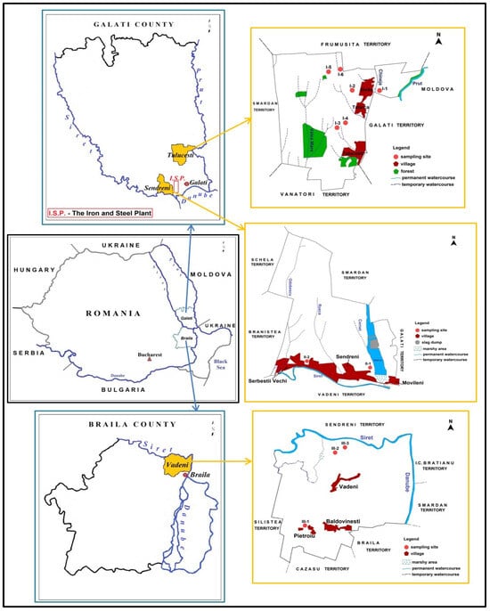
Figure 1.
Soil and crop collection sites in Tulucesti, Sendreni, and Vadeni, Galati–Braila region, SE Romania.
The sampling sites were located on arable lands, cultivated with the three main crops that have the highest favorability for the researched area, namely Triticum vulgare Vill. (wheat), Zea mays L. (corn), and Helianthus annuus L. (sunflower). The position of the collection sites is presented in Table 1.

Table 1.
The geographical position of soil sampling sites.
2.2. Soil Sampling and Plant Collection
The soil samples were collected with a stainless-steel knife from pits that measured 30 × 30 × 30 cm, divided into two depth sections (the first section up to 5 cm and the second one up to 30 cm depth), according to [15]—Figure 2. Each soil sample, weighing approximately 400 g, was carefully stored in a hermetically sealed plastic bag, which was labeled for identification purposes. To prevent contamination from the top layer, the samples were collected from the bottom upwards. The depths were defined, and the excavation site was refreshed before sampling.
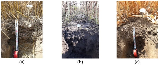
Figure 2.
Soil sampling pits from crop allotments: (a) wheat, (b) sunflower (c) corn.
The crop samples were made up of mature and healthy plants from the same areas where the soil was taken. The sampling process was carried out following the guidelines provided by [16]. During the sampling process, plants located at the ends of the lots and visibly affected ones were excluded.
2.3. Soil and Plant Analysis
The soil samples were cleaned of roots, stones, and other debris, air-dried, crushed in a porcelain mortar, and sieved through a 150 µm nylon mesh according to [17].
The crop samples were first sorted into leaves and grains and then washed with tap water and rinsed with distilled water to remove any dust and pesticides that might have been present. The washing process was quick to prevent any chemical elements from being lost. The plants were air-dried in a room without contamination and with good ventilation before being further dried in an oven at 80 °C until they reached a constant weight (Figure 3). Once dried, the samples were then crushed in a porcelain mortar, sifted through a 150 µm nylon mesh, and stored in plastic bags in a desiccator until the analysis.
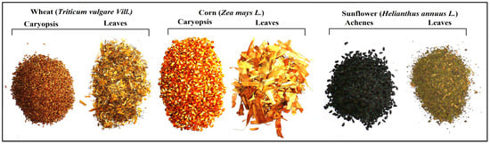
Figure 3.
Samples of crop grains/seeds and leaves after cleaning and drying.
For various analyses, the soil and plant samples were pelletized using the Specac Ltd. (Orpington, UK) hydraulic press (5 tf were applied for soil samples and 4 tf for plant samples). However, the sunflower seeds, which contain oil, could not be pelletized. Therefore, they were analyzed at the surface and in section.
Several methods were employed to determine the chemical properties of soil and plants [1]. The pH was measured according to [18], and organic matter (OM) and organic carbon (OC) levels were determined using [19]. The CaCO3 content was measured by the volumetric method according to [20], while the other properties (SEBs = Sum of Exchange Bases, HA = Hydrolytic Acidity, and DBS = Degree of Base Saturation) were examined as per [21]. To determine the soil EC (Electrical Conductivity) and TDS (Total Dissolved Salts), [22,23] were used. The soil granulometric fractions were employed according to [24].
Moreover, advanced complementary methods were applied at INPOLDE research center of Dunarea de Jos University of Galati and “Horia Hulubei” National Institute for R&D in Physics and Nuclear Engineering (NIPNE) at Magurele, Romania, to study the soil and plant. The mineralogical and elemental analyses were conducted by Scanning Electron Microscopy combined with Energy-Dispersive X-ray analysis (SEM-EDX) and the Attenuated Total Reflectance-Fourier Transform Infrared technique (ATR-FTIR). The High-Resolution Continuum Source Atomic Absorption Spectrometry (HR-CS AAS) method was employed to determine toxic and potential toxic metals, such as Cd, Co, Cr, Cu, Ni, Pb, Zn, and Mn. The non-destructive Particle-Induced Gamma-ray Emission (PIGE) nuclear technique was useful to identify medium atomic mass and light elements (LEs) like Ca, Ti, Fe, as well as Na, Mg, Al, Si, P, and F.
For the determination of the total contents of HMs in soil and plant, the following protocols were applied: for soil. Soil samples were prepared as described above and oven-dried at 105 °C until a constant mass was achieved, as per [25]. Around 1 g of each sample was treated with modified aqua regia, which is a mixture of 2.5 mL HNO3 (69%), 7.5 mL HCl (37%), and 1 mL HF (48%). A control sample was also prepared using the same reagent mixture. The prepared samples were placed in a Berghof microwave oven and digested as follows: Step 1—180 °C, time 15′, power 90%; Step 2—150 °C, time 15′, power 90%; and Step 3—100 °C, time 10′, power 90%. After cooling to room temperature for about 30 min, the digestate was filtered, transferred to 50 mL volumetric flasks, and diluted with 0.5% HNO3. For plant: Approximately 0.3 g of finely ground and dried plant samples was placed in reaction vessels. Then, 6 mL of HNO3 (69%) was added to the vessels and left overnight under a fume hood. The following day, 3 mL of H2O2 (35%) was added to the teflon vessels. For comparison, a control sample was also prepared using the same reagent mixture. The digestion vessels were placed in the Berghof microwave oven, and a four-step digestion program was used as follows: Step 1—140 °C, time 10′, power 90%; Step 2—180 °C, time 15′, power 90%; Step 3—100 °C, time 15′, power 90%; and Step 4—85 °C, time 5′, power 90%. After cooling at room temperature, the digested samples were transferred to 50 mL volumetric flasks and then diluted with 0.5% HNO3. A ContrAA 700 Analytik Jena spectrometer was used to investigate the concentration of HMs in soil and plants employing both flame and graphite oven methods. The results were expressed in mg kg−1 d.w. (dry weight).
The mineralogical compositions of soil and chemical groups in plant structures were analyzed using the ATR-FTIR method, with assistance from a Bruker Tensor 27 FTIR spectrometer that featured an ATR unit coupled with a diamond crystal. Soil and plant samples, prepared as described, were put as a thin layer onto the ATR device. Background correction was performed, and spectra were recorded as an average of 32 scans per analyzed sample within the range of 4000–400 cm−1 and at a resolution of 4 cm−1. Separation of the overlapping bands found into the complex 1250–850 cm−1 absorption band was obtained by deconvolution using OriginPro 2016 (version 9.3.226) software. Curve fitting was performed by setting the number of component bands found by second derivative analysis and Lorentzian profile.
The Scanning Electron Microscopy (SEM) method was used to analyze soil and plant samples to study their microstructure and surface morphology. The SEM images were captured using an SEM microscope, model FEI QUANTA 200, Thermo Fisher Scientific, Hillsboro, OR, USA. During imaging investigations, the electron beam was accelerated to an accelerating voltage of 20 kV, which was sufficient to obtain a secondary electron signal resulting from the excitation of as many constituent chemical elements as possible. The vacuum pressure was set to 60 Pa (medium vacuum), and the working distance was 10 mm. SEM images were taken at various magnifications, ranging from 250X (overview) to 5000X (structural details).
For the SEM analysis, the samples were mounted on an aluminum support using double-adhesive carbon tape, following the protocol described by [26]. After the samples were dried, finely mortared, and pastilled, they were covered with a thin layer of gold before the microscopic analysis. The surface metallization step was performed using SPI Sputter Coater Module equipment (SPI Supplies, West Chester, PA, USA) at a pressure of 6 mbar and a plasma current intensity of 18 mA, resulting in a metal layer with a thickness of 10 nm.
The SEM micrographs were complemented by the X-ray spectra through a semi-quantitative elemental analysis of the samples using the Energy-Dispersive X-ray Spectroscopy (EDX) method. This required the use of a Si (Li) detector, coupled to the SEM microscope. Four different micro areas were randomly selected and analyzed on a surface with an area of 60 μm2, calculating the average value of the percentage concentration of the elements. EDX spectra were recorded at a magnification of 5000X, and the measurement time was 100 s. To eliminate the matrix effect, the ZAF correction algorithm was applied (correction by atomic number (Z), absorbance (A), and fluorescence (F)), as suggested by [26]. The algorithm converted the apparent concentrations (raw spectral line intensity) into semi-quantitative concentrations.
The PIGE technique used a proton beam with an energy of 3 MeV to irradiate environmental samples in a multi-target reaction chamber under vacuum (10−5 mbar). An Ortec HPGe Gamma-ray detector (GEM10PA-70) with a relative efficiency of 10% and a resolution of 1.75 keV at 1332 keV (60Co) was used in the experimental setup. The detector was positioned outside the reaction chamber at a 45° angle to the beam path and the target sample. The finely ground, homogenized, and pressed samples of 1 cm diameter and 1 mm thickness were fixed on a target holder and introduced into the reaction chamber perpendicular on the beam direction.
Specialized software at the 3 MV Tandetron accelerator of NIPNE was used to configure the operating parameters, such as irradiation time (~1200 s for soil and ~2700 s for plants), proton beam position on the target, its dimension (~2 mm diameter), and current (~5 nA for plant and ~22 nA for soil samples). Proton beam electrical charge on the target was in the range of 13–33 μC. Two measurements were taken for each soil/plant sample.
The data were processed using SRIM-2013 software [27] for stopping power assessment of the proton beam in the sample and comparator standard required in applying matrix correction [28], as well as GammaW software version 2.70 [29], for PIGE spectra analysis (elemental characteristic peak areas determination as number of electrical counts). The results obtained through the PIGE method were quantified by establishing a ratio between the elemental concentration in sample and comparator standard/reference material [30]. To determine the elements Na, Cl, Mg, F, Fe, P, Si, and Al, high-purity chemical compounds (NaCl, MgO, CaF2, and Fe2P), as well as Si (monocrystalline) and Al foil, were used as comparator standards. Certified reference materials of a similar matrix to the analyzed material, namely INCT-TL-1 (tea leaves) and INCT-OBTL-5 (Oriental Basma tobacco leaves) for plants, as well as IAEA-356 and IAEA SD-M-2/TM (marine sediment) for soils, were considered for an analytical quality control.
2.4. Pollution and Health Risk Assessment
2.4.1. Pollution Indices
In recent decades, pollution indices have become increasingly valuable in evaluating the degree of soil and sediment contamination [31,32,33,34,35]. These indices provide crucial information about the origin of the contamination, whether it is natural, anthropogenic, or a combination of both. Additionally, they offer insights into the associated risks posed to the environment and human health.
Different pollution indices have been used to evaluate the extent of soil contamination by toxic elements. These include the Geoaccumulation Index (Igeo), Enrichment Factor (EF), Single Pollution Index (PI), the Potential Ecological Risk Index (PERI), the Contamination Severity Index (CSI), and the mean Effect Range Median quotient (mERMQ). These indices provide varying perspectives on the nature and degree of contamination, offering a comprehensive understanding of the contamination state of soil in the given area. The data generated can be useful in making decisions on land use and remediation efforts. The indices were calculated and evaluated according to [36,37,38,39,40].
The Geoaccumulation Index (Igeo), first introduced by [41], is the ratio of the concentration of HMs in soil to their natural geochemical background (Equation (1)).
where Ci refers to the concentration of a particular i metal in the soil (mg kg−1), and Bi refers to the concentration of that same metal in the natural background (mg kg−1). The constant 1.5 is used to facilitate accurate and consistent data analysis, while also minimizing the impact of lithological variations on the overall results. Soil contamination degree was classified according to the scale of interpretation developed by Müller G. as follows: Igeo ≤ 0—unpolluted (Class 0); 0 < Igeo ≤ 1—unpolluted to moderate polluted (Class 1); 1 < Igeo ≤ 2—moderate polluted (Class 2); 2 < Igeo ≤ 3—moderate to high polluted (Class 3); 3 < Igeo ≤ 4—high polluted (Class 4); 4 < Igeo ≤ 5—high to very high polluted (Class 5); and > 5—excessively polluted (Class 6).
The Enrichment Factor (EF), first calculated by [42], is an index that helps to assess the impact of human activities on the concentration of metals in soil. It is calculated by dividing the concentration of a particular metal in the soil by the concentration of a naturally occurring element such as Fe, Al, Sc, Mn, or Zr, which remains constant over time. In this study, the element Al was used as a reference to normalize the metal enrichment (Equation (2)).
where Ci refers to the concentration of the metal i in soil (mg kg−1), CAl is the concentration of aluminum in soil, Bi is the concentration of that same metal in the natural background (mg kg−1), and BAl is the concentration of Al in the natural background. The results were classified by [38] classes of interpretation: Class 1: <2—deficiency—minimal enrichment (unpolluted soil—low polluted soil); Class 2: 2–5—moderate enrichment (moderately polluted soil); Class 3: 5–20—significant enrichment (significant polluted soil); Class 4: 20–40—high enrichment (highly polluted soil); and Class 5: >40—extremely high enrichment (extremely polluted soil).
The Single Pollution Index (PI) is used to identify the metal with the highest impact on environment, and it was calculated according to Equation (3) [39].
where Ci refers to the concentration of the metal i in soil, and Bi is the concentration of that same metal in the natural background, both expressed in mg kg−1. Soil contamination was classified as follows: PIi < 1—uncontaminated (Class 1); 1 < PIi < 2—low contaminated (Class 2); 2 < PIi <3—moderate contaminated (Class 3); 3 < PIi < 5—high contaminated (Class 4); and PIi > 5—very high contaminated (Class 5) [40].
The Potential Ecological Risk Index (PERI), introduced by [43], expresses the probability of the occurrence of an ecological risk due to contamination with toxic or potentially toxic elements. This index was calculated with formula (Equation (4)) [43], and its values are classified after the following scale of interpretation: low potential ecological risk (PERI < 150), moderate potential ecological risk (150 ≤ PERI ˂ 300), high potential ecological risk (300 ≤ PERI ˂ 600), and very high potential ecological risk (PERI ≥ 600) [43].
where n is the number of elements, and Eri is the potential ecological risk of the metal i, which is calculated with Equation (5).
where Tri is the toxic response caused by the exposure of metal i. According to [43], Tri values (mg kg−1) are as follows: TrCd—30, TrCu—5, TrPb—5, TrCr—2, TrZn—2, and TrNi—5. According to [9,40], the ecological risk can be classified as follows: low ecological risk (Eri < 40), medium ecological risk (40 < Eri < 80), considerable ecological risk (80 < Eri < 160), high ecological risk (160 < Eri < 320), and very high ecological risk (Eri > 320).
The Contamination Severity Index (CSI), developed by [44] to assess the degree of soil pollution with HMs, was calculated using the formula provided by [40,45] (Equation (6)).
where Wt is the calculated weight of the metal, Ci refers to the concentration of the metal i in soil, ERLi represents the value at which the impact on living organisms of the metal is low, while ERMi is the value at which the impact on living organisms of the metal is medium. Table 2 displays the HM weight values, as well as ERMi and ERLi values.
Table 2.
Heavy metal weight, ERMi, and ERLi values.
The classification of soil contamination into contamination classes, as per the CSI, is based on the contamination intensity classes defined by [40]. These classes serve as an indicator of the severity of soil pollution present within a given area. The classes are defined as follows: Class 1 (<0.5)—uncontaminated soil; Class 2 (0.5–1.0)—very low level of soil contamination; Class 3 (1.0–1.5)—low level of soil contamination; Class 4 (1.5–2.0)—low to moderate level of soil contamination; Class 5 (2.0–2.5)—moderate level of soil contamination; Class 6 (2.5–3.0)—moderate to strong level of soil contamination; Class 7 (3.0–4.0)—high level of soil contamination; Class 8 (4.0–5.0)—very high level of soil contamination; and Class 9 (>5.0)—excessive level of pollution.
The mean Effect Range Median quotient (mERMQ) was calculated according to [45] as Equation (7).
where Ci refers to the concentration of metal i in soil, ERMi is the value at which the impact on living organisms of the metal is medium, and n is the number of elements. mERMQ is classified into four grades: ≤0.1—low risk, probability of toxicity is 9%; 0.1–0.5—medium risk, probability of toxicity is 21%; 0.5–1.5—high risk, probability of toxicity is 49%; and >1.5—very high risk, probability of toxicity is 76% [45].
2.4.2. Plant Bioaccumulation of Major and Trace Elements
To assess the environmental risk of chemicals, the bioaccumulation factor (BFi) of major and trace elements was calculated according to Equation (8), as it helps to determine the potential for the toxic or potential toxic elements to accumulate in the food chain and ultimately affect human and animal health.
where Ci plant refers to the concentration of element i in plant section (leaf and grain), and Ci soil is the same element content in the soil. A BFi > 1 indicates that the plant has a higher potential to accumulate the element (the plant is called “accumulator”), while 1 < BFi suggests that the plant is less likely to accumulate the element (the plant is called “excluder”), and when BFi = 1, it indicates the soil metal contents (the plant is called “indicator”) [47,48].
Human health risk assessment is a very important process that involves assessing the potential impact of a hazard on the health of people and even the communities they belong to. Due to agricultural practices that cause environmental damage (especially the irrational use of chemical fertilizers, pesticides, amendments, mismanagement of agricultural land use, and the lack of tree planting to optimize soil protection against water and wind erosion, by which a large amount of dust full of toxicants is released into the air and body of water) and industrial activities, which release polluting particles into the atmosphere, in the Lower Danube Basin, heavy metal and other contaminant exposure is an actual concern. The dust dispersed from the surface of the agricultural soils in the vicinity of the TUL (GL), SEN (GL), and VAD (BR) villages is thus inhaled, swallowed, or even deposited on the surface of the skin, generating health risks for the inhabitants, children being the most exposed. For the study area, there is less information about soil and crop contamination with toxic or potentially toxic elements, and less is known about the non-carcinogenic and carcinogenic risks to which the population of adults and children is exposed during their lifetime.
To assess the potential health risk of contaminants, the analytical data for soil elemental composition (Csoil) and also the reference values and equations given by [49,50] and [51] were used (see Equations (9)–(11)).
The chronic daily intake (CDI) for toxic element exposure is estimated by the CDI for ingestion (CDIingestion), dermal contact (CDIdermal), and inhalation (CDIinhalation). The equations employed in this regard are as follows:
where the parameters of non-carcinogenic and carcinogenic health risks and their reference values are presented in Table 3.
Table 3.
Exposure parameters used to assess non-carcinogenic and carcinogenic health risks.
The hazard quotient (HQi) provides information on the non-carcinogenic risk of element i through chronic daily intake of toxic elements (CDI) relative to the chronic reference dose of element i (RfDi, mg kg−1 day−1)—Equation (12).
The RfDi reference values were considered according to [52] as follows: RfDingestion—Cd (1.00 × 10⁻³), Cr (3.00 × 10⁻³), Ni (2.00 × 10⁻²), Co (3.00 × 10⁻⁴), Cu (4.00 × 10⁻²), Pb (3.50 × 10⁻³), and Zn (3.00 × 10⁻¹); RfDdermal—Cd (1.00 × 10⁻⁵), Cr (6.00 × 10⁻⁵), Ni (5.40 × 10⁻³), Co (1.60 × 10⁻²), Cu (1.20 × 10⁻²), Pb (5.25 × 10⁻⁴), and Zn (6.00 × 10⁻²); and RfDinhalation—Cd (1.00 × 10⁻³), Cr (2.86 × 10⁻⁵), Ni (2.06 × 10⁻²), Co (5.71 × 10⁻⁶), Cu (4.02 × 10⁻²), Pb (3.52 × 10⁻³), and Zn (3.00 × 10⁻¹).
When the hazard quotient (HQ) is greater than 1, it indicates that the exposed individuals are likely to experience adverse health effects. Conversely, when the HQ is less than 1, it suggests that there is no health risk for the exposed individuals [51].
The potential non-carcinogenic risk effects that may occur were investigated by hazard index (HI) using Equation (13).
When the HI is greater than 1, it indicates a higher likelihood of a toxicological response to the exposure of harmful substances through multiple pathways. Conversely, an HI score below 1 suggests a low probability of a toxicological response to the combined harmful exposure [51,53].
3. Results and Discussion
3.1. Assessment of Soil Main Parameters That Influence the Elemental Bioavailability
The soil’s natural exchanges with the plants it supports are influenced by the following soil parameters: pH, CaCO3 content, SEB, HA, DBS, OM, OC, TDS, and soil texture. Soil main properties of the investigated soils are presented in Figure 4. The role of soil parameters in retaining and releasing nutrients and harmful elements is widely recognized. Humus, a vital component for soil fertility, enhances soil structure and water retention, directly impacting the availability of nutrients [54]. The soil’s pH plays a crucial role in plant development, influencing nutrient uptake and the movement of both toxic and non-toxic metal ions [55,56,57]. Even at low concentrations, dissolved salts can hinder plant growth and nutrient absorption. Furthermore, the distribution of sand, silt, and clay in the soil affects the absorption and availability of major and minor chemical elements. Each soil texture type possesses unique water retention and nutrient-holding capacities [58,59].
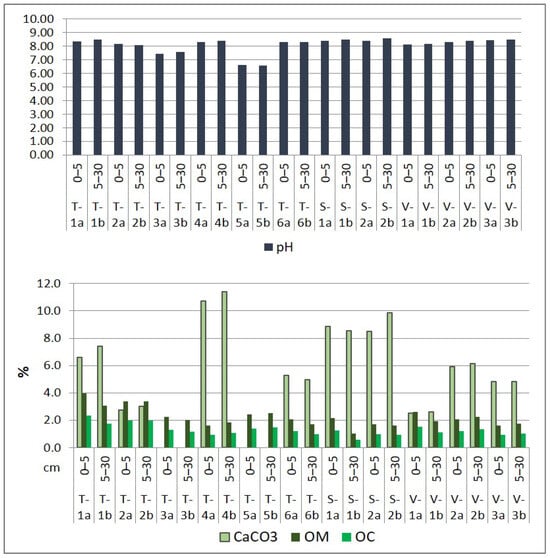
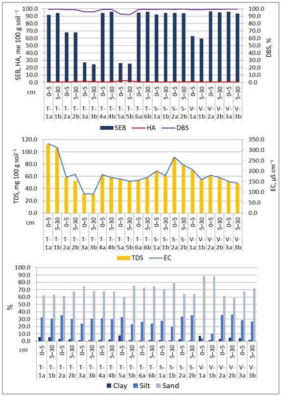
Figure 4.
Physico-chemical properties of surface soil in the Lower Danube Basin (Tulucesti, Sendreni, and Vadeni areas) (after [1,60]).
The soil’s pH showed a similar distribution on both layers and on the three assessed territories. Generally, the pH is slightly alkaline, ranging between 7.44 and 8.44 on the first layer (0–5 cm) and 7.59 and 8.48 on the second layer (5–30 cm). However, site T-5a/5b is an exception, where the pH is slightly acidic, measuring 6.63 on the first soil section and 6.56 on the second soil section. The CaCO3 level in the first 30 cm of soil layer varies from medium to high, ranging between 2.52% and 11.42. In sites T-3a/3b and T-5a/5b, where the pH is the lowest, CaCO3 is absent. The levels of OM and OC are impacted by the distribution of granulometric fraction. The OM levels vary from low to high, ranging between 1.61% and 3.98% in the first soil section and between 1.00% and 3.37% in the second soil section. The SEB values recorded from 68.18 to 96.51 me 100 g soil−1 in the 0–5 cm layer and 59.65 to 95.34 me 100 g soil−1 in the 5–30 cm layer. Meanwhile, HA levels were very low, with measurements ranging between 0.43 and 1.22 me 100 g soil−1 in the 0–5 cm layer and 0.38 and 1.09 me 100 g soil−1 in the 5–30 cm layer. The only exception was the T-5b site, where the AH value was 2.22 me 100 g soil−1. Overall, the soil showed a high Degree of Base Saturation, with DBS values ranging from 99.03% to 99.52% in the first 5 cm layer and from 91.99% to 99.60% in the 5–30 cm layer. Additionally, we evaluated the EC and TDS, which indicated that the soils were generally unsalinized, with the exception of soil samples from the T-1a/1b site located in the Prut meadow, which overlaps alluvial deposits (Figure 4).
The soil is classified predominantly as coarse due to the high percentage of sand in comparison with clay and silt. The soil texture distribution is as follows: medium sandy loam (T-1a, T-1b), fine sandy loam (T-5a), fine sand (T-2a, T-2b, T-3a, T-3b, T-4a, T-4b, T-5b, S-1a, S-1b, V-3a, V-3b), medium sand (T-6a, T-6b, V-a, V-1b), and sandy silt (S-2a, S-2b, V-2a, V-2b). These textural classes were also identified by [61] for this region.
3.2. Major and Trace Element Assessment in Soil
Soil levels of contamination in the top layer’s sections, expressed in mg kg−1 dry weight (d.w.), are illustrated in Figure 5, together with the normal value (NV), alert threshold (AT), and intervention threshold (IT) specified by Romanian legislation (Table 4).
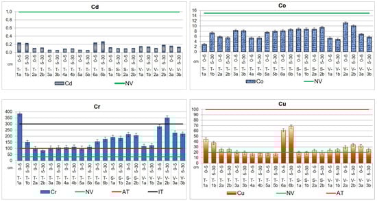
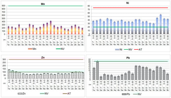
Figure 5.
Heavy metal distribution in the upper layer, up to 30 cm, of agricultural soils from the Lower Danube Basin (T—Tulucesti, S—Sendreni, and V—Vadeni) determined by the HR-CS AAS technique (in mg kg−1 d.w.).
Table 4.
Average concentration values of trace (mg kg−1 d.w.) and major (in% d.w.) elements in the upper layer of continental crust, world, European, and Romanian soils synthesized after various authors and the Ministry of Water, Forests, and Environmental Protection of Romania [62,63,64,65,66,67,68].
The results were compared with the average values of major and trace element content presented in Table 4, synthesized after [62,63,64,65,66,67,68].
3.2.1. Heavy Metals in Soil
The average concentrations of Cd, Co, Mn, and Pb in agricultural soils did not go beyond Romanian standards [67] and are lower than the levels presented in Table 4. The results showed a pronounced impact of the steel industry (mainly in the downwind direction) and agricultural activities on the content of Cr, Cu, Ni, and Zn in the soil.
In the three targeted ATUs, chromium exhibits the NV, and AT is even higher than the IT in several locations. Thus, the highest values were obtained for T-1a and V-2b, evidencing a high contamination. Most samples registered concentrations beyond the AT, and their Cr values ranged as follows: 102.0–175.5 mg kg−1 (TUL), 183.5–215.4 mg kg−1 (SEN), and 117.1–277.4 mg kg−1 (VAD).
For nickel, it can be noticed that all the investigated sites of the three ATUs are contaminated. The findings of our study reveal higher levels of Ni than NV, the concentrations,50,300…… being similar for TUL (39.6 mg kg−1 for the first soil section and 38.8 mg kg−1 for the second soil section) and SEN (39.1 mg kg−1 for the first soil section and 37.0 mg kg−1 for the second soil section) territories. In the case of VAD area, the values are higher (40.4 mg kg−1 for the first section and 42.8 mg kg−1 for the second one) than in SEN and TUL sites.
The results obtained for copper indicate that levels exceed the NV in certain locations in TUL and SEN territories (T-1a,b, T-2a,b, T-3a, T-6a,b (TUL), S-2a (SEN)), while in VAD territory, they exhibit NVs in all the sampling sites. The Cu mean values are between 17.1 and 17.8 mg kg−1 in TUL and between 18.9 and 19.8 mg kg−1 in SEN in the non-polluted sites. In the sites where the content exhibits the NV, the values are ranging from 20.7 to 68.1 mg kg−1 (TUL) and 22.9 mg kg−1 (SEN). In VAD territory, where all the values are beyond the NV, Cu content ranges between 23.3 and 34.1 mg kg−1.
The Zn load in agricultural soil is in order VAD > TUL > SEN, having the following mean levels: 89.1 mg kg−1 (VAD), 87.0 mg kg−1 (TUL), and 74.4 mg kg−1 (SEN) for the first soil section; 89.0 mg kg−1 (VAD), 82.6 mg kg−1 (TUL), and 67.3 mg kg−1 (SEN) for the second soil section. The maximum concentration values for Zn in soil were found in TUL area (T-1a,b and T-2a) and in VAD area (V-2b and V-3a).
3.2.2. Other Major and Trace Elements in Soil
In conducting soil analysis within the Lower Danube Basin, PIGE nuclear method proved particularly useful in identifying and quantifying LEs, including Al, Mg, Na, Cl, Si, and F. Some of these elements, such as fluorine, can be hazardous even in low amounts. Figure 6 illustrates the distribution of light elements in the upper layer of the agricultural soil in the Lower Danube Basin.
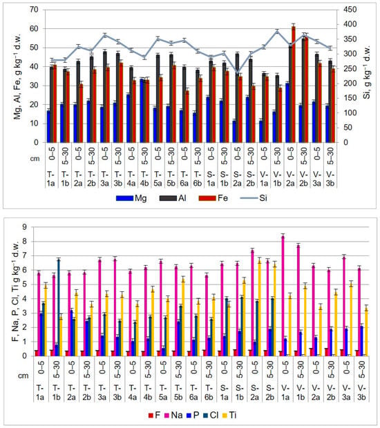
Figure 6.
Light element distribution and concentration in upper layers of agricultural soils in the Lower Danube Basin, determined by PIGE technique (g kg−1 d.w.).
In the TUL region, sodium levels in the 0–5 cm layer range from 5.8 to 6.7 g kg−1, while in the 5–30 cm layer, they vary from 5.6 to 6.7 g kg−1. Aluminum content ranges between 39.7 and 47.8 g kg−1 (0–5 cm) and 32.8 and 46.3 g kg−1 (5–30 cm). Silicon concentration in the first soil section is between 278.5 and 363.8 g kg−1, while in the second soil section, it ranges from 279.1 to 341.3 g kg−1. Chlorine shows the lowest content values compared to other elements. In the first 5 cm layer, it falls within the range of <2.4–<3.7 g kg−1, while in the second layer, it varies between <0.2 and <6.7 g kg−1.
In the SEN area, the uppermost soil layer (0–5 cm) has a sodium content ranging from 6.4 to 7.3 g kg−1. In the second soil section, sodium values range between 6.4 and 6.6 g kg−1. The aluminum level ranges from 43.0 to 46.6 g kg−1 (0–5 cm) and from 41.9 to 43.9 g kg−1 (5–30 cm). Silicon content follows a similar trend, with concentrations ranging from 234.8 to 288.5 g kg−1 in the first 5 cm of soil and from 300.4 to 302.2 g kg−1 in the next 25 cm. Chlorine, on the other hand, has low concentrations that fall below <3.8–<4.0 g kg−1 at 0–5 cm and <4.0 <4.1 g kg−1 at 5–30 cm.
In the VAD land, the sodium content ranges from 6.3 to 8.3 g kg−1 in the top 5 cm of soil, while in the next 25 cm layer, it is between 6.0 and 7.7 g kg−1. In the first soil section, aluminum concentrations range from 36.3 to 51.0 g kg−1, and in the second soil section, they range from 35.3 to 54.7 g kg−1. The silicon content in the top 5 cm of soil is comparable to that of agricultural soil found in the TUL and SEN regions. The values range from 324.1 to 342.2 g kg−1. In the second soil section, the silicon content ranges from 319.1 to 375.9 g kg−1.
The analysis of agricultural soils has shown a variable accumulation of Fe between soil layers and territorial distribution. In TUL, higher concentrations of Fe were observed at the depth of 5–30 cm, with values ranging from 32.9 to 41.9 g kg−1 compared to the first layer, where the values vary between 27.2 g kg−1 and 39.5 g kg−1. However, soil sampled from site T-1 shows higher values in the 0–5 cm layer (40.719 ± 4.316 g kg−1 d.w.) compared to the underlying 5–30 cm layer (37.289 ± 7.048 g kg−1 d.w.). In SEN and VAD, higher concentrations of Fe were found in the upper 0–5 cm layer, with values ranging from 34.7 g kg−1 to 39.4 g kg−1 and from 34.5 g kg−1 to 61.0 g kg−1, respectively. In the 5–30 cm layer, the concentrations vary between 29.5 g kg−1 and 37.4 g kg−1 in SEN and between 28.7 and 38.8 g kg−1 in VAD. According to [62], the average value of Fe in soil is 35 g kg−1. The highest value of Fe concentration was recorded at sampling site V-2, at both depths, with values of 61.0 g kg−1 and 55.8 g kg−1, respectively.
Titanium values are lower than the average concentration in soil presented in Table 4. In TUL, the values range between 3.6 g kg−1 and 4.9 g kg−1 in the first soil section and from 2.7 g kg−1 to 5.3 g kg−1 in the second soil section. In SEN, the concentration of Ti in the first layer ranges between 3.6 g kg−1 and 6.6 g kg−1, and in the second layer, the values are from 5.2 g kg−1 to 6.4 g kg−1. In VAD, the values vary between 3.4 g kg−1 and 5.0 g kg−1 in the first soil section and between 3.3 g kg−1 and 4.9 g kg−1 in the second soil section.
Through PIGE technique, it was possible to identify fluorine, an extremely harmful element that negatively impacts ecosystems. Fluorine is typically associated with bone disease [69] and can disrupt the processes of photosynthesis and respiration in plants [70]. In most living organisms, the concentration of fluoride is less than 10 µg g−1 d.w. [71]. According to [62], soils worldwide have an average fluoride content of 321 mg kg−1, while the continental crust has a value of 625 mg kg−1. In the analyzed soils, fluoride exceeds the global average and the Romanian norms. For instance, in TUL and SEN, fluoride content values range from 0.3 g kg−1 to 0.4 g kg−1 in both considered soil sections. The fluoride concentration in the soil from VAD territory is 0.3–0.5 g kg−1, in both soil layers. Notably, sampling point V-2, located on the right side of the European road E87 in the Sendreni-Baldovinesti segment, has slightly higher fluoride concentrations at both depths compared to other sampling points on the territory of Vadeni. The main sources of soil contamination with fluoride are emissions from metallurgical activities and the use of phosphate fertilizers and pesticides [72].
3.3. Mineralogical and Microstructural Analyses of Soil
Soils encompass a complex array of chemical components, comprising both mineral factions such as clays, oxides, and quartz as well as organic fractions constituted by organic matter in various stages of decomposition. Additionally, soils contain water and air. The intricate composition of soils renders them a challenging material to study, requiring a comprehensive approach that considers the interplay of the various components.
Based on the soil ATR-FTIR spectra featured in Figure 7, it is evident that the absorption bands of the analyzed soil samples share similarities, but their peak intensities differ. This indicates the presence of various functional groups of chemical elements, which are characteristic of both clay minerals and non-clay minerals.
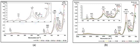
Figure 7.
Soil ATR-FTIR spectra in the 4000–400 cm−1 region and 1800–400 cm−1: (a) the first soil section; (b) the second soil section.
Within the spectral range of 1500–400 cm−1, known as the “spectral fingerprint domain” [73], distinctive absorption bands of clay minerals including montmorillonite ((Na,Ca)0.33(Al,Mg)2(Si4O10)(OH)2·nH2O) and kaolinite (Al2Si2O5(OH)4) were identified. Additionally, non-clay minerals such as quartz (SiO2), feldspars (orthose (KAlSi3O8), albite (NaAlSi3O8)), and calcite (CaCO3) were also recognized. Table 5 displays the ATR-FTIR peaks that represent the functional groups associated with the primary minerals present in the studied soils. To emphasize the absorption bands in the 850–1250 cm−1 range, the ATR-FTIR spectra were deconvoluted, as illustrated in Figure 8 [74].
Table 5.
Characteristic absorption bands associated with the vibrations of the functional groups of the main minerals found in the selected soil samples [1].
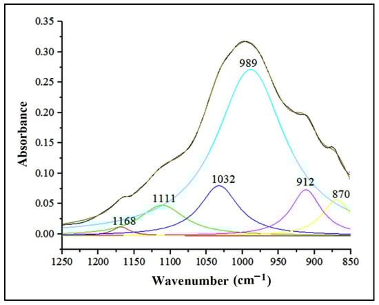
Figure 8.
Deconvolution of the IR absorption bands in the range 1250–850 cm−1.
The selected soil samples were found to contain montmorillonite and kaolinite minerals from the category of clay minerals. The stretching vibrations of the hydroxyl functional group (-OH) were attributed to these domains within the limits of 3390–3620 cm−1 and 3620–3695 cm−1, respectively. Reference [80] mentioned that the values of wave numbers in the range 3610–3621 cm−1 are characteristic of abnormal montmorillonite, a category of mineral widespread in most soils, which presents a single dehydroxylation reaction, while [76] reported that in the case of abnormal montmorillonite, the stretching vibration of the -OH group is highlighted by the peak with the value 3625 cm−1.
In the case of kaolinite, the asymmetric stretching vibration of the Si-O-Si group in the 1032 cm−1 area was noticeable. The bending vibrations attributed to functional groups Al-OH-Al (912 cm−1), Al-OH-Mg (830 cm−1), and Si-O-Si (419 cm−1) were recorded in the 1000–400 cm−1 area from the structure of clay minerals.
The peaks at 778 cm−1, 796 cm−1, 1001 cm−1, 1111 cm−1, and 1168 cm−1 are attributed to the symmetric and asymmetric stretching vibrations of the Si-O and Si-O-Si groups in the quartz structure. The highest absorbance was recorded for the peak at wave number 1001 cm−1. Reference [75] assigned the bands in the range 1115–1105 cm−1 (1001 cm−1 and 1111 cm−1 for the selected soils) to the asymmetric stretching vibration of the Si-O-Si group in amorphous silica. At the same time, the deformation vibrations of the Si-O-Si group, fully registered in the range 692–457 cm−1, are noted. Reference [76] assigned the 1166 cm−1 peak to cristobalite, a variety of quartz with a tetragonal crystal structure, and [75] reported that wave number 778 cm−1 corresponds to α-quartz, variety with the trigonal crystalline structure.
A particular situation is given by the absorption band of 1111 cm−1, highlighted in the deconvolution zone of the complex of bands in the range 1250–850 cm−1 (Figure 8), which, according to [76], is associated with gypsum (CaSO4∙2 H2O). The vibrational mode of the SO42- ion in the 1111 cm−1 band corresponds to the deformation vibration associated with the 646 cm−1 peak, reduced in intensity. Close values for sulfate vibrational modes are reported by [75] and [81].
The absorption band at 989 cm−1, which is attributed to the Si-O group’s stretching vibration, confirmed the presence of feldspars in the assessed soils. This absorption is highlighted by a pronounced peak in the deconvolution zone (Figure 8). Additionally, a secondary absorption band at 646 cm−1 was attributed to the O-Si(Al)-O group’s deformation vibration, marked by a peak with low intensity (Figure 7). As stated by [78], calcite is characterized by two intense bands—1400 cm−1, attributed to the asymmetric stretching vibration, and 875 cm−1, specific to the out-of-plane deformation vibration. The selected soil samples’ absorption band values are around those replicated in the literature (Table 5). The values include a more intense absorption band, centered around 1433 cm−1, attributed to the C-O group’s asymmetric stretching vibration, and two narrower bands centered at 874 cm−1 and 712 cm−1, characteristic of the same group’s deformation vibration.
The ATR-FTIR spectra of the studied soil samples also highlight the presence of dolomite through the maximum peak centered at 1433 cm−1, attributed to the asymmetric stretching vibration of the CO32− ion [82], present in the chemical composition of this mineral (Ca Mg(CO3)2).
The intensity of the peaks associated with the characteristic absorption bands of calcite at 1433 cm−1 and 874 cm−1 (Figure 7) is directly proportional to the percentage of CaCO3 in the soil.
The very low organic carbon percentages correlate with the absence of peaks in the ATR-FTIR spectrum. Specifically, the peaks at 2920–2926 cm−1 and 2850–2852 cm−1, which are indicative of the symmetric and antisymmetric stretching vibrations of the functional group CH2 [79,81], are absent. The ATR-FTIR spectra of the soils examined in this study closely resemble those obtained by [83] for soils collected from parks located in the city of Galați, confirming the mineralogical footprint of the region.
The SEM-EDX technique was very valuable for examining the mineralogy of the soil and providing a semi-quantitative analysis of its elemental composition (Figure A1, Appendix A). Additionally, the results from SEM-EDX mapping (Figure A1, Appendix A) confirmed the findings obtained through the ATR-FTIR method. The analysis indicates a consistent elemental composition across the studied soils in the Lower Danube Basin.
The SEM-EDX semi-quantitative results (Appendix A, Table A1) revealed the distribution of major and trace element content in agricultural soils, as shown in Figure 9.
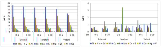
Figure 9.
Elemental distribution in top 30 cm of agricultural soils from the Lower Danube Basin, determined by the SEM-EDX method.
The concentrations of O and Si were the highest among the 24 identified elements. (Appendix A, Table A1). Notably, the O level in soil is lower compared to the value of this element in Earth’s crust (46%) [84].
Silicon, a trace element present in plants and soils, exhibits variable concentrations across different soils and plant species. It constitutes 65.4% (SiO2) of the upper layer of European soils [63] and accounts for 27% of the Earth’s crust [84]. Silicon plays a crucial role in promoting plant growth and influencing the availability and accumulation of both macro- and micronutrients [85]. In soil, silicon exists in both liquid and solid states, with the solid form being either amorphous (derived from the parent rock or living organisms) or crystalline (present in primary and secondary silicates and silicate materials) [86]. The presence of silicon in soil samples is validated using the ATR-FTIR method, which identifies the absorption bands characteristic of the chemical bonds formed by silicon with other elements in the soil’s clay and non-clay minerals.
In the analyzed samples, varying concentrations of alkaline elements (sodium, magnesium, potassium, and calcium) were found (Appendix A, Table A1). The alkaline metals content in the Earth’s crust is in the following order: Ca (5.0%) > Mg (2.9%) > Na (2.3%) > K (1.5%) [84].
3.4. Assessment of Soil Contamination
The evaluation of soil contamination levels involved the use of pollution indices that facilitate comparisons between the degree of assessed soil contamination and the natural background incidence of identified metals.
The Igeo was estimated using the normal values specified in Romanian Order no. 756/1997 [60] (Table 4) as the geochemical background [1]. The results obtained for Igeo are presented in Table 6.
Table 6.
Igeo index values calculated for the agricultural layers of soil in the Lower Danube Basin.
According to the values obtained for Igeo, all the soil samples were considered to be in Class 0—unpolluted with Cd, Co, Pb, Zn, and Cu (except sampling sites T-1a, T-1b, V-3a); in Class 1—unpolluted to moderate pollution with Ni (all the samples), Cr (sites T-2b), and Cu (sites T-1a, T-1b, V-2b, V-3a); Class 2—moderate polluted with Cr (sites T-1a, S-1a, S-1b, S-2a, S-2b, V-2a, V-2b); and Class 3—moderate to high polluted with Cr (sites T-1a, S-1a, S-1b, S-2a, S-2b, V-2a, V-2b, V-3a, V-3b).
To evaluate the impact of anthropogenic activities, the Enrichment Factor (EFi) was computed utilizing aluminum (Al) as a normalizer element, which is found in abundant quantities in the geological background [1]. Considering the values for Al in European topsoil [63], EF indicates Cd, Co, Pb (except site T-1b), Zn (sites T-3a, T-3b, T-5a, T-5b, T-6a, T-6b, S-1a, S-1b, S-2a, S-2b), deficiency to minimal enrichment (Class 1); Cu (except sites T-1b, T-6b), Ni (sites T-1a, T-1b, T-2b, T-5b, T-6a, T-6b, S-1b, V-1a, V-2a, V-2b, V-3a, V-3b), Zn (sites T-1a, T-1b, T-2a, T-2b, T-4a, T-4b, V-1a, V-1b, V-2a, V-2b, V-3a) moderate enrichment (Class 2); Cr (except site T-1a, V-2a, V-2b, V-3a, V-3b), Cu (sites T-1a, T-6b), Ni (sites T-2a, T-3a, T-3b, T-4a, T-4b, T-5a, S-1b, V-1a, V-2a, V-2b) significant enrichment (Class 3); and Cr (site T-1a, V-2a, V-2b) high enrichment (Class 4). Based on EFi quantification, Table 7 displays the distribution of soil metal enrichment due to human activity.
Table 7.
EFi index quantification for the agricultural layers of soil in the Lower Danube Basin.
Upon analyzing the EF values derived from the concentration of Cr, Cu, Ni, and Zn found in the uppermost layers of agricultural soils, it becomes apparent that the origins of these elements are multifaceted, encompassing both past and present factors. The extended duration of land cultivation and the industrial practices of the adjacent iron and steel plant are the primary contributors.
According to PIi values (Table 8), soil is uncontaminated (Class 1) with Cd, Co, Cu (sites T-3b, T-4a, T-4b, T-5a, T-5b, S-1a, S-1b, S-2b), Pb, and Zn (sites T-2b, T-3a, T-3b, T-4a, T-4b, T-5a, T-5b, T-6a, T-6b, S-1a, S-1b, S-2a, S-2b, V-1a, V-1b, V-2a, V-3b), low contaminated (Class 2) with Cu (sites T-1b, T-2a, T-2b, T-3a, S-2a, V-1a, V-1b, V-2a, V-2b, V-3a, V-3b), Ni (T-1a, T-1b, T-2b, T-4a, T-4b, T-5b, T-6a, T-6b, S-2a, S-2b, V-1a) and Zn (sites T-1a, T-1b, T-2a, V-2b, V-3a), moderately contaminated (Class 3) with Cr (site T-2b), Cu (site T-1a), and Ni (sites T-2a, T-3a, T-3b, T-5a, S-1a, S-1b, V-2a, V-2b, V-3a, V-3b), highly contaminated (Class 4) with Cr (sites T-1b, T-2a, T-3a, T-3b, T-4a, T-4b, T-5a, T-5b, V-1a, V-1b) and Cu (sites T-6a, T-6b), and very highly contaminated (Class 5) with Cr (sites T-1a, T-6a, T-6b, S-1a, S-1b, S-2a, S-2b, V-2a, V-2b).
Table 8.
PIi values for the agricultural layers of soil in the Lower Danube Basin.
All soil samples from TUL, SEN, and VAD areas have a low risk of soil enrichment based on PERI evaluation. (Table 9).
Table 9.
PERI and Eri values for the agricultural layers of soil in the Lower Danube Basin.
The Contamination Severity Index (CSI) was used to evaluate the level of toxicity in the soil environment and identify any adverse impacts. The results for CSI (Table 10) indicated that, overall, there was a very low level of soil contamination (Class 2). However, in specific sites such as T-1a, T-1b, S-1a, S-1b, and V-1a, the CSI values highlighted a low level of soil contamination (Third Class).
Table 10.
Soil level of contamination according to CSI and mERMQ indices.
The mERMQ index was utilized to assess the potential for metal toxicity in the soil environment. The results for mERMQ (Table 10) show a relatively low risk with a probability of toxicity estimated at 9%. These findings reveal that the potential for metal toxicity in the soil ecosystem is not a significant cause for concern.
3.5. Major and Trace Element Assessment in Crops
The study of toxic element contamination in crop plants is crucial for understanding the transfer of pollutants through the soil–plant system in agricultural areas located near industrial platforms. Knowing the concentrations of chemical elements in plants intended for human and animal consumption can help plan and implement measures to reduce the risk of contamination through the food chain.
Heavy metal (HM) bioavailability and accumulation in plants are determined by the soil characteristics [1]. Parameters such as pH, clay content, CaCO3, and OM concentration influence the ion mobility of chemical elements [62,87]. Moreover, the metal bioaccumulation in plants is contingent upon the stage of vegetation, species, and the ecologic characteristics of the region where the plants thrive. Certain plants exhibit the capacity to accumulate and process hazardous elements, thereby establishing their significance as bioindicators.
In recent years, experiments have been carried out on phytoremediation, which is the process of using plants to remove, degrade, or immobilize environmental contaminants [88,89,90,91]. Sunflower has shown to be a good hyperaccumulator for toxic or potentially toxic elements such as Cr, Ni, Pb, Zn, Cu, and Cd. Under these conditions, crops have to be monitored in terms of nutritional composition and potential elements with health risks, even in smaller quantities.
The analytical results obtained for the level of heavy metals in wheat and corn grains and sunflower seeds (expressed in mg kg−1 dry weight (d.w.)) (Table 11) comply with the maximum values provided in [92], Codex Alimentarius [93], and [94] for certain contaminants in foodstuffs (Table 12). For Co, Cr, Cu, Ni, Pb, and Zn, European regulations do not provide a limit threshold in cereals and oilseeds. Similarly, no limit values are provided for heavy metals in the vegetative organs of cereals and sunflower. If these plants are used in mixtures for animal feed, the concentrations of the mixture should not exceed the maximum permitted values provided in Directive 2002/32/EC [95] on undesirable substances in feed, as amended.
Table 11.
The heavy metal content (in mg kg−1 d.w. ± standard deviation (σ)) in wheat, corn, and sunflower sections collected from agricultural lands in the Lower Danube Basin.
Table 12.
The maximum permissible levels (MPLs) of heavy metals in the grains and seeds of wheat, corn, sunflower, and crops according to different authors.
3.5.1. Heavy Metals in Plants
The concentration of Cd in wheat ranges from 0.001 ± 0.001 to 0.040 ± 0.003 mg kg−1 in the leaves and from 0.000 ± 0.000 to 0.046 ± 0.003 mg kg−1 in the grains. The mean content of Cd in grains falls within the [93,94] recommendations for all sampling sites. Reference [62] reports average values of Cd in wheat grains, grown under various conditions, of 4.5–270.0 mg kg−1. Reference [96] shows that Cd accumulation in plants occurs in the order root > stem > grain when applying Cd treatments in different concentrations to the soil in wheat and corn. The present study confirms the higher accumulation in leaves than in grains (site S-1), but higher concentration in the grains than in the leaves (sites T-1, T-2). Therefore, careful monitoring of this crop is required due to the tendency of transfer of Cd in grains.
In corn, the mean content of Cd is from 0.056 ± 0.002 to 0.093 ± 0.001 mg kg−1 in the leaves and from 0.003 ± 0.001 to 0.012 ± 0.001 mg kg−1 in the grains. These values fall within the maximum permissible limit recommended by [92,93]. Reference [96] shows that Cd accumulates in large quantities in the root and stem at increasingly high concentrations of Cd in the soil, unlike the grain, which makes corn able to be used as a hyperaccumulator in polluted areas, without posing risks to consumers, provided that the contaminated tissues are not used for animal feed.
In sunflower, Cd content ranges in the limits 0.171 ± 0.005–0.361 ± 0.007 mg kg−1 in the leaves and 0.114 ± 0.001–0.400 ± 0.004 mg kg−1 in the seeds. The values do not exhibit the MPLs for Cd, as established by [92] and [93]. Reference [89] shows that sunflower accumulates Cd more in the root, and the concentration of this element in the plant decreases in the order root > stem > leaves. At the same time, the study of [97] on the ability of sunflower to phytoextract Cd shows that it is a good hyperaccumulator of this element, especially at the root level.
In wheat, Co content lies in the range of 0.030 ± 0.002–0.563 ± 0.015 mg kg−1 in the leaves and 0.009 ± 0.001–0.062 ± 0.005 mg kg−1 in the grains. The highest concentration of Co in leaves was found at sampling site S-1, located near the slag dump. In corn, the concentration of Co ranges from 0.038 ± 0.001 to 0.050 ± 0.003 mg kg−1 in the leaves and 0.003 ± 0.001–0.008 ± 0.001 mg kg−1 in the grains. The pattern of cobalt accumulation in sunflowers mirrors that observed in wheat and corn. In this case, Co level ranges from 0.021 ± 0.002 to 0.128 ± 0.011 mg kg−1 in the leaves and from 0.010 ± 0.001 to 0.047 ± 0.004 mg kg−1 in the seeds.
In Europe, no maximum threshold has been established for the concentration of cobalt in cereals and sunflower seeds. The present study shows that Co accumulates in the order of leaf > caryopses/achenes. Other studies have reported the following concentrations of Co in crop plants: 0.14–0.49 mg kg−1 in wheat grains [98,99] and 0.15–0.24 mg kg−1 in corn grains [98,100].
The results on wheat sections found that Cr concentration tends to be higher in the leaves (0.649 ± 0.055 to 2.707 ± 0.093 mg kg−1). In grains, the concentration was from 0.100 ± 0.004 to 0.801 ± 0.050 mg kg−1. The highest concentrations of Cr were found in sampling sites T-2 (TUL), S-1 (SEN), and V-1, (VAD). The results suggest that the concentration of Cr in different parts of the wheat plant is influenced by the ecological conditions in which the plants grow.
In corn, the highest concentrations of Cr were found in the leaves, with concentrations ranging from 2.386 ± 0.0071 to 2.501 ± 0.011 mg kg−1 d.w., while in caryopsis, the concentration ranged from 0.246 ± 0.016 to 0.547 ± 0.052 mg kg−1 d.w. The average value of Cr in leaves and corn grains was 2.077 mg kg−1 and 0.361 mg kg−1, respectively, when cultivated on soils fertilized with sewage sludge [101].
The accumulation of chromium in sunflowers demonstrated a distinct pattern, with the achenes containing the highest concentrations (0.711 ± 0.033–2.095 ± 0.055 mg kg−1), whereas in the leaves, it varies between 0.042 ± 0.002 and 0.714 ± 0.039 mg kg−1. Reference [101] suggests that both corn and sunflower are good accumulators of Cr, particularly in the root. According to his study, the concentration of Cr decreases in the following order: root > stem > leaves > achenes for sunflower and root > leaves > stem > caryopsis for corn. There are no regulated maximum values allowed for total Cr in the edible sections of crops. However, Table 12 presents the permissible limit of Cr in crops reported by [94].
In wheat, the leaves recorded the lowest Cu average values ranging from 5.825 ± 0.115 to 25.968 ± 1.195 mg kg−1, while the average level of Cu in caryopsis ranged from 8.218 ± 0.177 to 58.397 ± 0.467 mg kg−1. This indicates that the concentration of Cu in wheat is higher in the caryopsis than in the leaves.
In corn, the concentration of Cu was found to be higher in the leaves, with an average concentration of 20.539 ± 0.0270–22.779 ± 0.307 mg kg−1 compared to caryopsis, where the values were between 1.268 ± 0.074 and 3.076 ± 0.017 mg kg−1. This demonstrates that the distribution of Cu in corn varies between leaves and caryopsis.
In the case of sunflowers, in TUL area, the mean concentration of Cu in the leaves ranges between 11.859 ± 0.073 and 86.089 ± 0.863 mg kg−1. In seeds, the concentration varies from 28.958 ± 0.230 to 54.319 ± 0.363 mg kg−1, with the maximum value recorded at sampling site I-6. In SEN area, the mean content of Cu is 535.348 ± 0.535 mg kg−1 in the leaves, while in VAD area, it varies between 235.947 ± 6.842 and 318.245 ± 8.911 mg kg−1. In the seeds, Cu content is between 80.496 ± 0.724 and 120.146 ± 8.290 mg kg−1, S-2 registering the maximum concentration. The distribution of Cu in sunflowers varies significantly depending on the location and the agricultural chemical treatments of the plant.
The concentration of Cu in wheat and corn was found to be below the maximum limit recommended by [94] for crops, which is 73.30 mg kg−1. However, in sunflowers, the concentration of Cu exceeded the limit in some cases. The maximum permissible limits of Cu content regulated in Europe for sunflower seeds are not defined. Therefore, the results for sunflowers indicate the need for further research to determine the safe limits of Cu content in sunflower seeds. According to [62], the range 20–100 mg kg−1 can be used to assess the Cu toxicity threshold of plants.
The findings of our study reveal that the concentration of nickel exhibits a higher presence in the wheat leaves in comparison to the caryopses. The average Ni concentration in the leaves ranges from 0.771 ± 0.047 to 4.130 ± 0.235 mg kg−1, while in the caryopses it ranges from 0.400 ± 0.034 to 1.164 ± 0.115 mg kg−1.
Similarly, for corn, the average Ni concentration is higher in the leaves compared to the caryopses. The average Ni concentration in the leaves ranges from 0.885 ± 0.094 to 1.147 ± 0.001 mg kg−1 d.w. and in the caryopses, it ranges from 0.094 ± 0.065 to 0.718 ± 0.034 mg kg−1 d.w.
On the other hand, in the case of sunflowers, the Ni concentration is higher in the seeds than in the leaves. The mean Ni content in the achenes ranges from 3.797 ± 0.106 to 6.816 ± 0.144 mg kg−1 d.w., while in the leaves, it ranges from 0.511 ± 0.023 to 5.005 ± 0.445 mg kg−1 d.w. It is worth noting that there are no established maximum allowed values for Ni in cereals and oilseeds in EU. The results obtained in this analysis indicate that the Ni concentration in the analyzed plants is below the recommended threshold, as is mentioned in Table 12.
The analytical results of this work revealed that Pb accumulation in wheat leaves is higher than in caryopses, with values ranging from 0.714 ± 0.052 to 1.413 ± 0.008 mg kg−1 for the leaves and 0.026 ± 0.002 to 0.640 ± 0.059 mg kg−1 for the caryopses. The average concentrations for caryopses exhibit the MPLs according to [92] and [93].
Similarly, the mean concentrations of Pb in corn are elevated in the leaves, with levels ranging from 0.774 ± 0.035 to 1.461 ± 0.039 mg kg−1, in comparison to the levels found in the caryopsis, where they vary from 0.051 ± 0.003 to 0.217 ± 0.015 mg kg−1. Notably, the average values of Pb at the T-3 site (TUL) exceed the permissible limit of 0.20 mg kg−1. However, for all caryopsis samples, the lead level is below the values recommended by [94]. According to [101], lead accumulation is usually higher in the roots than in the leaves and grains.
Regarding sunflower sections, two distinct situations were found. In the TUL territory, our study revealed higher Pb accumulation in the leaves, with average concentrations ranging from 0.805 ± 0.036 to 0.955 ± 0.030 mg kg−1, than in the achenes, where average values were between 0.314 ± 0.014 and 0.372 ± 0.034 mg kg−1. The concentration of Pb in the achenes of SEN and VAD territories is notably higher compared to that in the leaves. In the achenes, the average values range from 0.646 ± 0.400 to 1.542 ± 0.140 mg kg−1, while in the leaves, the values range from 0.007 ± 0.001 to 0.011 ± 0.001 mg kg−1. The mean Pb concentration in the seeds collected from the three targeted ATUs exhibits the MPLs according to [92] and [93], as well as the limit mentioned by [94]. However, [97] revealed that sunflowers are good accumulators of this element, and [102] concluded that the quality of the obtained oil does not exceed food safety regulations, despite the high content of Pb extracted by the plant. Reference [101] suggests that lead transfer in sunflower sections occurs in the order root > stem > leaves > achenes, which is confirmed by the present study for the TUL territory, while for SEN and VAD, the situation is the opposite.
In wheat, it was found that the caryopsis had a tendency to accumulate more zinc than the leaves. The concentration of zinc in caryopses ranged from 47.584 ± 1.570 to 69.420 ± 0.417 mg kg−1, while in the leaves it varied between 31.842 ± 0.0.318 and 66.389 ± 1.129 mg kg−1. It was observed that the concentration of zinc in caryopses was below the MPLs mentioned in [94].
In corn, it was found that the leaves accumulated more zinc than the caryopsis. The average concentration of zinc in leaves ranged from 69.307 ± 0.875 to 78.468 ± 0.233 mg kg−1, while in caryopsis, it was between 19.672 ± 0.493 and 22.385 ± 0.1.244 mg kg−1. The concentration of zinc in corn was below the value mentioned by [94].
Finally, in sunflower, the content of Zn is higher in the achenes than in the leaves, except for sampling points V-2 and V-3 (VAD), where the situation was opposite. The average concentration of zinc in leaves ranged from 28.243 ± 0.934 to 144.851 ± 2.028 mg kg−1, while in the achenes, it ranged from 69.433 ± 1.180 to 95.135 ± 0.856 mg kg−1. There are no EU-specific MPLs for zinc in the achenes of sunflowers. These research findings indicate that the Zn levels found in the seeds of sunflowers are below 99.40 mg kg−1 [94].
3.5.2. Other Trace Elements in Plants
The PIGE method has proven to be a highly effective tool for identifying various elements that play an essential role in plant growth and development. This method has enabled the identification of a range of essential or toxic elements, including Mg, F, Na, Al, Fe, Si, P, and Cl. The chemical composition of plants provides vital insights into their growth and development, revealing a close association with the soil on which they are cultivated. Table 13 presents the elemental concentration (dry matter) in plant sections.
Table 13.
The content of macro- and micro-elements (in mg kg−1 ± standard deviation (σ)) in wheat, corn, and sunflower plants collected from the Lower Danube Basin, determined by PIGE.
3.6. The Organic Compounds Found in Crops
Plant tissues are intricate and fascinating structures that consist of a complex combination of organic compounds. These compounds, which include cellulose, lignins, sugars, proteins, starch, lipids, and wax, are involved in the development of various physiological processes in plants, as well as in the nutrition of humans and animals who consume these plants. To better understand the properties and functions of these organic compounds, Table 14 provides a detailed breakdown of the absorption bands associated with the functional groups found in the analyzed plant tissues, as presented in Figure 10 [1].
Table 14.
The absorption bands linked with vibrations of functional group of organic compounds in selected plant samples collected from the Lower Danube Basin [1].
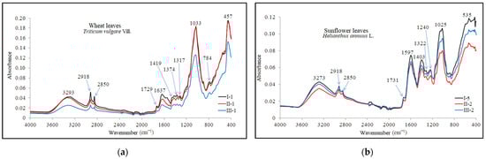
Figure 10.
ATR-FTIR characteristic spectra of (a) wheat and (b) sunflower leaves.
The plant tissues of the analyzed plants were found to contain several functional groups, including alkynes, alcohols, phenols, and amines I and II, identified by intense peaks in the area 3293 cm−1 and 3273 cm−1. These peaks are attributed to the stretching vibrations of groups such as ≡C-H, -(C)O-H, and -(C)-N-H [103]. The presence of lipids, proteins, carbohydrates, and nucleic acids was also indicated by strong peaks recorded at wave numbers 2918 cm−1 and 2850 cm−1, attributed to symmetric and asymmetric vibrations of carboxylic acids (-C=O) and alkanes (C-H). References [104,105,106] mention these groups at 2959–2852 cm−1, 2920 cm−1, and 2852 cm−1.
The wheat leaves exhibited more prominent peaks in comparison to those found in the sunflower leaves spectrum. The stretching vibration of the C=O group in the structure of carboxylic acids, phospholipids, hemicellulose, and pectin [106] was highlighted by the peak at 1733 cm−1. These compounds were identified in the spectra of analyzed wheat and sunflower leaves at wave numbers 1729 cm−1 and 1731 cm−1. These functional groups were also identified in the range of 1760–1680 cm−1 [105].
In the ATR-FTIR spectra of plant leaves, the absorption bands between 1650 and 1500 cm−1 range are attributed to the stretching vibrations of primary amines, proteins, lignins, and phenols. The peaks at 1637 cm−1 (wheat leaf) and 1597 cm−1 (sunflower leaf) signify the presence of primary amines. Additionally, the absorption band of 1470–1400 cm-1 range is attributed to the deformation vibration of C-OH and C-H groups found in polysaccharides, alcohols, carboxylic acids, and alkanes. The peaks at 1419 cm−1 (wheat leaf) and 1403 cm−1 (sunflower leaf) indicate the presence of these functional groups. Wave number 1317 cm−1 is attributed to the deformation vibration of the CH group in the cellulose structure and the stretching vibrations of C-OH groups in carboxylic acid and phenols. These peaks were observed in the ATR-FTIR spectrum at wave numbers 1317 cm−1 and 1322 cm−1. The absorption band at 1374 cm−1 is attributed to the deformation vibration of CH and H2C-H groups found in hemicellulose, xyloglucans, alkanes, phenols, and aliphatic structures. These clusters were detected at 1380–1350 cm−1 and 1371 cm−1 [103,105].
The region spanning from 1240 to 1033 cm−1 is indicative of polysaccharides, xyloglucans, and primary, secondary, and tertiary amines. The absorption bands in this range are associated with the stretching vibrations of the C-N, N-H, and C-O groups, as well as the deformation vibrations of the OH group within their structure [104,106]. Of particular note are the highly intense peaks at 1033 cm−1 in the wheat leaf spectrum and at 1025 cm−1 in the sunflower leaf spectrum.
Amines I and II, along with phenols, are identified in the spectrum obtained from wheat leaves by the average intensity peak at wave number 784 cm−1, which is associated with the deformation vibration of C-N-H and C-H groups. The presence of these groups is noted in the range of 900–660 cm−1 and 860–680 cm−1 [103]. Furthermore, the peak at wave number 535 cm−1, exclusive to the spectrum of sunflower leaves, is indicative of the stretching vibrations of the C-I and C-Br groups found in the alkyls within the plant’s structure.
In Figure A2, Appendix A, SEM micrographs (5000x), SEM-EDX spectra and elemental mapping of wheat and corn caryopsis, as well as sunflower achenes from various locations including TUL and SEN in GL County and VAD in BR County are presented. The micrographs depict the structural units of the plant tissues (membranes and cell walls) as well as organic compounds (lipids, starch, and proteins). Additionally, Table A2 (Appendix A), along with the EDX spectra and elemental distribution, revealed the presence of a number of 23 macro-, micro-, and trace elements in the grains and achenes, similar to those found in the soil. These findings underscore the strong relationship between soil mineralogy and plant composition. The grain tissue components with physiological activity are clearly marked and easily identifiable based on their morphology according to [107,108,109].
3.7. The Bioaccumulation of Elements in Crops
The Bioconcentration Factors (BFs) of soil heavy metals in crop plant leaves and caryopsis/achenes are shown in Figure 11 and Figure 12.
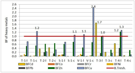
Figure 11.
Bioaccumulation factor of heavy metals in wheat and corn leaves and caryopsis.
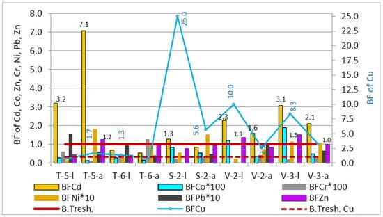
Figure 12.
Bioaccumulation factor of heavy metals in sunflower leaves and achenes.
The results indicate that, in the agroecological conditions of the studied area, wheat plants tend to exclude the bioaccumulation of Cd, Co, Cr, Ni, and Pb in their tissues. BFs for Cd ranged from 0.01 to 0.38 for leaves and from 0.0013 to 0.43 for caryopsis. BFs for Co were between 0.005 and 0.06 for leaves and from 0.0016 to 0.01 for caryopsis. The lowest BFs were observed for Cr (0.0024–0.03 for leaves and 0.0005–0.001 for caryopsis). BFs for Ni ranged between 0.02 and 0.12 for leaves and from 0.01 to 0.04 for caryopsis. BFs for Pb ranged from 0.05 to 0.10 for leaves and from 0.0017 to 0.14 for caryopsis. In contrast, for Zn and Cu, the bioaccumulation pattern was different. While the trend for the other elements was leaves > caryopsis, for Zn and Cu, it was to 0.14 for caryopsis. In contrast, for Zn and Cu, the bioaccumulation pattern was different. While the trend for the other elements was leaves > caryopsis, for Zn and Cu, it was caryopsis > leaves. BFs for Zn ranged from 0.43 to 0.62 for leaves and from 0.54 to 0.72 for caryopsis. The bioaccumulation of Cu was particularly pronounced in caryopsis, with BFs ranging from 0.23 to 1.09 for leaves and from 0.33 to 2.44 for caryopsis.
In the case of corn leaves and caryopses, the bioaccumulation factor for most elements was below one (the bioaccumulation threshold—B.Tresh.), indicating a limited capacity for phytoaccumulation under the ecological conditions in which the corn was grown. However, exceptions were observed for Cd, Zn, and Cu, with BFs exceeding one, suggesting a tendency for bioaccumulation of these elements in the leaves. Comparing the sections of the corn plant, the overall order of bioaccumulation was from leaf to caryopsis. Specifically, the BFs in leaves followed the order Cd (0.64–1.67) > Zn (1.00–1.23) > Cu (1.02–1.30) > Pb (0.16–0.41) > Ni (0.02–0.03) > Cr (0.0228–0.0229) > Co (0.005–0.009), while in caryopses, it was Zn (0.31–0.32) > Cd (0.03–0.21) > Cu (0.07–0.15) > Ni (0.0026–0.02) > Cr (0.0023–0.0052) > Co (0.0006–0.0010).
The results for sunflower BFs indicate that the bioconcentration of Cu, Cd, and Zn in both the leaves and achenes (seeds) is higher than that of other elements. The highest bioaccumulation values are observed for Cu, which in sampling sites S-2, V-2, and V-3 show the most significant accumulation. Specifically, for leaves, the bioaccumulation factor decreases in the order Cu (0.69–25.03) > Cd (0.68–3.19) > Zn (0.39–1.50) > Pb (0.0005–0.16) > Ni (0.01–0.12) > Co (0.0026–0.02) > Cr (0.0001–0.006), while for achenes, the order is Cd (0.53–7.07) > Cu (0.84–5.62) > Zn (0.83–1.24) > Ni (0.07–0.18) > Pb (0.04–0.09) > Cr (0.0010-0.0127) > Co (0.0013–0.0052).
Corn and sunflower, as high-biomass-producing plants, exhibit a notable capacity for the bioaccumulation of heavy metals in comparison to wheat. This study presents evidence indicating that corn and sunflower demonstrate a greater susceptibility for the bioextraction of copper, zinc, and cadmium.
3.8. Health Risk Assessment
The hazard quotient values corresponding to the three pathways of exposure (ingestion, dermal contact, and inhalation) indicate that there is no potential risk of adverse health effects for the adult population when exposed to Cr, Pb, Co, Zn, Cd, Ni, and Cu. The non-carcinogenic risks calculated for children also show no potential adverse effects from exposure to the investigated heavy metals, except for Cr. In two locations from Tulucesti and Vadeni, the dermal contact hazard quotient for Cr was greater than one (T-1—1.17, V-2—1.38), indicating a potential risk for adverse health effects in these areas.
According to the HQ results, it has been found that human exposure to Co may occur through ingestion for both adults (0.012–0.02) and children (0.15–0.32), but risk is negligible. On the other hand, exposure to Cr may occur through dermal contact and ingestion. The HQ for dermal and ingestion exposure in children is higher than that in the adult population. Specifically, the HQ for dermal exposure ranges from 0.40 to 1.38 for children and from 0.04 to 0.15 for adults. Similarly, the HQ for ingestion ranges from 0.28 to 0.95 for children and from 0.02 to 0.07 for adults. It is important to note that Pb, Zn, Cd, Ni, and Cu do not pose any hazardous risk for either children or adults. However, in Vadeni and some sites in Tulucesti (T-1, T-2, T-6), the HQ ingestion for Cu recorded very low levels (0.0003–0.00111 for adults and 0.00572–0.1475 for children).
The HI values for Co ranged from 0.01 to 0.02 for adults and from 0.15 to 0.32 for children. In contrast, Cr poses a higher risk of adverse health effects for children, with HI values ranging from 0.67 to 2.34, compared to 0.06 to 0.22 for adults. This suggests that children may be more vulnerable to exposure through ingestion, as they often put unwashed hands and objects they play with in their mouths. The health risk level by exposure to Cr and Co is presented in Figure 13.
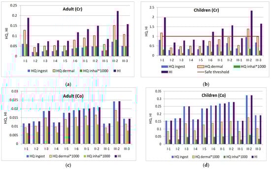
Figure 13.
Health risk through ingestion, dermal contact, and inhalation pathways: (a) chromium exposure of adults; (b) chromium exposure of children; (c) cobalt exposure of adults; and (d) cobalt exposure of children.
4. Conclusions
This research represents the first comprehensive investigation in the Galati–Braila region, SE Romania, focusing on the elemental, mineralogical, and microstructural analyses of soil and the three crop (wheat, corn, and sunflower) sections (leaves and caryopses/achenes) cultivated in SEN and TUL, GL County, and VAD, BR County areas.
It is the first scientific endeavor to evaluate the bioaccumulation capacity of major and trace elements in the plant tissues of wheat, corn, and sunflower using Bioaccumulation Factors (BFs) in the agroecosystems neighboring the Galati Iron and Steel Plant. Additionally, it contributes to the assessment of human health risks posed by topsoil dispersed particles.
The integrated analytical methods (HR-CS AAS, ATR-FTIR, SEM-EDX, PIGE) have proven to be valuable in identifying and quantifying environmental issues that might affect the population residing near the industrial facility.
The presence of heavy metals and other toxic substances from industrial and agricultural activities poses a threat to both the environment and human health. Our research has shown that the levels of Cr, Ni, Zn, and F exceed established Romanian safety standards and sometimes even surpassed the recommended intervention levels. These higher levels indicate a significant degree of contamination. The values of pollution indices highlighted the steel industry as the source of contamination. The investigated crops are crucial for human and animal consumption. Our findings showed that the concentration of heavy metals in crops is compartment- and plant-specific. For wheat and corn, the leaves contain higher levels of these elements compared to the seeds, while for sunflower, the pattern is the opposite.
Based on the hazard index (HI) values, it has been determined that chromium poses a risk of non-carcinogenic dermal contact and ingestion hazards, with children being particularly vulnerable to its adverse effects. On the other hand, the hazard index from cobalt through ingestion is considered to be minimal. Additionally, there is no potential risk of adverse health effects from exposure to lead (Pb), zinc (Zn), cadmium (Cd), nickel (Ni), and copper (Cu) for both adults and children.
The current lack of data on crop contamination and plant’s bioconcentration capacity in the Lower Danube Basin, near the metallurgical plant, makes it necessary to perform the following measures:
- − Implementation of comprehensive soil testing and continuous monitoring to proactively identify and address soil-to-plant contamination, preventing potential escalation;
- − Research on the contamination levels of other plant species grown for humans and animals feed in the steel industrial area;
- − Encouragement of farmers and stakeholders to prioritize the use of environmentally friendly fertilizers and pest control methods, while ensuring proper dosage according to soil properties and plant needs to mitigate potential risks associated with pollution;
- − Implementation of ongoing information and education programs for the population to prevent and combat ecosystem pollution.
These measures are crucial for environmental protection, public health preservation, and maintaining the overall ecological balance of the region.
This work may serve as a foundational framework for initiating innovative agropedological and plant physiology studies in the specific agricultural and ecological context of the southeastern region of Romania.
Author Contributions
Conceptualization, A.E. and S.S.M.; data curation, A.E. and S.S.M.; formal analysis, A.M.C.; investigation, A.E., S.S.M., D.I.M., A.P., S.G. and A.M.C.; methodology, A.E., S.S.M., D.I.M., A.P., S.G. and A.M.C.; project administration, A.E.; resources, A.E. and A.P.; software, S.S.M. and S.G.; validation, S.S.M. and D.I.M.; visualization, S.G.; writing—original draft, A.E. and S.S.M.; writing—review and editing, A.E., S.S.M., D.I.M., A.P., S.G. and A.M.C. All authors have read and agreed to the published version of the manuscript.
Funding
This research was funded by EC through JOP Black Sea Basin 2014–2020, project code BSB27-MONITOX (2018–2021).
Institutional Review Board Statement
Not applicable.
Informed Consent Statement
Not applicable.
Data Availability Statement
Data supporting reported results are available from the corresponding author upon request.
Acknowledgments
We acknowledge the support given by NIPNE team for technical support during PIGE analyses.
Conflicts of Interest
The authors declare no conflicts of interest.
Appendix A

Figure A1.
SEM-EDX spectrum of a soil sample and the elemental map distribution [1].
Figure A1.
SEM-EDX spectrum of a soil sample and the elemental map distribution [1].


Figure A2.
SEM-EDX spectra and elemental maps for selected vegetal compartments. (a) SEM-EDX spectrum of Triticum vulgare Vill. caryopsis and the elemental map distribution (large starch particle (g1), medium starch particle (g2), small starch particle (g3), protein matrix (mp), plasma membrane (pc)); (b) SEM-EDX spectrum of a Zea mays L. caryopsis and the elemental map distribution (small starch granule (g3), protein matrix (mp)); (c) SEM-EDX spectrum of cross-sectioned achenes of Helianthus annus L. and the elemental map distribution (lipid spherosomes (sl), cell membrane (mc), cell wall (pc)) [1].


Table A1.
Semi-quantitative EDX results of agricultural soil from TUL and SEN (GL) and VAD (BR) [1].
Table A1.
Semi-quantitative EDX results of agricultural soil from TUL and SEN (GL) and VAD (BR) [1].
| Elements | Tulucesti (TUL) | Sendreni (SEN) | Vadeni (VAD) | |||
|---|---|---|---|---|---|---|
| 0–5 cm | 5–30 cm | 0–5 cm | 5–30 cm | 0–5 cm | 5–30 cm | |
| Average Concentration (wt%) | ||||||
| C | 10.86 | 9.96 | 10.63 | 11.88 | 10.14 | 14.82 |
| N | 1.50 | * | * | * | * | 0.87 |
| O | 41.63 | 39.75 | 38.17 | 39.17 | 36.10 | 28.84 |
| Na | 0.45 | 0.38 | 0.58 | 0.39 | 0.40 | 0.62 |
| Mg | 1.32 | 1.54 | 1.31 | 1.46 | 1.07 | 1.03 |
| Al | 6.33 | 7.77 | 6.02 | 6.74 | 7.06 | 10.74 |
| Si | 23.83 | 22.60 | 22.44 | 20.84 | 25.28 | 26.27 |
| P | 0.26 | 0.24 | 0.10 | 0.15 | 0.26 | 0.16 |
| S | 0.09 | 0.02 | 0.09 | 0.10 | 0.19 | 0.04 |
| Cl | 0.07 | * | * | * | * | * |
| K | 2.59 | 3.33 | 1.63 | 1.77 | 3.57 | 3.43 |
| Ca | 3.58 | 3.64 | 4.67 | 6.26 | 1.69 | 2.69 |
| Ti | 0.55 | 0.55 | 0.43 | 0.55 | 0.65 | 0.88 |
| V | * | * | * | 0.20 | * | * |
| Cr | 0.23 | * | 0.35 | 0.19 | 0.49 | * |
| Mn | 0.27 | 0.47 | 0.40 | 0.51 | 0.67 | * |
| Gd | * | 1.46 | 1.33 | 0.87 | 1.59 | * |
| Fe | 4.04 | 5.08 | 4.02 | 5.07 | 5.52 | 8.35 |
| Co | 0.66 | 0.75 | 0.63 | 0.61 | 0.97 | 1.27 |
| Ni | 0.63 | 0.81 | 0.65 | 0.48 | 0.56 | * |
| Cu | * | * | 1.08 | 0.78 | 1.05 | * |
| Zn | 1.14 | 0.56 | 0.97 | 1.00 | 1.36 | * |
| Ga | * | 1.09 | 1.14 | 1.03 | 1.42 | * |
| Hg | * | * | 3.40 | * | * | * |
* Not detected.
Table A2.
Semi-quantitative EDX results for wheat and corn caryopsis and sunflower achenes collected from the target areas in Lower Danube Basin [1].
Table A2.
Semi-quantitative EDX results for wheat and corn caryopsis and sunflower achenes collected from the target areas in Lower Danube Basin [1].
| Elements | Triticum vulgare Vill. | Zea mays L. | Helianthus annuus L. |
|---|---|---|---|
| Average Concentration (wt%) | |||
| C | 59.76 | 65.65 | 74.61 |
| N | 3.50 | 2.60 | * |
| O | 24.80 | 23.18 | 18.49 |
| Na | 0.10 | 0.08 | 0.16 |
| Mg | 0.20 | 0.22 | * |
| Al | 0.20 | 0.27 | 0.06 |
| Si | 0.10 | 0.07 | * |
| P | 0.60 | 0.48 | * |
| S | 0.40 | 0.33 | * |
| Cl | 0.10 | 0.03 | * |
| K | * | 0.04 | 0.15 |
| Ca | 0.40 | 0.21 | 1.93 |
| Ti | * | 0.04 | 1.46 |
| V | * | 0.03 | * |
| Cr | 0.10 | 0.03 | 0.16 |
| Mn | 0.10 | 0.14 | * |
| Fe | 0.20 | 0.27 | * |
| Co | 0.30 | 0.18 | * |
| Ni | 0.30 | 0.60 | 0.19 |
| Cu | 0.90 | 1.18 | 0.17 |
| Zn | 0.80 | 0.66 | 0.09 |
| Pb | 6.18 | 3.71 | 2.57 |
| Hg | 1.24 | * | * |
* Not detected.
References
- Arbanas (Moraru), S.-S. Research on Iron and Steel Works Industry Impact on Soil Edaphic and Vegetal Potential in the Adjacent Areas (Cercetări Privind Impactul Activităţilor Industriei Siderurgice Asupra Potenţialului Edafic and Vegetal al Solurilor Din Zonele Adiacente—In Romanian). Ph.D. Thesis, Dunarea de Jos University of Galati, Galati, Romania, 2022. [Google Scholar]
- Wang, Y.; Xu, W.; Wang, Z.; Zhu, Y. The Impact of Vegetation Roots on Shallow Stability of Expansive Soil Slope under Rainfall Conditions. Appl. Sci. 2023, 13, 11619. [Google Scholar] [CrossRef]
- Blum, W.E.H. Functions of Soil for Society and the Environment. Rev. Environ. Sci. Bio/Technol. 2005, 4, 75–79. [Google Scholar] [CrossRef]
- Trap, J.; Bonkowski, M.; Plassard, C.; Villenave, C.; Blanchart, E. Ecological importance of soil bacterivores for ecosystem functions. Plant Soil 2016, 398, 1–24. [Google Scholar] [CrossRef]
- Jakubus, M.; Bakinowska, E. The Effect of Immobilizing Agents on Zn and Cu Availability for Plants in Relation to Their Potential Health Risks. Appl. Sci. 2022, 12, 6538. [Google Scholar] [CrossRef]
- Costa, C.; Lia, F. Temporal Variations of Heavy Metal Sources in Agricultural Soils in Malta. Appl. Sci. 2022, 12, 3120. [Google Scholar] [CrossRef]
- Zhou, B.; Zhang, T.; Wang, F. Microbial-Based Heavy Metal Bioremediation: Toxicity and Eco-Friendly Approaches to Heavy Metal Decontamination. Appl. Sci. 2023, 13, 8439. [Google Scholar] [CrossRef]
- Zhou, H.; Ouyang, T.; Guo, Y.; Peng, S.; He, C.; Zhu, Z. Assessment of Soil Heavy Metal Pollution and Its Ecological Risk for City Parks, Vicinity of a Landfill, and an Industrial Area within Guangzhou, South China. Appl. Sci. 2022, 12, 9345. [Google Scholar] [CrossRef]
- Ene, A.; Sloată, F.; Frontasyeva, M.V.; Duliu, O.G.; Sion, A.; Gosav, S.; Persa, D. Multi-elemental Characterization of Soils in the Vicinity of Siderurgical Industry: Levels, Depth Migration and Toxic Risk. Minerals 2024, 14, 559. [Google Scholar] [CrossRef]
- Alengebawy, A.; Abdelkhalek, S.T.; Qureshi, S.R.; Wang, M.-Q. Heavy Metals and Pesticides Toxicity in Agricultural Soil and Plants: Ecological Risks and Human Health Implications. Toxics 2021, 9, 42. [Google Scholar] [CrossRef]
- Pizzorno, J.; Pizzorno, L. Environmental Toxins Are a Major Cause of Bone Loss. Integr. Med. 2021, 20, 10–17. [Google Scholar]
- Pizzorno, J. Strategies for Protecting Mitochondria From Metals and Chemicals. Integr. Med. 2022, 21, 8–13. [Google Scholar] [PubMed]
- Alavanja, M.C.R.; Dosemeci, M.; Samanic, C.; Lubin, J.; Lynch, C.F.; Knott, C.; Barker, J.; Hoppin, J.A.; Sandler, D.P.; Coble, J.; et al. Pesticides and Lung Cancer Risk in the Agricultural Health Study Cohort. Am. Epidemiol. 2004, 160, 876–885. [Google Scholar] [CrossRef] [PubMed]
- Lamas, G.A.; Bhatnagar, A.; Jones, M.R.; Mann, K.K.; Nasir, K.; Tellez-Plaza, M.; Ujueta, F.; Navas-Acien, A. Contaminant Metals as Cardiovascular Risk Factors: A Scientific Statement from the American Heart Association. J. Am. Heart Assoc. JAHA 2023, 12, e029852. [Google Scholar] [CrossRef] [PubMed]
- Order of the Minister of Water, Forest and Environmental Protection No. 184/21.09.1997 for the Approval of the Procedure for the elaboration of Environmental Assessment, Official Monitor of Romania No. 303bis from 6.11.1997. (In Romanian). Available online: https://legislatie.just.ro/Public/DetaliiDocument/11971 (accessed on 25 May 2024).
- Benton Jones, J., Jr. Chapter 2. Field Sampling Procedures for Conducting a Plant Analysis. In Handbook of Reference Methods for Plant Analysis. Tissue Tests. Let Plant Speak; Kalra, Y.P., Ed.; CRC Press: Boca Raton, FL, USA, 1998; pp. 25–36. [Google Scholar]
- SR ISO 11466:1999; Soil Quality. Extraction of Trace Elements Soluble in Aqua Regia. International Organization for Standardization: Geneva, Switzerland, 1999.
- SR 7184/13:2001; Soils. Determination of pH in Water and Saline Suspensions (Mass/Volume) and in Saturated Paste. International Organization for Standardization: Geneva, Switzerland, 2001.
- STAS 7184/21-82; Soils. Determination of Humus Content. Engage in the European Research Infrastructures System: Bucharest, Romania, 1982.
- SR EN ISO 10693:2014; Soil Quality. Determination of Carbonate Content. Volumetric Method. International Organization for Standardization: Geneva, Switzerland, 2014.
- Borlan, Z.; Rauta, C. (Eds.) Methodology for Agrochemical Analysis of Soils to Establish the Need for Amendments and Fertilizers. Methods of Chemical Analysis of Soils; Methods, Guidance Reports Series; ICPA: Bucharest, Romania, 1981; Volume I, Part I. (In Romanian) [Google Scholar]
- SR ISO 11265+A1:1998; Soil Quality. Determination of the Specific Electrical Conductivity. International Organization for Standardization: Geneva, Switzerland, 1998.
- STAS 7184/7-87; Soils. Determination of Mineral Salts of 1:5 Aqueous Extract. Engage in the European Research Infrastructures System: Bucharest, Romania, 1987.
- STAS 7184/10-79; Soils. Determination of Granulometric Composition. Engage in the European Research Infrastructures System: Bucharest, Romania, 1979.
- SR ISO 11465:1998; Soil Quality. Determination of Dry Matter and Water Content on a Mass Basis. Gravimetric Method. International Organization for Standardization: Geneva, Switzerland, 1998.
- Caprita, F.-C.; Ene, A.; Cantaragiu Ceoromila, A. Valorification of Ulva rigida Algae in Pulp and Paper Industry for Improved Paper Characteristics and Wastewater Heavy Metal Filtration. Sustainability 2021, 13, 10763. [Google Scholar] [CrossRef]
- Ziegler, J.F.; Biersack, J.P. SRIM-2013 The Stopping and Range of Ions in Matter. 2013. Available online: http://srim.org/SRIM/SRIMLEGL.htm (accessed on 25 May 2024).
- Tesmer, J.R.; Nastasi, M. Handbook of Modern Ion Beam Materials Analysis; Materials Research Society: Pittsburg, PA, USA, 1995. [Google Scholar]
- GammaW Software. W. Westmeier, Version 2.70; Ebsdorfergrund-Mölln: Sprockhövel, Germany, 2015.
- Gomez, S.; Garcia, A.; Landete-Castillejos, T.; Gallego, L.; Pantelica, D.; Pantelica, A.; Preoteasa, E.A.; Scafes, A.; Straticiuc, M. Potential of the Bucharest 3 MV Tandetron™ for IBA studies of deer antler mineralization. Nucl. Instrum. Methods Phys. Res. 2016, B371, 413–418. [Google Scholar] [CrossRef][Green Version]
- Wang, C.; Xu, D.; Li, Y.; Zhou, W.; Bian, P.; Zhang, S. Source and Migration Pathways of Heavy Metals in Soils from an Iron Mine in Baotou City, China. Minerals 2024, 14, 506. [Google Scholar] [CrossRef]
- Wu, C.; Sun, B.; Tian, M.; Cheng, X.; Liu, D.; Zhou, Y. Enrichment Characteristics and Ecological Risk Assessment of Heavy Metals in a Farmland System with High Geochemical Background in the Black Shale Region of Zhejiang, China. Minerals 2024, 14, 375. [Google Scholar] [CrossRef]
- Jaskuła, J.; Sojka, M.; Fiedler, M.; Wróżyński, R. Analysis of Spatial Variability of River Bottom Sediment Pollution with Heavy Metals and Assessment of Potential Ecological Hazard for the Warta River, Poland. Minerals 2021, 11, 327. [Google Scholar] [CrossRef]
- Dou, C.; Cui, H.; Zhang, W.; Yu, W.; Sheng, X.; Zheng, X. Copper and Cadmium Accumulation and Phytorextraction Potential of Native and Cultivated Plants Growing around a Copper Smelter. Agronomy 2023, 13, 2874. [Google Scholar] [CrossRef]
- Yang, L.-Y.; Jiao, S.-L.; Wang, L.; Li, Y.-J.; Yang, M.; Feng, Y.-L.; Li, J.; Wei, Z.-X. Characteristics and Release Risk of Phosphorus from Sediments in a Karst Canyon Reservoir, China. Appl. Sci. 2024, 14, 2482. [Google Scholar] [CrossRef]
- Ahmed, F.; Fakhruddin, A.N.M.; Toufick Imam, M.D.; Khan, N.; Khan, T.A.; Rahman, M.M.; Abdulah, A.T.M. Spatial distribution and source identification of heavy metals pollution in roadside surface soil: A study of Dhaka Aricha highway, Bangladesh. Ecol. Process. 2016, 5, 2. [Google Scholar] [CrossRef]
- Caeiro, S.; Costa, M.H.; Ramos, T.B.; Fernandes, F.; Silveira, N.; Coimbra, A.; Medeiros, G.; Painho, M. Assessing heavy metal contamination in Sado Estuary sediment: An index analysis approach. Ecol. Indic. 2005, 5, 151–169. [Google Scholar] [CrossRef]
- Sutherland, R.A. Bed sediment-associated trace metals in an urban stream, Oahu, Hawaii. Environ. Geol. 2000, 39, 611–627. [Google Scholar] [CrossRef]
- Awadh, S.M.; Al-Hamdani, J.A.J.M.Z. Urban geochemistry assessment using pollution indices: A case study of urban soil in Kirkuk, Iraq. Environ. Earth Sci. 2019, 78, 587. 1–12. [Google Scholar] [CrossRef]
- Kowalska, J.B.; Mazurek, R.; Gąsiorek, M.; Zaleski, T. Pollution indices as useful tools for the comprehensive evaluation of the degree of soil contamination-A review. Environ. Geochem. Health 2018, 4, 2395–2420. [Google Scholar] [CrossRef] [PubMed]
- Műller, G. Index of geoaccumulation in sediments of the Rhine River. GeoJournal 1969, 2, 108–118. [Google Scholar]
- Nikolaidis, C.; Zafiriadis, I.; Constantinidis, T. Heavy Metal Pollution Associated with an Abandoned Lead-Zinc Mine in the Kirki Region, NE Greece. Bull. Environ. Contam. Toxicol. 2010, 85, 307–312. [Google Scholar] [CrossRef]
- Håkanson, L. An Ecological Risk Index for Aquatic Pollution Control: A Sedimentological Approach. Water Res. 1980, 14, 975–1101. [Google Scholar] [CrossRef]
- Pejman, A.; Bidhendi, G.N.; Ardestani, M.; Saeedi, M.; Baghvand, A. A new index for assessing heavy metals contamination in sediments: A case study. Ecol. Indic. 2015, 58, 365–373. [Google Scholar] [CrossRef]
- El-Alfy, M.A.; El-Amier, Y.A.; El-Eraky, T.E. Land use/cover and eco-toxicity indices for identifying metal contamination in sediments of drains, Manzala Lake, Egypt. Heliyon 2020, 6, e03177. [Google Scholar] [CrossRef]
- Long, E.R.; MacDonald, D.D.; Smith, S.; Calder, F.D. Incidence of Adverse Biological Effects Within Ranges of Chemical Concentrations in Marine and Estuarine Sediments. Environ. Manage. 1995, 19, 81–97. [Google Scholar] [CrossRef]
- Olowoyo, J.O.; van Heerden, E.; Fischer, J.L.; Baker, C. Trace elements in soil and leaves of Jacaranda mimosifolia in Tshwane area, South Africa. Atmos. Environ. 2010, 44, 1826–1830. [Google Scholar] [CrossRef]
- Mirecki, N.; Rukie Agič, R.; Šunić, L.; Milenković, L.; Ilić, Z.S. Transfer factor as indicator of heavy metals content in plants. Fresenius Environ. Bull. 2015, 24, 4212–4219. [Google Scholar]
- USEPA, California Department of Toxic Substances Control (DRSC), Office of Human and Ecological Risk (HERO), Human Health Risk Assessment (HHRA) Note Number 1: Recommended DTSC Default Exposure Factors for Use in Risk Assessment at California Hazardous Waste Sites and Permitted Facilities. 9 April 2019. Available online: https://dtsc.ca.gov/wp-content/uploads/sites/31/2022/02/HHRA-Note-1-April-2019-21A.pdf (accessed on 25 May 2024).
- Miletić, A.; Lučić, M.; Onjia, A. Exposure Factors in Health Risk Assessment of Heavy Metal(loid)s in Soil and Sediment. Metals 2023, 13, 1266. [Google Scholar] [CrossRef]
- Ackah, M. Soil elemental concentrations, geoaccumulation index, non-carcinogenic and carcinogenic risks in functional areas of an informal e-waste recycling area in Accra, Ghana. Chemosphere 2019, 235, 907–917. [Google Scholar] [CrossRef] [PubMed]
- Zheng, X.; Zhao, W.; Yan, X.; Shu, T.; Xiong, Q.; Chen, F. Pollution Characteristics and Health Risk Assessment of Airborne Heavy Metals Collected from Beijing Bus Stations. Int. J. Environ. Res. Public Health 2015, 12, 9658–9671. [Google Scholar] [CrossRef] [PubMed]
- Praveena, S.M.; Pradhan, B.; Aris, A.Z. Assessment of bioavailability and human health exposure risk to heavy metals in surface soils (Klang district, Malaysia). Toxin Rev. 2017, 37, 196–205. [Google Scholar] [CrossRef]
- Slaboch, J.; Malý, M. Land Valuation Systems in Relation to Water Retention. Agronomy 2023, 13, 2978. [Google Scholar] [CrossRef]
- Zhang, Z.; Chen, X.; Qin, X.; Xu, C.; Yan, X. Effects of Soil pH on the Growth and Cadmium Accumulation in Polygonum hydropiper (L.) in Low and Moderately Cadmium-Contaminated Paddy Soil. Land 2023, 12, 652. [Google Scholar] [CrossRef]
- Xu, F.; Vaziriyeganeh, M.; Zwiazek, J.J. Effects of pH and Mineral Nutrition on Growth and Physiological Responses of Trembling Aspen (Populus tremuloides), Jack Pine (Pinus banksiana), and White Spruce (Picea glauca) Seedlings in Sand Culture. Plants 2020, 9, 682. [Google Scholar] [CrossRef]
- Adamczyk-Szabela, D.; Wolf, W.M. The Impact of Soil pH on Heavy Metals Uptake and Photosynthesis Efficiency in Melissa officinalis, Taraxacum officinalis, Ocimum basilicum. Molecules 2022, 27, 4671. [Google Scholar] [CrossRef] [PubMed]
- Pikuła, D.; Stępień, W. Effect of the Degree of Soil Contamination with Heavy Metals on Their Mobility in the Soil Profile in a Microplot Experiment. Agronomy 2021, 11, 878. [Google Scholar] [CrossRef]
- Ahmad, I.; Malik, S.A.; Saeed, S.; Rehman, A.-u.; Munir, T.M. Phytoextraction of Heavy Metals by Various Vegetable Crops Cultivated on Different Textured Soils Irrigated with City Wastewater. Soil Syst. 2021, 5, 35. [Google Scholar] [CrossRef]
- Arbanas (Moraru), S.-S.; Ene, A. Nutrient stocks study in agroecosystems located near the steel industry, Galati, Romania. Ann. “Dunarea Jos” Univ. Galati Math. Phys. Theor. Mech. Fascicle II 2020, 43, 82–93. [Google Scholar] [CrossRef]
- Moraru, S.-S.; Ene, A.; Badila, A. Physical and Hydro-physical Characteristics of Soil in the Context of Climate Change. A Case Study in Danube River Basin, SE Romania. Sustainability 2020, 12, 9174. [Google Scholar] [CrossRef]
- Kabata-Pendias, A. Chapter 3. Soils and Soils Processes. In Trace Elements in Soils and Plants, 4th ed.; CRC Press: Boca Raton, FL, USA, 2011; pp. 37–63. [Google Scholar]
- Salminen, R.; Demetriades, A.; Reeder, S. Geochemical Atlas of Europe, Part I—Background Information, Methodology and Maps, FOREGS. Salminen, R., Ed.; 2005. Available online: http://www.gtk.fi/publ/foregsatlas (accessed on 25 May 2024).
- Dumitru, M.; Dumitru, S.; Tanase, V.; Mocanu, V.; Manea, A.; Vrânceanu, N.; Preda, M.; Eftene, M.; Ciobanu, C.; Calciu, I.; et al. Soil Quality Monitoring in Romania; Sitech: Craiova, Romania, 2011; pp. 51–59. [Google Scholar]
- Manea, A.; Dumitru, M.; Vrinceanu, N.; Eftene, A.; Anghel, A.; Vrinceanu, A.; Ignat, P.; Dumitru, S.; Mocanu, V. Soil heavy metal status from Maramureș county, Romania. In Proceedings of the GLOREP 2108 Conference, Timisoara, Romania, 15–17 November 2018. [Google Scholar]
- Pantelica, A.; Freitas, M.d.C.; Ene, A.; Steinnes, E. Soil pollution with trace elements at selected sites in Romania studied by instrumental neutron activation analysis. Radiochim. Acta 2013, 101, 45–50. [Google Scholar] [CrossRef]
- Order of the Minister of Water, Forest and Environmental Protection No. 756/3.11.1997 for the Approval of the Regulation Regarding the Assessment of the Environmental Pollution, Official Monitor of Romania No. 303bis from 06.11.1997. (In Romanian). Available online: https://legislatie.just.ro/Public/DetaliiDocument/13572 (accessed on 25 May 2024).
- Cullen, J.T.; Maldonado, M.T. Chapter 2. Biogeochemistry of Cadmium and Its Release to the Environment. In Cadmium: From Toxicity to Essentiality; Sigel, A., Sigel, H., Sigel, R.K.O., Eds.; Metal Ions in Life Science series; Spinger: Berlin/Heidelberg, Germany, 2013; Volume 11, pp. 31–62. [Google Scholar] [CrossRef]
- City of Hope. Available online: https://www.cancercenter.com/risk-factors/fluoride (accessed on 14 April 2024).
- Kumar, K.; Giri, A.; Vivek, P.; Kalaiyarasan, T.; Kumar, B. Effects of Fluoride on Respiration and Photosynthesis in Plants: An Overview. J. Res. Environ. Sci. Toxicol. JREST 2017, 2, 043–047. [Google Scholar] [CrossRef]
- Bhat, N.; Jain, S.; Asawa, K.; Tak, M.; Shinde, K.; Singh, A.; Gandhi, N.; Gupta, V.V. Assessment of Fluoride Concentration of Soil and Vegetables in Vicinity of Zinc Smelter, Debari, Udaipur, Rajasthan. J. Clin. Diagn. Res. 2015, 9, ZC63–ZC66. [Google Scholar] [CrossRef] [PubMed]
- WHO—World Health Organization. Preventing Disease through Healthy Environments. Inadequate or Excess Fluoride: A Major Public Health Concern, WHO/CED/PHE/EPE/19.4.5 (2019). Available online: https://apps.who.int/iris/handle/10665/329484 (accessed on 14 April 2024).
- Bulgariu, D.; Scarlat, A.A.; Bulgariu, L.; Astefanei, D.; Ciobanu, S.C. Chapter VIII. Considerations for carbonate analysis in soils. In Studies and Research in Geosciences; Rusu, C., Bulgariu, D., Eds.; “Al. I. Cuza” University: Iasi, Romania, 2018; Volume 2. (In Romanian) [Google Scholar]
- Moraru, S.-S.; Ene, A.; Gosav, S. Study of the correlativity between parameters and mineralogy of contaminated agricultural soils. In Proceedings of the 19th International Multidisciplinary Scientific Conference on Earth & Planetary Science—SGEM Geoconference, Albena, Bulgaria, 28 June–7 July 2019. [Google Scholar]
- Volkov, D.S.; Rogova, O.B.; Proskurnin, M.A. Organic matter and mineral composition of silicate soils: FTIR comparison study by photoacoustic, diffuse reflectance, and attenuated total reflection modalities. Agronomy 2021, 11, 1879. [Google Scholar] [CrossRef]
- Stoica, E.; Rauta, C.; Florea, N. (Eds.) Methods of Soil Chemical Analysis; The Agricultural Technical Propaganda Office: Bucharest, Romania, 1986; pp. 412–418. (In Romanian)
- Madejova, J.; Komadel, P. Baseline Studies of the Clay Minerals Society Source Clays: Infrared Methods. Clays Clay Miner. 2001, 49, 410–432. [Google Scholar] [CrossRef]
- Müller, C.M.; Pejcic, B.; Esteban, L.; Delle Piane, C.; Raven, M.; Mizaikoff, B. Infrared Attenuated Total Reflectance Spectroscopy: An Innovative Strategy for Analyzing Mineral Components in Energy Relevant Systems. Sci. Rep. 2014, 4, 6764. [Google Scholar] [CrossRef] [PubMed]
- Gosav, S.; Ene, A.; Aflori, M. Characterization and discrimination of plant fossils by ATR-FTIR, XRD and chemometric methods. Rom. J. Phys. 2019, 64, 806. [Google Scholar]
- Craciun, C. The study of some normal and abnormal montmorillonites by thermal analysis and infrared spectroscopy. Thermochim. Acta 1987, 117, 25–36. [Google Scholar] [CrossRef]
- Palacio, S.; Aitkenhead, M.; Escudero, A.; Montserrat-M, G.; Maestro, M.; Robertson, A.H.J. Gypsophile chemistry unveiled: Fourier Transform Infrared (FTIR) Spectroscopy provides new insight into plant adaptations to gypsum soils. PLoS ONE 2014, 9, e107285. [Google Scholar] [CrossRef] [PubMed]
- Mroczkowska-Szerszeń, M.; Orzechowski, M. Infrared spectroscopy methods in reservoir rocks analysis - semiquantitative approach for carbonate rocks. Nafta-Gaz 2018, 74, 802–812. [Google Scholar] [CrossRef]
- Sion, A.; Gosav, S.; Ene, A. ATR-FTIR qualitative mineralogical analysis of playground soils from Galati city, SE Romania. Ann. “Dunarea Jos” Univ. Galati Math.Phys. Theor. Mech. Fasc. II 2020, 43, 141–145. [Google Scholar] [CrossRef]
- Available online: https://ptable.com/#Properties/Series (accessed on 26 May 2024).
- Greger, M.; Landberg, T.; Vaculik, M. Silicon influences soil availability and accumulation of mineral nutrients in various plant species. Plants 2018, 7, 41. [Google Scholar] [CrossRef]
- Tubana, B.S.; Babu, T.; Datnoff, L.E. A Review of Silicon in Soils and Plants and Its Role in US Agriculture: History and Future Perspectives. Soil Sci. 2016, 181, 393–411. [Google Scholar] [CrossRef]
- Smical, A.I.; Hotea, V.; Oros, V.; Juhasz, J.; Pop, E. Studies on transfer and bioaccumulation of heavy metals from soil into lettuce. Environ. Eng. Manag. J. EEMJ 2008, 7, 609–615. [Google Scholar] [CrossRef]
- Krystofova, O.; Shestivska, V.; Galiova, M.; Novotny, K.; Kaiser, J.; Zehnalek, J.; Babula, P.; Opatrilova, R.; Adam, V.; Kizek, R. Sunflower Plants as Bioindicators of Environmental Pollution with Lead (II) Ions. Sensors 2009, 9, 5040–5058. [Google Scholar] [CrossRef]
- Gopal, R.; Khurana, N. Effect of heavy metal pollutants on sunflower. Afr. J. Plant Sci. 2011, 5, 531–536. [Google Scholar]
- Dhiman, S.S.; Zhao, X.; Li, J.; Kim, D.; Kalia, V.C.; Kim, I.-W.; Kim, J.Y.; Lee, J.-K. Metal accumulation by sunflower (Helianthus annuus L.) and the efficacy of its biomass in enzymatic saccharification. PLoS ONE 2017, 12, e0175845. [Google Scholar] [CrossRef] [PubMed]
- Mani, D.; Sharma, B.; Kumar, C.; Pathak, N. Phytoremediation potential of Helianthus annuus L. in sewage-irrigated Indo-Gangetic alluvial soils. Int. J. Phytoremediation 2012, 14, 235–246. [Google Scholar] [CrossRef] [PubMed]
- Commission Regulation (EC) No. 1181/2006 of 19 December 2006 Setting Maximum Levels of Certain Contaminants in Foodstuffs, Official Journal of European Union. L364 20.12.2006. p. 5. Available online: https://eur-lex.europa.eu/homepage.html (accessed on 25 May 2024).
- FAO/WHO, Codex Alimentarius—General Standard for Contaminants and Toxins in Food and feed, CXS 193-1995, (1995). Available online: https://www.fao.org/fao-who-codexalimentarius (accessed on 19 May 2024).
- Al-Othman, Z.A.; Ali, R.; Al-Othman, A.M.; Ali, J.; Habila, M.A. Assessment of toxic metals in wheat crops grown on selected soils, irrigated by different water sources. Arab. J. Chem. 2016, 9, S1555–S1562. [Google Scholar] [CrossRef]
- Directive 2002/32/EC of the European Parliament and of the Council of 7 May 2002 on Undesirable Substances in Animal Feed—Council statement, Official Journal of European Union, Official Journal of the European Communities, Chapter 3, Volume 42. L140/10 30.5.2002. Available online: http://data.europa.eu/eli/dir/2002/32/oj (accessed on 19 May 2024).
- Yang, Y.; Nan, Z.; Zhao, Z. Bioaccumulation and translocation of cadmium in wheat (Triticum aestivum L.) and maize (Zea mays L.) from the polluted oasis soil of Northwestern China. Chem. Spec. Bioavailab. 2014, 26, 1. [Google Scholar] [CrossRef]
- Alaboudi, K.A.; Ahmed, B.; Brodie, G. Phytoremediation of Pb and Cd contaminated soils by using sunflower (Helianthus annuus) plant. Ann. Agric. Sci. 2018, 63, 123–127. [Google Scholar] [CrossRef]
- Tegegne, W.A. Assessment of some heavy metals concentration in selected cereals collected from local markets of Ambo City, Ethiopia. J. Cereals Oilseeds 2015, 6, 8–13. [Google Scholar] [CrossRef]
- Shobha, N.; Kalshetty, B.M. Assessment of heavy metals in green vegetables and cereals collected from Jamkhandi local market, Bagalkot, India. Rasayan J. Chem. 2017, 10, 124–135. [Google Scholar] [CrossRef]
- Antoniadis, V.; Golia, E.E.; Lin, Y.-T.; Wang, S.-L.; Shaeen, S.M. Soil and maize contamination by trace elements and associated health risk assessment in the industrial area of Volos, Greece. Environ. Int. 2019, 124, 79–88. [Google Scholar] [CrossRef]
- Liang, J.; Chen, C.; Song, X.; Han, Y.; Liang, Z. Assessment of heavy metal pollution in soil and plants from Dunhua sewage irrigation area. Int. J. Electrochem. Sci. 2011, 6, 5314–5324. [Google Scholar] [CrossRef]
- Zehra, A.; Sahito, Z.A.; Tong, W.; Tang, L.; Hamid, Y.; Khan, M.B.; Ali, Z.; Naqi, B.; Yang, X. Assessment of sunflower germplasm for phytoremediation of lead-polluted soil and production of seed oil and seed meal for human and animal consumption. J. Environ. Sci. 2020, 87, 24–38. [Google Scholar] [CrossRef] [PubMed]
- Available online: https://specac.com/infrared-frequency-lookup/#frequencytool (accessed on 19 May 2024).
- Demir, P.; Onde, S.; Severcan, F. Phylogeny f cultivated and wild wheat species using ATR-FTIR spectroscopy. Spectrochim. Acta Part A Mol. Biomol. Spectrosc. 2015, 135, 757–763. [Google Scholar] [CrossRef] [PubMed]
- Utami, S.N.H.; Suswati, D. Chemical and spectroscopy of peat from West and Central Kalimantan, Indonesia in relation to peat properties. Int. J. Environ. Agric. Res. IJOEAR 2016, 2, 45–52. [Google Scholar]
- Gorgulu, S.T.; Dogan, M.; Severcan, F. The characterization and differentiation of higher plants by Fourier Transform Infrared Spectroscopy. Appl. Spectrosc. 2007, 61, 300–308. [Google Scholar] [CrossRef] [PubMed]
- Heneen, W.K.; Brismar, K. Scanning electron microscopy of nature grains of rye, wheat and triticale with emphasis on grain shrivelling. Hereditas 1987, 107, 147–162. [Google Scholar] [CrossRef]
- Shorstkii, I.A.; Zherlicin, A.G.; Li, P. Impact of pulse electric field and pulsed microwave treatment on morphological and structural characteristics on sunflower seed. Oilseeds Fats Crops Lipids OCL 2019, 26, 47. [Google Scholar] [CrossRef]
- Scheuer, P.M.; de Francisco, A.; de Miranda, M.Z.; Ogliari, P.J.; Torres, G.; Limberger, V.; Montenegro, F.M.; Ruffi, C.R.; Biondi, S. Characterization of Brazilian wheat cultivars for specific technological applications. Food Sci. Technol. 2011, 31, 816–826. [Google Scholar] [CrossRef][Green Version]


Disclaimer/Publisher’s Note: The statements, opinions and data contained in all publications are solely those of the individual author(s) and contributor(s) and not of MDPI and/or the editor(s). MDPI and/or the editor(s) disclaim responsibility for any injury to people or property resulting from any ideas, methods, instructions or products referred to in the content. |
© 2024 by the authors. Licensee MDPI, Basel, Switzerland. This article is an open access article distributed under the terms and conditions of the Creative Commons Attribution (CC BY) license (https://creativecommons.org/licenses/by/4.0/).