Location Selection Methods for Urban Terminal Co-Distribution Centers with Air–Land Collaboration

Abstract

Urban terminal logistics and distribution enterprises face the problems of duplicated network layouts, high costs, and inefficient urban environments. Recently, collaborative distribution using unmanned aerial vehicles (UAVs) and ground vehicles has been considered as a means of reducing costs and enhancing efficiency, thus overcoming the issues created by the high-density layout of enterprises’ relatively independent networks. This essentially involves constructing an air–ground collaborative common distribution network. To optimize the economic cost and distribution time of network operations, we established a site selection planning model for air–ground cooperative urban co-distribution centers and designed a solution method based on gray wolf optimization with K-means clustering. Taking the Wangsheren area of Jinan City, China, as an example, 15 UAV co-distribution centers and 13 vehicle co-distribution centers were identified. Although the average distribution cost of the network rose by 35–50% compared to traditional terminal distribution, the time saving was 80–85%, greatly improving the high-value-added service capacity. The end-distribution efficiency and customer satisfaction were also enhanced, which fully verifies the feasibility, validity, and applicability of the proposed model. Our approach can be applied to landing sites and the planning and optimization of large-scale commercial operations using logistics UAVs in urban areas.

1. Introduction

With the rapid development of online retail and e-commerce, there has been a surge in the demand for express delivery, imposing significant pressure on delivery enterprises to seize the market. Therefore, it is urgent to integrate duplicated outlets and improve the efficiency of single-point coordination and distribution. At the same time, the Civil Aviation Administration has promulgated “Civil Unmanned Aeronautics Development Roadmap V1.0” [1], which proposes that in 2025, urban short-distance, low-speed, lightweight, and small-scale terminal logistics and distribution scenarios will gradually mature and urban medium- and long-distance logistics and distribution will be gradually applied. The regularized operation of large distribution enterprises’ drone (unmanned aerial) logistics and distribution has already been realized, and the pilot distribution in various regions continues to advance, which will gradually realize the networked and scaled operation of drone distribution, thus causing a major change in the traditional express delivery system, network structure, and transportation mode. Based on the integration needs of scattered outlets, combined with drone distribution means, an intensive, multi-mode common distribution network integrating drone distribution will be built, which has a greater social and application value for improving the quality and efficiency of end distribution. Among them, the key to the rational operation of this cooperative co-distribution network is the siting of the co-distribution center, and the rationality of the siting layout scheme is crucial to the network cost and operational efficiency, but there are few research results on the siting of co-distribution centers integrating drones. So, in order to solve the aforementioned problems and provide a theoretical basis for the field of drone co-distribution research, this paper researches the siting of the urban end co-distribution center with air–ground cooperation. This paper also researches the air–land cooperative urban terminal co-distribution center-siting method and proposes a co-distribution center-siting point solution method based on regional demand points. Section 2 introduces the current research status of UAV and ground distribution. Section 3 introduces the model of UAV and ground co-distribution. Section 4 introduces the model solution method based on the GWO algorithm. In Section 5, the effectiveness and computational efficiency of the algorithm are verified through experiments. Section 6 is the conclusion of this article.

2. State of the Art

To date, research on common distribution networks has mainly focused on traditional ground distribution facilities, and most of them carry out theoretical modeling with distribution timeliness and economy as the main objectives. Özmen M. pointed out the regional characteristics of logistics centers (which are used to perform regional logistics activities, such as storage, transportation, and infrastructure services, and whose layout planning is affected by cost and benefit issues), proposed the three-phase method for solving the location of logistics centers, and analyzed the robustness of the algorithm [2]. Mousavi S. M. et al. proposed cross-docked logistics and transportation modes, and for this type of logistics and distribution modes, a modern multi-criteria group decision making (MCGDM) model was proposed to solve the results of calculating the layout of cross-docked logistics centers [3]. Ji et al. first used the K-means clustering algorithm, customer clustering, to solve pickup and delivery point siting and customer group division [4]. Next, on the basis of the optimal solution, they built a single-vehicle-yard multi-model collection and distribution integrated VRP model using a scanning algorithm and an ant colony algorithm to solve the problem of vehicle distribution routes [4]. Cui comprehensively investigated factors influencing the operating costs and resilience of the network based on common distribution and the integration and reorganization of courier terminal distribution resources and established a courier terminal common distribution service center multi-objective siting model [5]. Based on complex network theory to determine the importance of alternative nodes, Bi established a multi-objective siting model for the urban express terminal crowdsourcing service station by considering three objectives, namely the enterprise operation cost, customer satisfaction, and carbon emission, and proposed a genetic algorithm for model solving [6]. These studies provide a theoretical basis for the distribution center-siting problem, but none of them consider the convergent siting of UAV distribution centers.

Research related to the siting of UAV logistics and distribution facilities has mainly considered pure UAV airport siting. Shavarani S. M. et al. argued that drone logistics is an important avenue for surface traffic congestion and developed a landing site-siting model that targeted the total cost, took into account drone endurance and multiple takeoff and landing facilities, and validated it using San Francisco as a case study [7]. Venkatesh et al. concluded that mixed-integer programming performs well in the generalized facility-siting problem and used mixed-integer programming to optimize the siting of logistics drone vertical-landing sites with and without capacity constraints [8]. Brian et al. examined vertical-takeoff and vertical-landing electric UAVs and considered multiple distribution modes. They optimized the siting of takeoff and landing locations under the premise of a restricted number of such sites to maximize demand coverage [9]. Ren et al. focused on the airport-siting problem of UAV urban instant delivery and established a mixed-integer planning model for UAV fully automated airport siting. They used the improved regular grid method for pre-siting and optimized the solution through Tyson partitioning [10]. Lu et al. established a two-layer planning model for the site–path optimization of UAV delivery relay stations on islands and combined K-means clustering with an improved simulated annealing algorithm to solve the problem [11]. Qian et al. introduced airspace environmental constraints in establishing their multilevel-logistics UAV landing point site selection and allocation model [12,13]. Fabio Borghetti et al. designed a drone delivery service system based on drone delivery preference survey data and evaluated the benefits of the delivery enterprise through preliminary financial analysis. The results showed that drone last-mile delivery is suitable for small and lightweight packages, which can effectively reduce the impact on the environment and society and safeguard the profit of the enterprise [14].

In this paper, a model of ground and UAV co-distribution is innovatively established and a solution method is provided. This model can give full play to the advantages of the two distribution methods and ensure that the economic benefits are maximized under the premise of the shortest distribution time in the region.

3. Modeling

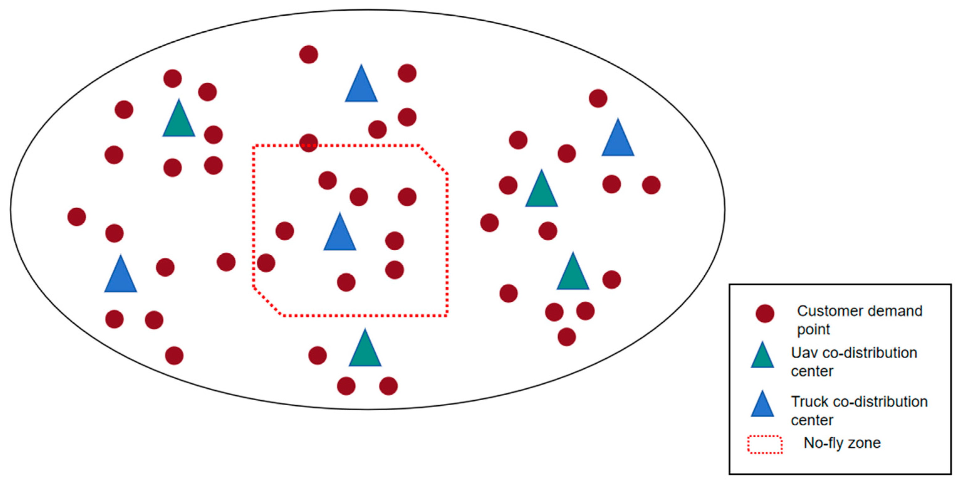
3.1. Problem Description

According to the terminal distribution demand points in a certain urban area, two types of co-distribution centers are set up, namely air and ground. The associated distribution tasks are accomplished by UAVs and land-based vehicles, respectively. Through the connection between co-distribution centers and terminal stations or other intelligent receiving points, full coverage of regional distribution demand points is realized. To minimize the construction and operation costs of the regional distribution network and the overall distribution time, the site layout of the distribution centers must be optimized. This paper proposes a method for determining the optimal combination of air–ground cooperative distribution centers. Airspace management requirements are fully considered, and certain no-fly zone restrictions are set within the study area to improve the applicability of the planning method. Figure 1 shows a schematic diagram of the model’s proposed solution scenarios and problems.

3.2. Assumptions

Based on the problem description, the following assumptions are made:

• The information of all customer demand points is known.
• After the number and location of the co-distribution centers are determined, the UAV distribution flight routes and vehicle travel routes are fixed. All routes start from a co-distribution center and return to the center after completing the customer distribution service.
• The distribution capacity of the two types of co-distribution centers is fixed.
• The cost of UAVs is mainly considered in the flight process, not in the hovering state.
• Sufficient energy (fuel) is maintained during the transportation of both UAVs and vehicles, without considering the time required for UAVs to take off, land, recharge and change the power source, and load and unload cargo.
• UAVs and vehicles fly and travel at a uniform speed.

3.3. Notation

The variables in the planning and layout model of the air–ground cooperative co-distribution center are defined in

Table 1. Explanation of symbols related to the planning and layout model of the air–ground cooperative co-distribution center.

Symbol Type	Notation Expression	Meaning
Collections	I = {1, 2, 3,……n}	Collection of an alternative co-distribution center
	J = {1, 2, 3,……m}	Collection of customer demand points
	S = {1, 2}	Categorized collection of co-distribution centers
	U = {1, 2, 3,……u}	Collection of UAVs
	K{1, 2, 3,……k}	Collection of vehicles
Subscripts	i ∈ I	Subscript of alternative co-distribution centers
	j ∈ J	Subscript of customer demand points
	s ∈ S	Subscript of co-distribution center types
	u ∈ U	Subscript of UAVs
	k ∈ K	Subscript of vehicles
Parameters	α	Time function weights
	β	Cost function weights
	hj	Distribution demand at demand point j
	Es	Service capacity of the co-distribution centers
	Qu	Maximum load capacity of the UAV (kg)
	quij	Single-delivery capacity of the UAV (kg)
	Qk	Maximum load capacity of the vehicle (kg)
	qkij	Single-delivery capacity of the vehicle (kg)
	Ru	Maximum service distance of UAV co-distribution centers (km)
	Rk	Maximum service distance of vehicle co-distribution centers (km)
	Du	Maximum range of the UAV (km)
	Dk	Maximum range of the vehicle (km)
	vu	Average delivery speed of the UAV (km/h)
	vk	Average delivery speed of the vehicle (km/h)
	Cs	Construction cost of the co-distribution center (CNY)
	duij	Flight distance of the UAV from co-distribution center i to customer demand point j (km)
	dkij	Distance of the vehicle from co-distribution center i to customer demand point j (km)
	Cuv	Distribution and operating costs of the UAV co-distribution center (CNY/pc)
	Ckv	Distribution and operating costs of the UAV co-distribution center (CNY/pc)
Variants	xis	Whether the alternative landing site i is to be constructed as an s-type co-distribution center, with a value of 1 for yes and 0 for no
	yuij	Whether customer demand point j is delivered by UAV co-distribution point i, with a value of 1 for yes and 0 for no
	ykij	Whether customer demand point j is delivered by vehicle co-distribution point i, with a value of 1 for yes and 0 for no
	Aij	Whether the distribution path between UAV co-distribution point i and customer demand point j crosses the no-fly zone, with a value of 1 for no and 0 for yes

.

3.4. Model Construction

Considering the service capacity and coverage of the different types of co-distribution centers and with the goal of minimizing the total cost of network operations and the overall distribution time, a multi-objective planning and layout model is constructed.

$$\min Z=\alpha {\displaystyle \sum Z_{time}}+\beta {\displaystyle \sum Z_{cost}}$$

(1)

$${\displaystyle \sum Z_{time}}={\displaystyle \sum _{u=1}^a{\displaystyle \sum _{i=1}^n{\displaystyle \sum _{j=1}^m\frac{d_{ij}^u}{v_u}}}}\cdot y_{ij}^u+{\displaystyle \sum _{k=1}^b{\displaystyle \sum _{i=1}^n{\displaystyle \sum _{j=1}^m\frac{d_{ij}^k}{v_k}}}}\cdot y_{ij}^k$$

(2)

$${\displaystyle \sum Z_{cost}}={\displaystyle \sum _{s=1}^2{\displaystyle \sum _{i=1}^n{C}_s\cdot x_{is}}}+{\displaystyle \sum _{s=1}^2}{\displaystyle \sum _{i=1}^n{\displaystyle \sum _{j=1}^m(c_v^u{y}_{ij}^u+}}{c}_v^k{y}_{ij}^k)\cdot x_{is}$$

(3)

$${\displaystyle \sum _{i=1}^n{\displaystyle \sum _{s=1}^2{x}_{is}\le n}}$$

(4)

$${\displaystyle \sum _{s=1}^2{x}_{is}\le 1}$$

(5)

$${\displaystyle \sum _i^n{y}_{ij}=1},\forall j\in J$$

(6)

$${\displaystyle \sum _{i=1}^n}{\displaystyle \sum _{j=1}^m(y_{ij}^u+y_{ij}^k)}{h}_j\le {\displaystyle \sum _{s=1}^2{x}_{is}}{E}_s,\forall i\in I$$

(7)

$$A_{ij}-y_{ij}^u\ge 0\hspace{1em}\forall i\in I,\forall j\in J$$

(8)

$$A_{ij}{y}_{ij}^u{d}_{ij}^u\le \frac{D_u}{2}\hspace{1em}\forall i\in I,\forall j\in J,\forall u\in U$$

(9)

$$q_{ij}^u\le Q_u\hspace{1em}\forall i\in I,\forall j\in J$$

(10)

$$q_{ij}^k\le Q_k\hspace{1em}\forall i\in I,\forall j\in J$$

(11)

$$A_{ij}{y}_{ij}^u{d}_{ij}^u\le R_u\le \frac{D_u}{2}\hspace{1em}\forall i\in I,\forall j\in J,\forall u\in U$$

(12)

$$y_{ij}^k{d}_{ij}^k\le R_k\le \frac{D_k}{2}\hspace{1em}\forall i\in I,\forall j\in J,\forall k\in K$$

(13)

$$y_{ij}^u+y_{ij}^k\le {\displaystyle \sum _{s=1}^2{x}_{is}}\hspace{1em}\forall i\in I,\forall j\in J,\forall s\in S$$

(14)

In the model, Equation (1) is the overall objective function of the mixed-integer planning. Equation (2) is the distribution time function, including the total time for UAVs and vehicles to complete the distribution task, and Equation (3) is the cost function, which includes the construction cost of warehouses, facility renovation, and platform construction, as well as distribution costs, such as the cost of the purchase of facilities and equipment, energy consumption, human resources, and equipment maintenance. Equation (4) imposes a constraint on the number of landing points, i.e., the total number of co-distribution centers cannot exceed the number of alternative co-distribution centers. Equation (5) states that any alternative co-distribution center must be either an air or a ground center. Equation (6) is a constraint on the matching of supply and demand points (i.e., for any demand point, there is only one co-distribution center responsible for the distribution) and prevents the existence of demand points that cannot be distributed or distribution locations with more than one point of departure and landing. Equation (7) is the capacity–demand matching constraint, i.e., for any alternative co-distribution center, if selected, its capacity must exceed the volume of distribution services. Equation (8) is the no-fly-zone constraint for the alternative co-distribution center and the demand point, i.e., if the straight line between the two endpoints of the flight path crosses the no-fly zone, then the distribution relationship is invalid. Equations (9) and (10) impose performance constraints on the UAVs, such that the weight of the distribution goods cannot exceed the maximum UAV load. Equation (11) is a distribution vehicle performance constraint, specifying that the weight of the distribution goods cannot exceed the maximum load of the logistics vehicles. Equations (12) and (13) are service distance constraints, i.e., for any type of co-distribution center, the actual distribution distance must be less than the maximum distance of its service and less than half of the performance mileage of the distribution mode. Equation (14) is the distribution relationship constraint, i.e., when a point is selected as a co-distribution center, there must be a distribution relationship between the co-distribution center and the demand point.

4. Algorithm Design

Due to its discrete nature, constraint diversity, and multi-objective optimization, the site selection problem is difficult to solve in polynomial time, and thus, it is essentially an NP problem. This is especially true for the co-matching model proposed in this paper, where the complexity of the functions in the model, the large size of the problem, and the diversity of constraints determine that it is not suitable to be solved by an exact algorithm [15]. Using heuristic algorithms for solving is a proven method.

As an innovative bio-heuristic optimization algorithm, the gray wolf optimization algorithm solves complex optimization problems by imitating the social hierarchy and hunting behavior of gray wolves; shows excellent global optimization-seeking ability, strong exploratory power, and adaptability in dealing with multidimensional NP problems; and can adapt well to the various constraints in the site selection problem in terms of population initialization and updating strategies. Compared with other heuristic algorithms, the gray wolf algorithm has a fast convergence speed, a high solution rate, a strong global exploration ability, and high stability, with simple implementation, which makes it an ideal choice for solving combinatorial optimization problems, such as site selection and layout [16]. In recent years, the gray wolf algorithm has been widely used to solve unconstrained, constrained, and multi-objective NP problems in engineering, healthcare, and environment [15,17,18,19,20,21,22].

Therefore, this paper proposes a two-stage site selection solution algorithm. First, based on K-means clustering, alternative point sets for co-location center siting are calculated by demand points; next, the optimal solution for siting that satisfies the constraints is selected from the co-location center selection set by using the gray wolf optimization algorithm.

4.1. Construction of a Co-Distribution Center Preselection Set Based on K-Means Clustering

According to center ground theory and the concept of hexagonal network systems, when end outlets with different service capabilities are arranged, the service scope forms a hexagonal service area in the center ground, covering the whole demand area. Combined with the size of the actual service radius of express delivery outlets, this provides the initial set of distribution areas [23]. Taking the number of proposed outlets as the classification number, the set of co-distribution centers can be selected from the demand points using K-means clustering [24]. According to the model specified in Section 3.4, the set of demand points is J, the target classification number of the clustering algorithm is k, and the preselected set of co-distribution centers is I. Let I_n be the n-th point of this set. The process of selecting the distribution center from the preselected set using K-means clustering is as follows.

Step 1: Randomly select a point from all customer demand points as the first point of the preselected set of co-distribution centers:

$$I_1=Random(J), J=\{1,2,3,\dots ,m\}$$

(15)

Step 2: Calculate the minimum distance of each remaining customer demand point from the preselected set of identified co-distribution centers:

$$D(J_l)=\underset{l\in J,k\in I}{\min }\sqrt{{(x_{J_l}-x_{l_k})}^2+{(y_{J_l}-y_{l_k})}^2}$$

(16)

Step 3: Calculate the probability that each demand point will be selected as the next clustering center, and select that with the highest probability as a new preselected point for the co-distribution center:

$$P(J_l)=\frac{D(J_l)}{{{\displaystyle \sum D(J_l)}}^2}$$

(17)

$$I_{j+1}=J_s|s=\underset{s\in J}{\max }P(J_l)$$

(18)

$$I=I\cup I_{j+1}, j=j+1$$

(19)

Step 4: If j = k, terminate the operation and return I as the final result, i.e., the preselected set of co-distribution centers; otherwise, return to step 2.

After performing the aforementioned process, the clustering algorithms for different numbers of target categories were evaluated, and the final classification values and preselected set of co-distribution centers were determined [25].

4.2. Co-Distribution Center Site Selection Method Based on GWO

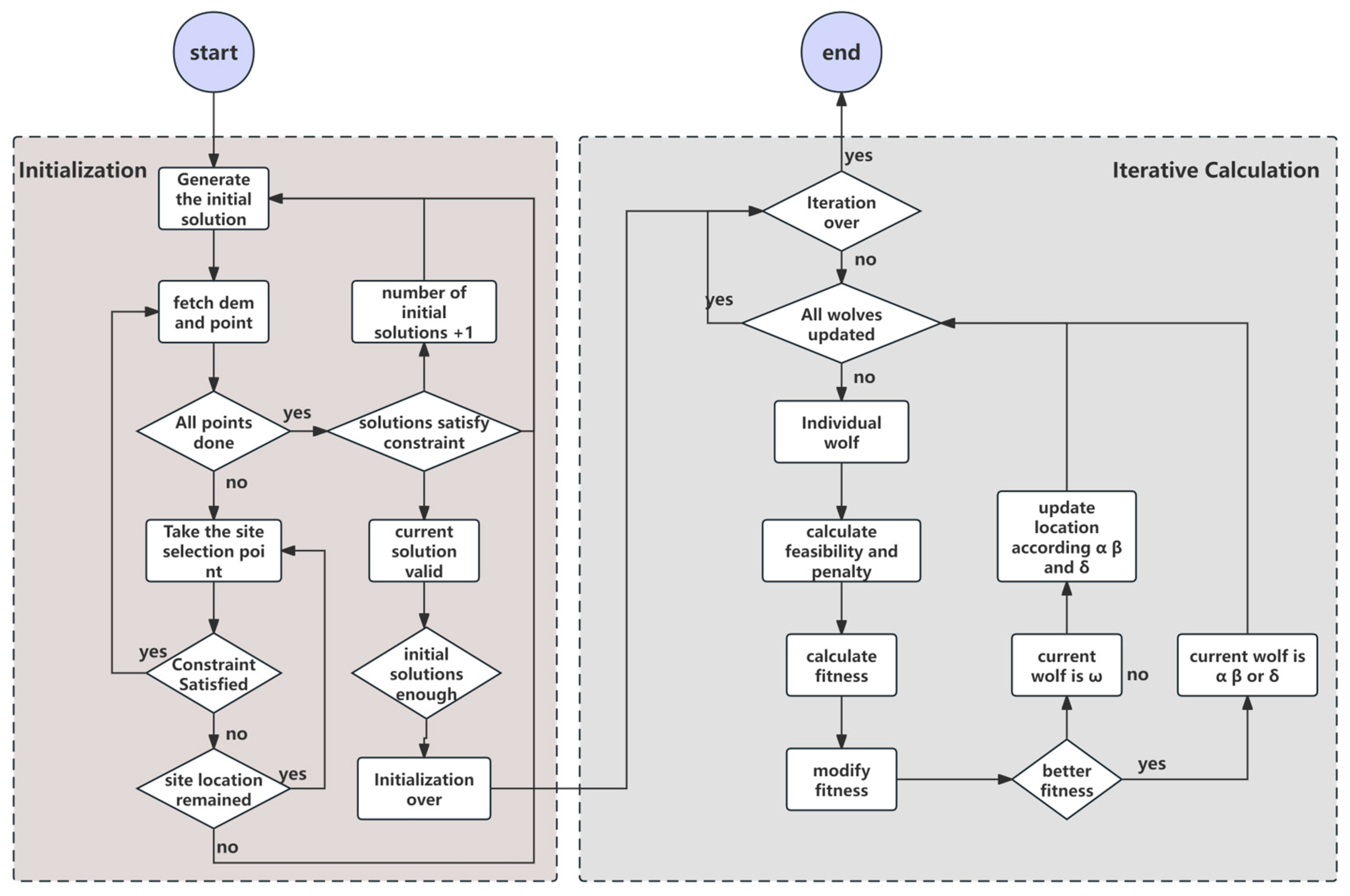
4.2.1. Algorithm Flow

The wolf pack was first initialized to generate a set of effective initial solutions. The main iterative computation was carried out to explore and optimize the generated solutions, and the optimal solutions were used as the final set for site selection. The algorithm flow is illustrated in Figure 2, and the pseudocode for solving the problem is presented in

Table 2. Pseudocode of the site selection method based on GWO.

Initialization: 1. Initialize the size of the gray wolf pack, N (i.e., the number of solutions). 2. Randomly initialize the position of each gray wolf $X_i(i=1,2,\cdots ,N)$, where each position represents a potential site solution. 3. Initialize $\alpha$, $\beta$, and $\delta$ as the best three solutions in the population. 4. Set the maximum number of iterations as MaxIteration and the current iteration as iter = 0.

Iteration starts: While iter < MaxIteration do  for each wolf i in Pack do    1. Calculate the feasibility and penalty of the solution $Feasible(i)$ and $Penalty(i)$    2. Calculate $Fitness(i)$.    3. Modify the fitness based on the results in steps 1 and 2    4. Locate the best three wolves based on $\alpha$, $\beta$, and $\delta$    5. Calculate the distances of the other wolves in the pack from $\alpha$, $\beta$, and $\delta$ according to $\left|\overrightarrow{C_1}\cdot \overrightarrow{X_{\alpha }}-\overrightarrow{X}\right|$, $\left|\overrightarrow{C_2}\cdot \overrightarrow{X_{\beta }}-\overrightarrow{X}\right|$, and $\left|\overrightarrow{C_3}\cdot \overrightarrow{X_{\delta }}-\overrightarrow{X}\right|$    6. Calculate new positions around $\alpha$, $\beta$, and $\delta$ as $\overrightarrow{X_1}$, $\overrightarrow{X_2}$, and $\overrightarrow{X_3}$    7. Update the position of the wolves $\overrightarrow{X}(t+1)=\frac{\overrightarrow{X_1}+\overrightarrow{X_2}+\overrightarrow{X_3}}{3}$, where $\overrightarrow{X_k}=\overrightarrow{X_{\alpha }}-\overrightarrow{A_k}\cdot \left|\overrightarrow{C_k}\cdot \overrightarrow{X_{\alpha }}-\overrightarrow{X}\right|, k\in 1,2,3$    8. Apply rounding according to Equation (21) and truncation according to Equation (22)   $endfor$   9. Check for new $\alpha$, $\beta$, and $\delta$   10. Update the coefficients a, A, and C, which control the search behavior of the wolves, decreasing as the iteration proceeds   11. iter = iter + 1 end while

Output: Location of $\alpha$ as the best siting option.

.

4.2.2. Processing of Site Selection Data

The set of alternative points for the co-distribution center is $\overrightarrow{I}=[I_1,I_2,\cdots ,I_n]$. Each point $I_k$ is evaluated according to

$$\left\{\begin{array}{l}{I}_k=1,\mathrm{not}\mathrm{constructed}\\ I_k=2,\mathrm{constructed}\mathrm{as}\mathrm{UAV}\mathrm{center},k\in n\\ I_k=3,\mathrm{constructed}\mathrm{as}\mathrm{Truck}\mathrm{center}\end{array}\right.$$

(20)

In the traditional GWO algorithm, all computations are performed in the real number domain, and solutions are generally continuous in the real number space [26]. However, in the site selection problem, when updating the wolf positions, non-integer solutions may be generated, and these cannot be directly used for site selection. Therefore, these solutions must be processed so that they conform to the form specified in Equation (20) for the computational needs of the site selection problem.

The position vector $\overrightarrow{X}$ is rounded as follows to generate a new position vector $\overrightarrow{X\_I}$:

$$\overrightarrow{X\_I}=round(\overrightarrow{X})$$

(21)

If any element in $\overrightarrow{X\_I}$ does not satisfy Equation (20), further truncation is applied according to

$${\overrightarrow{X\_I}}_m=\left\{\begin{array}{l}{\overrightarrow{X\_I}}_m=1,{\overrightarrow{X\_I}}_m\le 1\\ {\overrightarrow{X\_I}}_m=2,1<{\overrightarrow{X\_I}}_m\le 2\\ {\overrightarrow{X\_I}}_m=3,3\le {\overrightarrow{X\_I}}_m\end{array}\right.,m\in K$$

(22)

4.2.3. Initialization Strategies for Wolf Packs

In the starting phase, a batch of initial solutions representing the positions of the wolf pack members is generated by random selection. This enhances the population diversity of the wolf pack and, thus, its exploration efficiency. Taking a single alternative search point $I_k$ as an example, its initial value at time $t_0$ is

$$I_k{t}_0=rand(1,2,3)$$

(23)

In the initial solution, the alternative points are randomized in terms of which type of co-distribution center they are. The set of alternative co-distribution center points is

$$I(t_0)=[I_1(t_0),I_2(t_0),\cdots ,I_k(t_0),\cdots ,I_n(t_0)]$$

(24)

To improve the convergence speed of the algorithm and the possibility of finding a global optimal solution, the initial solution should be of high quality. This subsection describes an initial solution computation method that eliminates meaningless initial solutions under the premise of random generation.

Step 1: Generate a random initial solution set $I(t_0)$ according to Equation (24), and set $I^{*}=I(t_0)$.

Step 2: Set j = 1.

Step 3: Determine whether customer demand point j satisfies the constraint. If so, continue to step 4; otherwise, jump to step 5.

Step 4: Set j = j + 1. If j = MaxDemandPointNumber, jump to Step 8; otherwise, return to step 3.

Step 5: Check whether there is any alternative set point for UAV or truck co-distribution centers that has not been planned. If so, continue to step 6; otherwise, jump to step 7.

Step 6: Randomly select the point $k^{\prime }$ that satisfies $I_k(t_0)=1$, and reassign $I_{k^{\prime }}(t_0)=rand(2,3)$ so that $I^{*}=I^{{*}^{\prime }}$; return to step 2.

Step 7: Randomly select the point $k^{\prime }$ that satisfies $I_k(t_0)=2$, and reassign $I_{k^{\prime }}(t_0)=3$ so that $I^{*}=I^{{*}^{\prime }}$; return to step 2.

Step 8: Terminate the process.

4.2.4. Design of the Fitness Function

In the process of selecting co-distribution center sites, it is necessary to consider the optimization of two key indicators, cost and delivery time. The aim is to simultaneously minimize these indicators, as specified by Equation (1). For this purpose, the following fitness function is set:

$$fitness={\omega }_t{f}_{time}+{\omega }_c{f}_{cost}$$

(25)

where f_time is described in Equation (26) and f_cost is described in Equation (27). For both functions, smaller values are preferable.

$$f_{time}=\frac{\max Z_{time}-Z_{time}}{\max Z_{time}-\min Z_{time}}$$

(26)

$$f_{cost}=\frac{\max Z_{cost}-Z_{cost}}{\max Z_{cost}-\min Z_{cost}}$$

(27)

In Equation (26), the maximum distribution time $\max Z_{time}$ occurs when all co-distribution centers are of ground type and each customer demand point is distributed by the farthest distribution center. The minimum distribution time is 0, satisfying $f_{time}\in \left(0\right.\left.,1\right]$. Similarly, in Equation (27), the maximum cost $\max Z_{cost}$ occurs when all co-distribution centers are of air type and each customer demand point is distributed by the farthest distribution center. The minimum cost is 0, satisfying $f_{cost}\in \left(0\right.\left.,1\right)$. The scaling coefficients ${\omega }_t$ and ${\omega }_c$ in Equation (25) ensure that the two indicators can be considered in a balanced way.

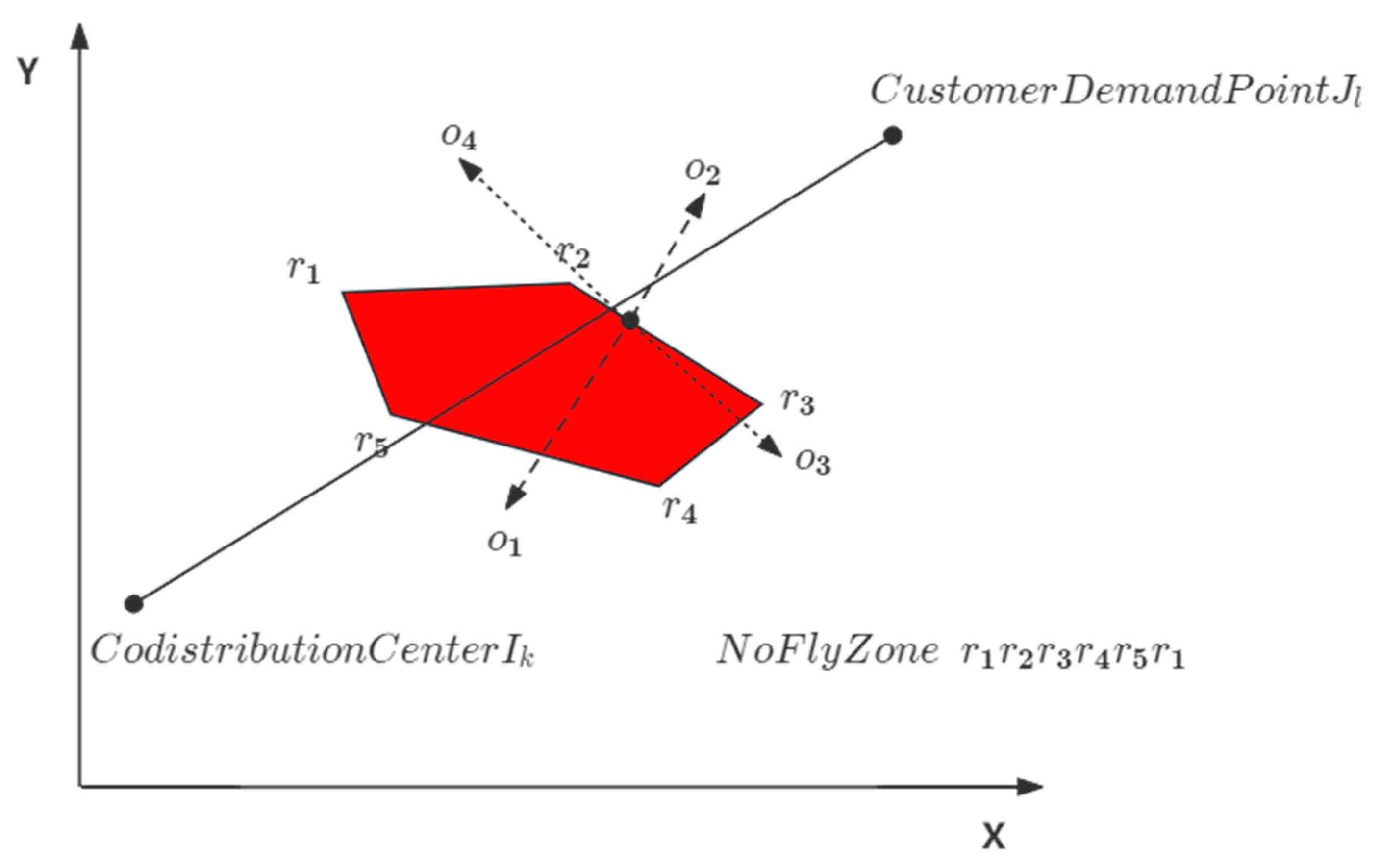
4.2.5. No-Fly-Zone Handling

The no-fly zone can be regarded as a set of vertices surrounded by a closed graph of multiple line segments. To determine whether the delivery path of the UAV crosses the no-fly zone, we can calculate the number of directions of the line segments and check whether the straight line connecting the co-distribution center and the customer demand point intersects with the boundary line segments of the no-fly zone.

As shown in Figure 3, for co-distribution center $I_k\left(x_{l_k},y_{l_k}\right)$ and customer demand point $J_l\left(x_{J_l},y_{J_l}\right)$, when determining whether their connecting lines pass through any polygon of the no-fly zone, $\overrightarrow{R}=\left[r_0(x_{r_0},y_{r_0}),r_1(x_{r_1},y_{r_1}),\cdots ,r_n(x_{r_n},y_{r_n})\right],n\ge 2$, can be transformed into the problem of determining whether the connecting lines intersect with the sides of the polygon. This can be carried out using the number of directions.

For any line segment in the no-fly zone, calculate the following four directions:

$$\left\{\begin{array}{l}{o}_1=\overrightarrow{(I_k-r_q)}\times \overrightarrow{(r_{q+1}-r_q)}\\ o_2=\overrightarrow{(J_l-r_q)}\times \overrightarrow{(r_{q+1}-r_q)}\\ o_3=\overrightarrow{(r_q-J_l)}\times \overrightarrow{(I_k-J_l)}\\ o_4=\overrightarrow{(r_{q+1}-J_l)}\times \overrightarrow{(I_k-J_l)}\end{array}\right.$$

(28)

The product of the number of directions has the following cases:

$$\left\{\begin{array}{l}{o}_1\times o_2<0and{o}_3\times o_4<0,\mathrm{intersecting}\\ o_1\times o_2>0and{o}_3\times o_4>0,\mathrm{not}\mathrm{intersecting}\\ o_1\times o_2=0and{o}_3\times o_4=0,\mathrm{patallel}\mathrm{or}\mathrm{intersecting}\mathrm{endpoints}\end{array}\right.$$

(29)

In Equation (29), if the product of the number of directions is 0, then the two segments share the same line, or the endpoint of one line segment is on the line where the other line segment is located. At this point, we can determine whether the bounding boxes of line segments $\overrightarrow{r_q{r}_{q+1}}$ and $\overrightarrow{I_k{J}_l}$ overlap on the x- and y-axes using Equations (30) and (31). If these equations are simultaneously satisfied, then the two line segments are partially overlapping, i.e., they intersect.

$$\max (\min (r_q(x),r_{q+1}(x)),\min (I_k(x),J_l(x)))\le \min (\max (r_q(x),r_{q+1}(x)),\max (I_k(x),J_l(x)))$$

(30)

$$\max (\min (r_q(y),r_{q+1}(y)),\min (I_k(y),J_l(y)))\le \min (\max (r_q(y),r_{q+1}(y)),\max (I_k(y),J_l(y)))$$

(31)

5. Analysis

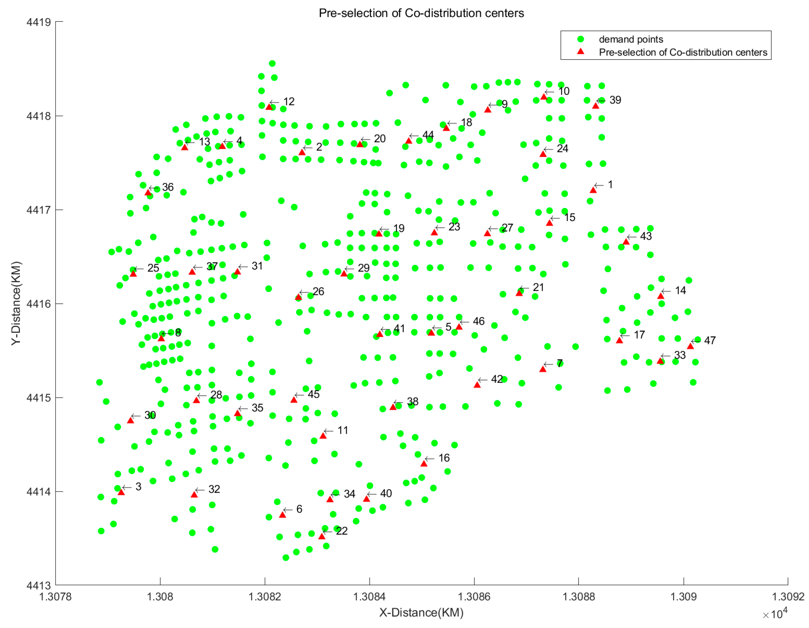
5.1. Preselected Set Construction

To verify the feasibility of the proposed algorithm, we considered the Wangsheren area of Jinan City, China, as an example. Using the public control plan data on the Jinan Natural Resources and Planning Bureau website, as well as an electronic network map and the actual logistics and distribution demand, 492 customer demand points were identified. According to the land use nature of the different parcels and planning indicators, such as the plot ratio, the distribution of each demand point was calculated. The demand corresponding to the first 100 points is listed in

Table 3. First 100 points and demands of the region.

Point	Demand	Point	Demand	Point	Demand	Point	Demand	Point	Demand
1	278	21	584	41	1218	61	1529	81	1047
2	541	22	152	42	324	62	445	82	1044
3	358	23	229	43	404	63	254	83	669
4	494	24	327	44	348	64	1333	84	1450
5	222	25	697	45	578	65	319	85	518
6	187	26	195	46	194	66	842	86	746
7	495	27	1417	47	636	67	1058	87	725
8	179	28	885	48	1062	68	222	88	1574
9	387	29	1206	49	2860	69	910	89	844
10	846	30	1180	50	2394	70	729	90	1305
11	1072	31	401	51	749	71	722	91	727
12	892	32	658	52	1075	72	1232	92	852
13	476	33	353	53	451	73	529	93	1316
14	581	34	518	54	721	74	312	94	483
15	137	35	338	55	746	75	291	95	449
16	624	36	195	56	868	76	668	96	526
17	2787	37	961	57	1695	77	548	97	1645
18	292	38	231	58	1175	78	663	98	287
19	874	39	293	59	433	79	942	99	327
20	634	40	411	60	3276	80	444	100	567

. The distribution of demand points is illustrated in Figure 4.

According to Table 3, Total Demand = 303,752 and Average Demand = 617.38. Before starting the clustering operation, a Cartesian coordinate transformation was applied to the latitude and longitude coordinates of the original data using the Mercator projection method. Let the radius of the earth be r, the longitude be l_o, and the latitude be la. Therefore, the Cartesian XY coordinates can be expressed as

$$\left\{\begin{array}{l}X=l_o\cdot R\\ Y=R\cdot \ln \left[\tan \left(\frac{\pi }{4}+\frac{la}{2}\right)\right]\end{array}\right.$$

(32)

The service radius of the co-distribution center, R, took the value $\left[0.7,0.8,0.9,1.0,1.1,1.2,1.3\right]\mathrm{k}\mathrm{m}$. The values of K considered here were $[14,16,19,23,29,36,47]$. K-means clustering analysis using Matlab was performed, and compactness (CP), separation (SP), the Davies–Bouldin index (DBI), and the Dunn validity index (DVI) were calculated for each value of K [27]. The K-means clustering results are presented in

Table 4. Comparison of metrics for clustering results.

K	CP	SP	DB	DVI
14	27.4086	1.1806	0.7883	0.0631
16	24.2683	1.1166	0.8294	0.0647
19	7.2490	1.0756	0.8364	0.0545
23	9.6046	0.8206	0.8656	0.0701
29	12.6379	0.7496	0.8308	0.0772
36	6.0788	0.5983	0.8823	0.0711
47	1.2362	0.4249	0.8446	0.1018

.

The CP and DVI values were optimized when the number of clusters was 47. From the perspective of the solution space, a higher number of co-distribution centers in the preselected set gave a higher-dimensional solution space, making it easier to explore better solutions using the optimization algorithm. Thus, it was reasonable to set the number of co-distribution centers to 47. The relationship between the co-distribution centers and demand points is shown in Figure 5.

From Figure 5, it is clear that the alternative set of distribution centers is uniformly distributed inside the demand points. The distribution trend indicates that the preselected set is largely within the region with dense demand points and away from the region with sparse demand points, which is in line with expectations. In the next section, the distribution center location problem was solved based on this preselected set.

5.2. Model Parameters

According to field research on urban end distribution, around 50% of regular orders weigh 2–5 kg. Combined with the technical performance parameters of common logistics drone models, this paper considered a six-rotor small drone for end distribution. The construction cost of common distribution centers includes the costs of site lease, transformation, and control facilities; the distribution cost includes the costs of the acquisition of transportation tools, energy consumption, personnel, and other expenditures. The business scope of terminal outlets includes downstream dispatching and upstream receiving. Therefore, upstream and downstream business volume research statistics were used to determine the downstream distribution cost of a single item. The model parameter settings are presented in

Table 5. Comparison of metrics for clustering results.

Parameter	Meaning	Initial Value	Parameter	Meaning	Initial Value
Es1	UAV co-distribution center capacity	10,000	Qu	Maximum load capacity of the UAV (kg)	20
Es2	Vehicle co-distribution center capacity	15,000	Qk	Maximum load capacity of the vehicle (kg)	200
Du	Maximum range of the UAV (km)	20	Dk	Maximum range of the vehicle (km)	50
tu	Average delivery speed of the UAV (km/h)	20	tk	Average delivery speed of the vehicle (km/h)	10
C1	Construction cost of the UAV co-distribution center (104 CNY)	12	C2	Construction cost of the vehicle co-distribution center (104 CNY)	7
Cut1	Unit distribution cost of UAVs (CNY/pc)	0.84	Ckt2	Unit distribution cost of vehicles (CNY/pc)	0.62
MaxIteration	Maximum number of iterations of gray wolf optimization	500	N	Wolf pack size of gray wolf optimization	30

.

To simulate real airspace control, two quadrilateral no-fly zones were set up in the map. Each no-fly zone contained four vertices, which had the following coordinates:

$$\begin{array}{l}NFZ1\_x=[13083.1,13082.8,13083.2,13083.7,13083.1]\\ NFZ1\_y=[4417.33,4417.03,4416.83,4417.17,4417.33]\\ NFZ2\_x=[13083.4,13083.0,13083.3,13083.7,13083.4]\\ NFZ2\_y=[4415.68,4415.39,4415.03,4415.43,4415.69]\end{array}$$

(33)

5.3. Solution Results of GWO

The parameter values listed in Section 4.2 were substituted into the GWO site selection model. After the iterative operation was completed, 28 of the 47 points in the preselected set of co-distribution centers were chosen for co-distribution centers. Among them, 15 were air co-distribution centers and 13 were ground co-distribution centers. The correspondence and specific structure of the co-distribution centers and demand points are listed in

Table 6. Comparison of metrics for clustering results.

Number of Selected Points	Type of Co-Distribution Center	Corresponding Set of Demand Points
2	Vehicle	12, 14, 24, 28, 32, 37, 39, 40, 41, 43, 45, 55, 62, 63, 65, 70, 71, 72, 75, 76, 78, 83, 94, 95
3	Vehicle	102, 108, 111, 127, 145, 183, 209, 212, 218, 221, 223, 225, 226, 243, 265, 268, 348
4	Vehicle	279, 280, 301, 302, 327, 328, 329, 331, 334, 346, 367, 368
7	Vehicle	378, 397, 398, 399, 413, 419, 427, 430, 455, 456, 466, 467, 468, 472, 473, 482, 484, 486, 488, 489
8	UAV	320, 343, 349, 360, 365, 369, 370, 371, 373, 377, 380, 402, 405, 415, 438
9	Vehicle	89, 101, 116, 117, 128, 137, 154, 162
10	Vehicle	113, 140, 141, 142, 170, 171, 172, 204, 219, 229, 257, 263, 264, 304, 335
14	UAV	107, 135, 184, 199, 205, 210, 238, 250, 255, 256, 267, 285, 287, 288, 289, 298, 311
15	UAV	342, 355, 374, 375, 376, 379, 382, 388, 391, 406, 409, 410, 411, 425, 428, 432, 433, 434, 435, 445, 451, 453, 454, 459
16	UAV	251, 254, 261, 266, 269, 286, 290, 291, 297, 299, 300, 308, 309, 310, 325, 336, 339, 340
17	UAV	259, 270, 271, 292, 293, 313, 317, 318, 322, 323, 341, 351, 352, 354, 358
18	UAV	67, 86, 88, 91, 93, 114, 118, 120, 121, 146, 147, 163, 196
19	Vehicle	400, 401, 431, 457, 458, 469, 470, 477, 479
20	UAV	149, 173, 174, 175, 190, 191, 192, 230, 233, 234, 235, 236
22	UAV	364, 394, 395, 396, 408, 418, 422, 423, 429, 440, 442, 443, 446, 449, 463, 464, 465, 475, 490, 491, 492
24	UAV	103, 104, 106, 119, 122, 125, 129, 130, 132, 134, 136, 138, 148, 153, 156, 157, 159, 161, 165, 166, 167, 169, 179, 186, 188, 189, 201, 213, 214, 216, 217, 239, 241, 246, 248, 258, 260
25	UAV	252, 253, 262, 272, 273, 274, 281, 294, 295, 296, 315, 316, 319, 321, 324, 347, 353
26	UAV	98, 99, 109, 115, 126, 131, 133, 164, 180, 187, 198, 203, 206, 207, 220, 222, 231, 237, 249
27	UAV	22, 25, 26, 33, 34, 35, 36, 38, 51, 59, 64, 66, 68, 69, 90, 92
28	Vehicle	1, 2, 4, 5, 6, 7, 9, 10, 11, 13, 15, 18, 20, 21, 27, 29, 30, 31, 42, 50, 87
29	Vehicle	105, 110, 112, 139, 144, 155, 160, 168, 185, 200, 202, 215, 224, 242, 247, 303
30	Vehicle	3, 8, 16, 17, 19, 23, 44, 46, 47, 48, 52, 53, 54, 56, 73, 80, 81, 82, 96
31	UAV	361, 362, 363, 381, 383, 384, 386, 387, 390, 392, 393, 407, 414, 416, 417, 420, 421, 444, 447, 448, 450, 452, 460, 478, 481
33	Vehicle	49, 57, 58, 60, 61, 74, 77, 79, 84, 85, 100
36	Vehicle	158, 181, 208, 211, 240, 244, 276, 277, 278, 306, 307, 332, 333, 344, 345, 366
38	UAV	385, 389, 403, 404, 412, 424, 426, 436, 437, 439, 441, 461, 462, 471, 474, 476, 480, 483, 485, 487
43	Vehicle	97, 123, 124, 143, 150, 151, 152, 176, 177, 178, 182, 193, 194, 195, 227, 228, 232, 282, 284, 314
47	UAV	197, 245, 275, 283, 305, 312, 326, 330, 337, 338, 350, 356, 357, 359, 372

.

The final fitness value of the optimal solution was 0.1334, corresponding to a total time cost of 18.1012 h and a total economic cost of CNY 82,501,686. The co-distribution center site selection and demand point correspondence is shown in Figure 6.

5.4. Comparison of Algorithm Performance

To further verify the exploration ability and optimality of the GWO algorithm, the results were compared with those given by particle swarm optimization (PSO). PSO is a swarm heuristic algorithm that simulates the flocking behavior of birds and searches for an optimal solution through collaboration and information sharing among particles in the flock [28]. The convergence speeds of the GWO and PSO algorithms are shown in Figure 7.

The global information-sharing mechanism of PSO ensures a rapid initial convergence speed, but after a certain number of iterations, the algorithm becomes stuck around a locally optimal solution and its fitness remains unchanged. The social hierarchical structure and the group-hunting mechanism of GWO ensure a strong exploration ability, allowing it to continue moving toward a globally optimal solution. The adaptability of GWO decreases as the number of iterations increases, until adaptability stabilizes. The fitness of the optimal solution is improved by about 34.1% compared with that of PSO. The figure also shows that the gray wolf algorithm performs better than the particle swarm algorithm in terms of global exploration ability. By dynamically adjusting the position of the leader wolf and the position of other individuals, it can effectively balance exploration and exploitation and reduce the possibility of premature convergence.

In its implementation, the gray wolf algorithm needs to set only the size of the population and the number of iterations, without the need for a large number of parameters to be set and tuned, and the implementation is relatively simple. However, the particle swarm algorithm needs to adjust a number of parameters, such as inertia weights, learning factors, and speed range, and its operation speed and convergence speed are greatly affected by the impact of a single parameter; in addition, it is more unstable, which affects the overall efficiency of the algorithm.

5.5. Operational Effectiveness of the Air–Ground Cooperative Co-Distribution Network

To verify the validity and implementation of the model, the results were compared against those for a traditional distribution network with the same distribution demand. According to a field survey of the distribution network layout and operation in Wangsheren, about 70–80 distribution networks complete 300,000 daily deliveries. The cost mainly includes the costs of the construction or leasing of the network, labor, and vehicle purchase and use. The average distribution cost is CNY 0.5–0.6, and the average time for the network to complete the daily distribution is about 4 h. According to the calculation results of the proposed model in Section 5.3, the number of open-space cooperative terminal co-distribution centers is much lower than the number of traditional terminal points, which effectively improves the land intensification and urban spatial environment quality. In terms of cost and delivery time, the parameter settings in this paper mainly consider the current level of UAV equipment and market price. Restricted by existing problems, such as limited endurance, load capacity, and battery loss, UAV co-distribution centers have a relatively high cost, and the single-delivery cost calculated by the model is 35–50% higher than that of traditional terminal distribution. However, the average time required for co-distribution centers to complete all deliveries is only 15–20% of that for traditional terminal outlets, indicating a significant improvement in the efficiency of terminal distribution and customer satisfaction. The main source of profit for distribution enterprises is higher-value-added services, such as upward receipt. Therefore, reduced delivery times greatly improve the service capability of this part of the business. Increasing the comprehensive income of distribution enterprises is of great significance. With improvements in the technical level of UAVs, the associated distribution costs will gradually decrease, and the labor cost of vehicle-sharing centers will be greatly increased.

6. Conclusions

Based on the concept of co-distribution, this paper studied the layout and site selection problem of urban terminal co-distribution centers with UAV and vehicle co-distribution. We established a planning model to minimize the network operation cost and distribution time and designed a GWO algorithm based on K-means clustering to solve the optimization problem. The model and algorithm were tested using actual data from the Wangsheren area of Jinan City, China, and the results were compared with those given by PSO. The comparison results showed that GWO is highly effective for solving this type of siting problem, and the fitness value of the GWO is reduced by 34.1%. The collaborative layout scheme of air and ground co-distribution centers constructed in this paper produced significant improvements in distribution efficiency, thus improving the urban environment and ground transportation operation quality, optimizing the distribution enterprise revenue structure, and enhancing the comprehensive benefits of terminal distribution. In future work, we will consider the special distribution characteristics of different functional groups in the city and refine the applicable scenarios and constraints of drone and vehicle distribution. Additionally, we will attempt to improve the end distribution network.

References

1. Available online: http://www.caac.gov.cn/HDJL/YJZJ/202208/P020220822615871900321.pdf (accessed on 1 June 2024).
2. Özmen, M.; Aydoğan, E.K. Robust multi-criteria decision making methodology for real life logistics center location problem. Artif. Intell. Rev. 2020, 53, 725–751. [Google Scholar] [CrossRef]
3. Mousavi, S.M.; Antuchevičienė, J.; Zavadskas, E.K.; Vahdani, B.; Hashemi, H. A new decision model for cross-docking center location in logistics networks under interval-valued intuitionistic fuzzy uncertainty. Transport 2019, 34, 30–40. [Google Scholar] [CrossRef]
4. Ji, Y.; Bei, B.; Chu, H.; Cheng, F. Optimization research of terminal distribution network of express enterprise based on two-stage algorithm. Syst. Eng. 2019, 37, 100–105. [Google Scholar]
5. Cui, D. Research on the Construction of the Terminal Common Distribution Network of Express Delivery Enterprises. Master’s Thesis, Beijing Jiaotong University, Beijing, China, 2019. [Google Scholar]
6. Bi, K. Research on Location of Collaborative Distribution Service Station for Urban Terminal Express Delivery Based on Crowdsourcing. Master’s Thesis, Beijing University of Posts and Telecommunications, Beijing, China, 2021. [Google Scholar]
7. Shavarani, S.M.; Nejad, M.G.; Rismanchian, F.; Izbirak, G. Application of hierarchical facility location problem for optimization of a drone delivery system: A case study of Amazon prime air in the city of San Francisco. Int. J. Adv. Manuf. Technol. 2018, 95, 3141–3153. [Google Scholar] [CrossRef]
8. Venkatesh, N.; Payan, A.P.; Justin, C.Y.; Kee, E.; Mavris, D. Optimal siting of sub-urban air mobility (suam) ground architectures using network flow formulation. In Proceedings of the AIAA AVIATION 2020 FORUM, Virtual, 15–19 June 2020; p. 2921. [Google Scholar]
9. German, B.; Daskilewicz, M.; Hamilton, T.K.; Warren, M.M. Cargo delivery by passenger EVTOL aircraft: A case study in the San Francisco bay area. In Proceedings of the AIAA Aerospace Sciences Meeting, San Francisco, CA, USA, 8 January 2018. [Google Scholar]
10. Ren, X.; Wang, L.; Wang, J. Automatic Vertiport Location of Unmanned Aerial Vehicle Based on Partition Optimization. Oper. Res. Manag. Sci. 2023, 32, 20–26. [Google Scholar]
11. Lu, L.; Hu, Z. Island UAV Delivery Relay Station Siting-Path Optimization. J. Dalian Univ. Technol. 2022, 62, 299–306. [Google Scholar]
12. Qian, X.; Zhang, H.; Zhang, F. Research on site selection and allocation of landing sites for end-of-line distribution logistics UAVs. J. Wuhan Univ. Technol. (Transp. Sci. Eng.) 2021, 45, 682–693. [Google Scholar]
13. Feng, D. Research on the Layout Planning Method of Urban Logistics UAV Vertiports. Master’s Thesis, Nanjing University of Aeronautics and Astronautics, Nanjing, China, 2022. [Google Scholar]
14. Borghetti, F.; Caballini, C.; Carboni, A.; Grossato, G.; Maja, R.; Barabino, B. The use of drones for last-mile delivery: A numerical case study in Milan, Italy. Sustainability 2022, 14, 1766. [Google Scholar] [CrossRef]
15. Sharma, I.; Kumar, V.; Sharma, S. A comprehensive survey on grey wolf optimization. Recent Adv. Comput. Sci. Commun. (Former. Recent Pat. Comput. Sci.) 2022, 15, 323–333. [Google Scholar]
16. Kumar, A.; Pant, S.; Ram, M. Gray wolf optimizer approach to the reliability-cost optimization of residual heat removal system of a nuclear power plant safety system. Qual. Reliab. Eng. Int. 2019, 35, 2228–2239. [Google Scholar] [CrossRef]
17. El Gayyar, M.; Emary, E.; Sweilam, N.H.; Abdelazeem, M. A hybrid Grey Wolf-bat algorithm for global optimization. In Proceedings of the International Conference on Advanced Machine Learning Technologies and Applications, Cairo, Egypt, 22–24 February 2018; Springer: Cham, Switzerland, 2018; pp. 3–12. [Google Scholar]
18. Fouad, M.M.; Hafez, A.I.; Hassanien, A.E.; Vaclav, S. Grey wolves optimizer-based localization approach in WSNs. In Proceedings of the 2015 11th International Computer Engineering Conference (ICENCO), Cairo, Egypt, 29–30 December 2015; pp. 256–260. [Google Scholar]
19. Long, W.; Wu, T.; Cai, S.; Liang, X.; Jiao, J.; Xu, M. A novel grey wolf optimizer algorithm with refraction learning. IEEE Access 2019, 7, 57805–57819. [Google Scholar] [CrossRef]
20. Mittal, N.; Singh, U.; Sohi, B.S. Modified grey wolf optimizer for global engineering optimization. Appl. Comput. Intell. Soft Comput. 2016, 2016, 7950348. [Google Scholar] [CrossRef]
21. Zhang, S.; Zhou, Y.; Li, Z.; Pan, W. Grey wolf optimizer for unmanned combat aerial vehicle path planning. Adv. Eng. Softw. 2016, 99, 121–136. [Google Scholar] [CrossRef]
22. Sujatha, K.; Shalini Punithavathani, D. Optimized ensemble decision-based multi-focus imagefusion using binary genetic Grey-Wolf optimizer in camera sensor networks. Multimed. Tools Appl. 2018, 77, 1735–1759. [Google Scholar] [CrossRef]
23. King, L.J. Central Place Theory; West Virginia University: Morgantown, WV, USA, 2020. [Google Scholar]
24. Su, W. Research on the Layout Planning of Express Terminal Joint Distribution Network. Master’s Thesis, Beijing Jiaotong University, Beijing, China, 2024. [Google Scholar]
25. Ahmed, M.; Seraj, R.; Islam, S.M.S. The k-means algorithm: A comprehensive survey and performance evaluation. Electronics 2020, 9, 1295. [Google Scholar] [CrossRef]
26. Mirjalili, S.; Mirjalili, S.M.; Lewis, A. Grey wolf optimizer. Adv. Eng. Softw. 2014, 69, 46–61. [Google Scholar] [CrossRef]
27. Nagargoje, A.; Kankar, P.K.; Jain, P.K.; Tandon, P. Performance evaluation of the data clustering techniques and cluster validity indices for efficient toolpath development for incremental sheet forming. J. Comput. Inf. Sci. Eng. 2021, 21, 031001. [Google Scholar] [CrossRef]
28. Jain, M.; Saihjpal, V.; Singh, N.; Singh, S.B. An overview of variants and advancements of PSO algorithm. Appl. Sci. 2022, 12, 8392. [Google Scholar] [CrossRef]
Figure 1. Schematic diagram of the planning layout of air–ground cooperative co-distribution centers.
Applsci 14 05814 g001
Figure 2. Flowchart of the site selection method based on GWO.
Applsci 14 05814 g002
Figure 3. No-fly-zone-crossing judgment method based on direction number.
Applsci 14 05814 g003
Figure 4. Distribution of demand points.
Applsci 14 05814 g004
Figure 5. Clustering results for the preselected set of co-distribution centers.
Applsci 14 05814 g005
Figure 6. Results of site selection for the co-distribution centers.
Applsci 14 05814 g006
Figure 7. Convergence speeds of the GWO and PSO algorithms.
Applsci 14 05814 g007