

Early Detection and Stability Assessment of Hazardous Rock Masses in Steep Slopes


Abstract
1. Introduction
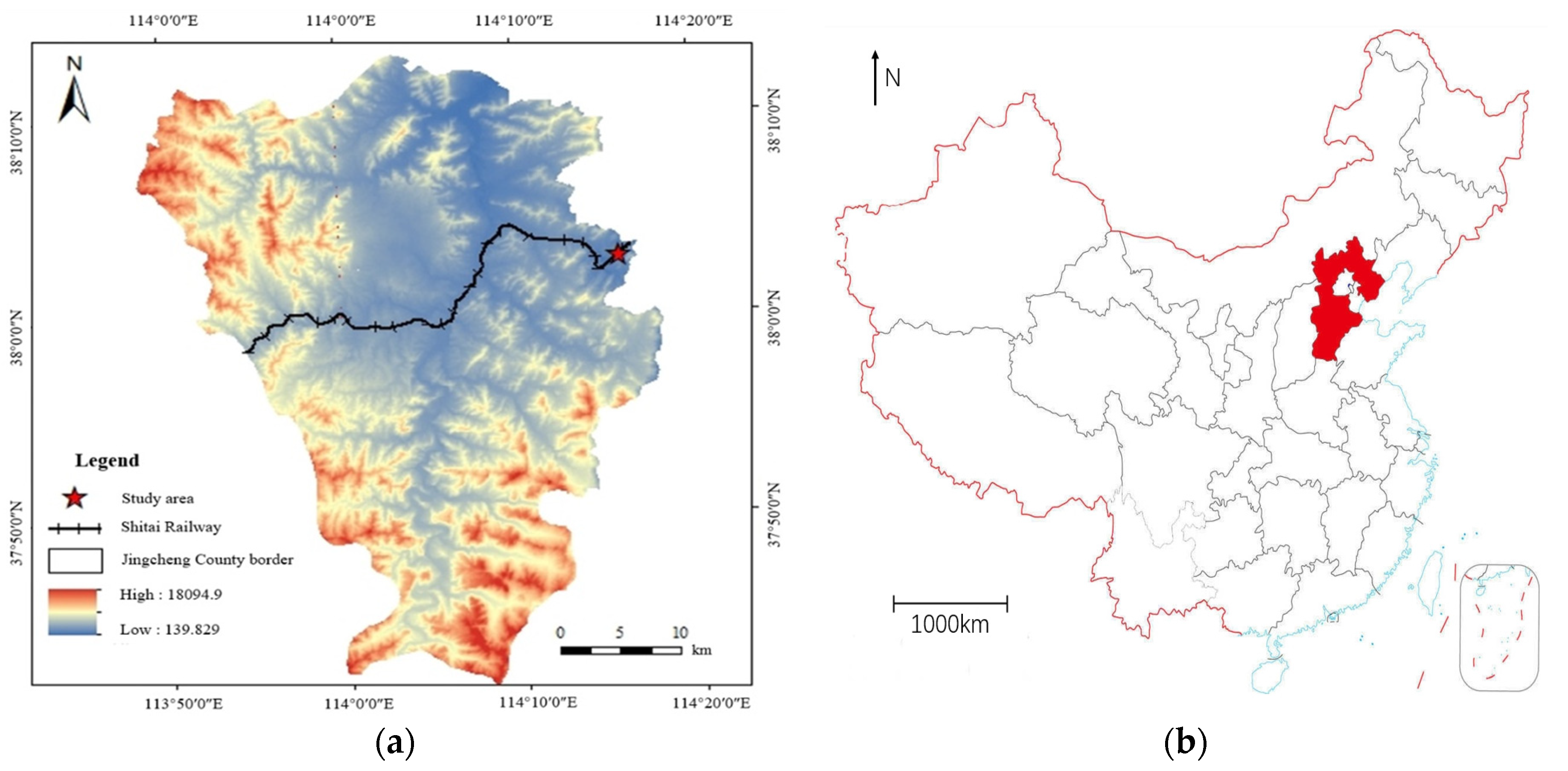
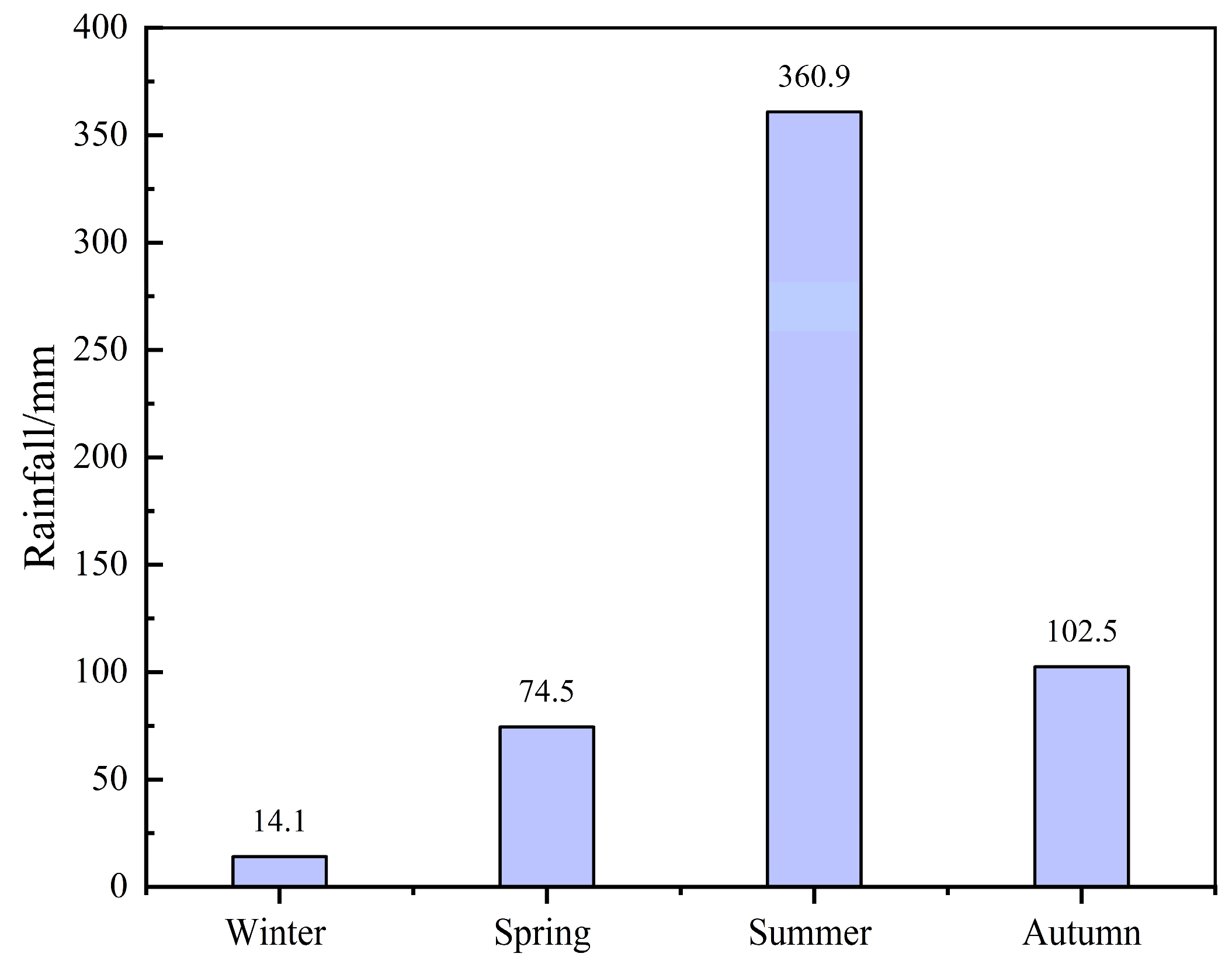
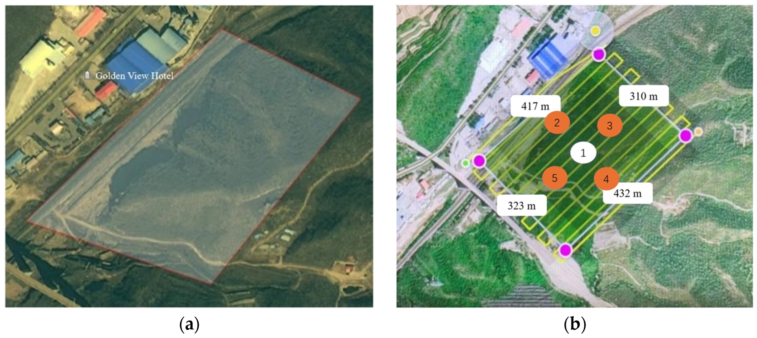
2. Brief Report on Engineering Background and Geological Setting
3. Method
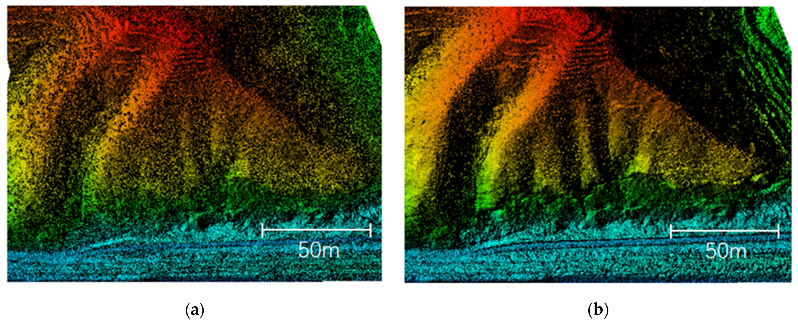
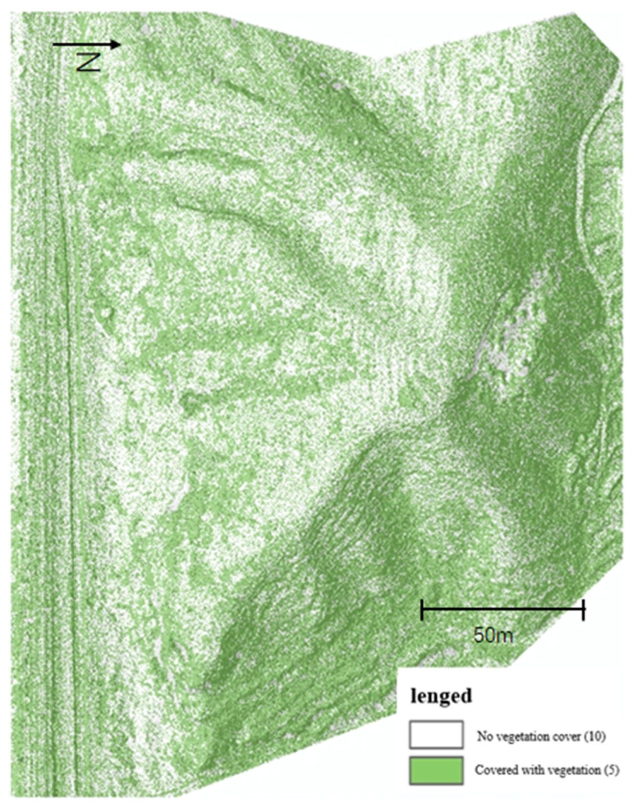
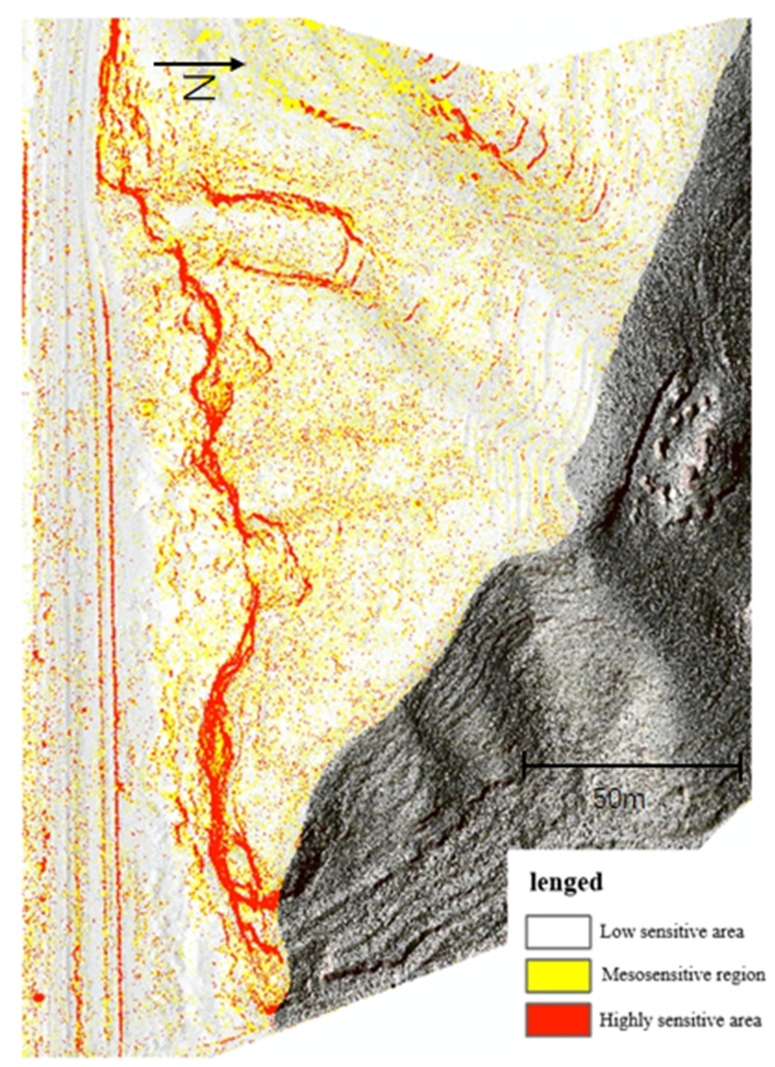
3.1. Processing of Aerial Survey Image Data
3.2. Early Identification Model of Dangerous Rock Mass
3.3. Stability Evaluation Index System and Weight Analysis
4. Results and Discussion
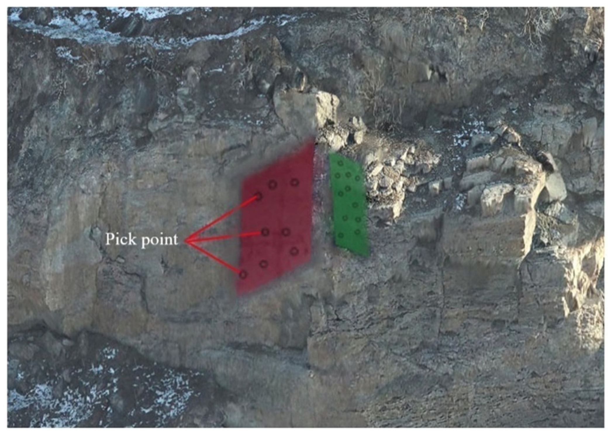
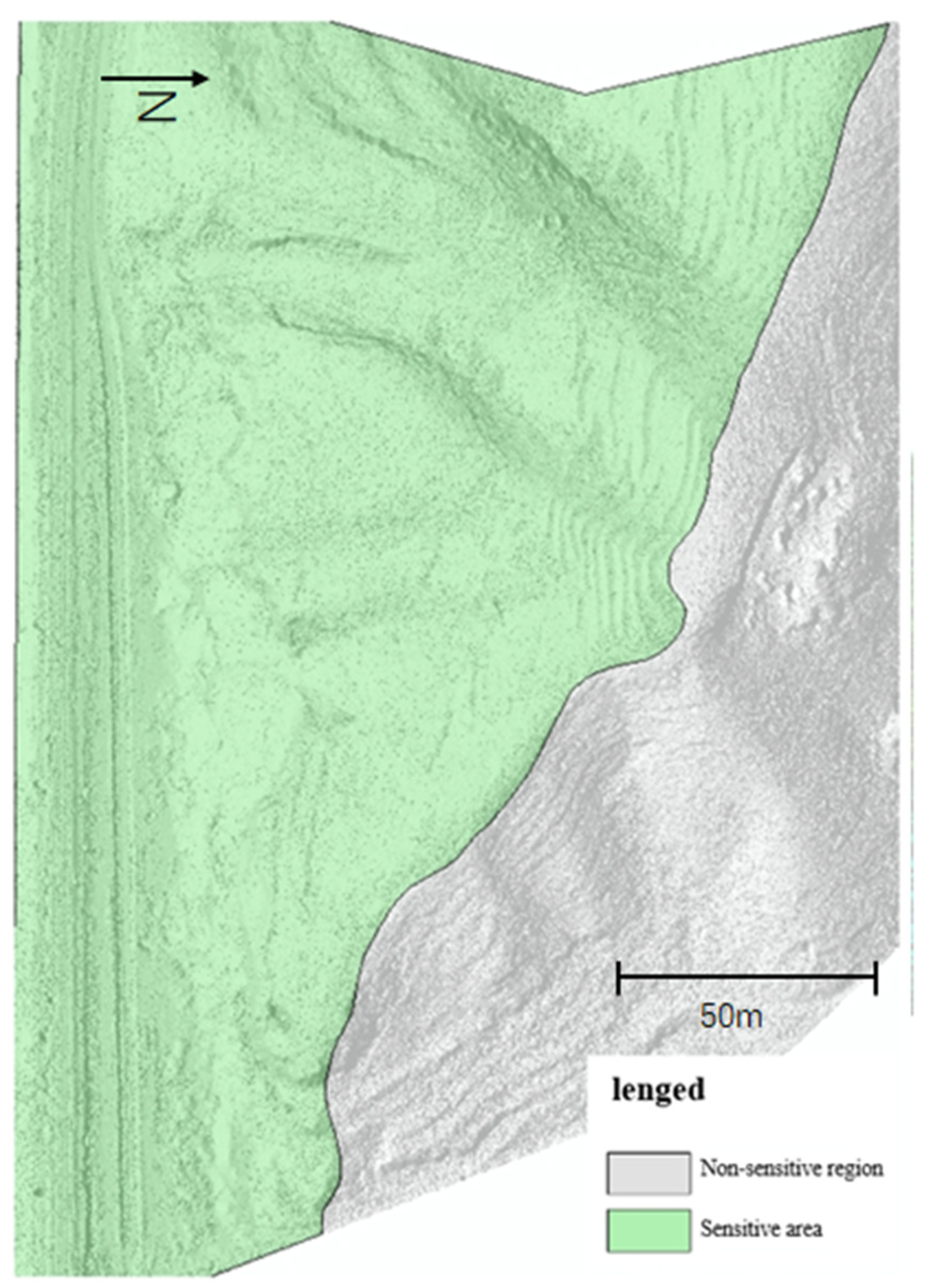
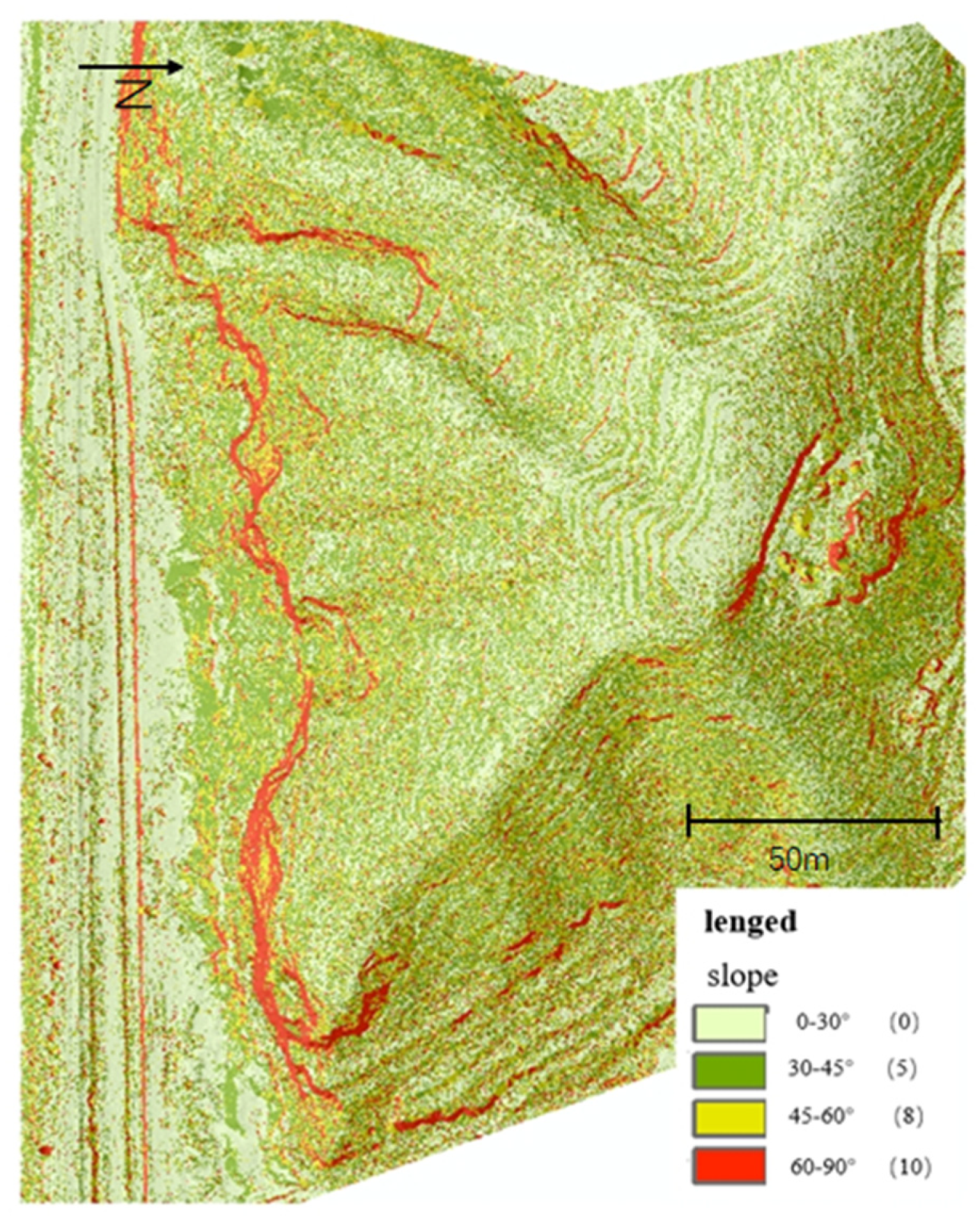
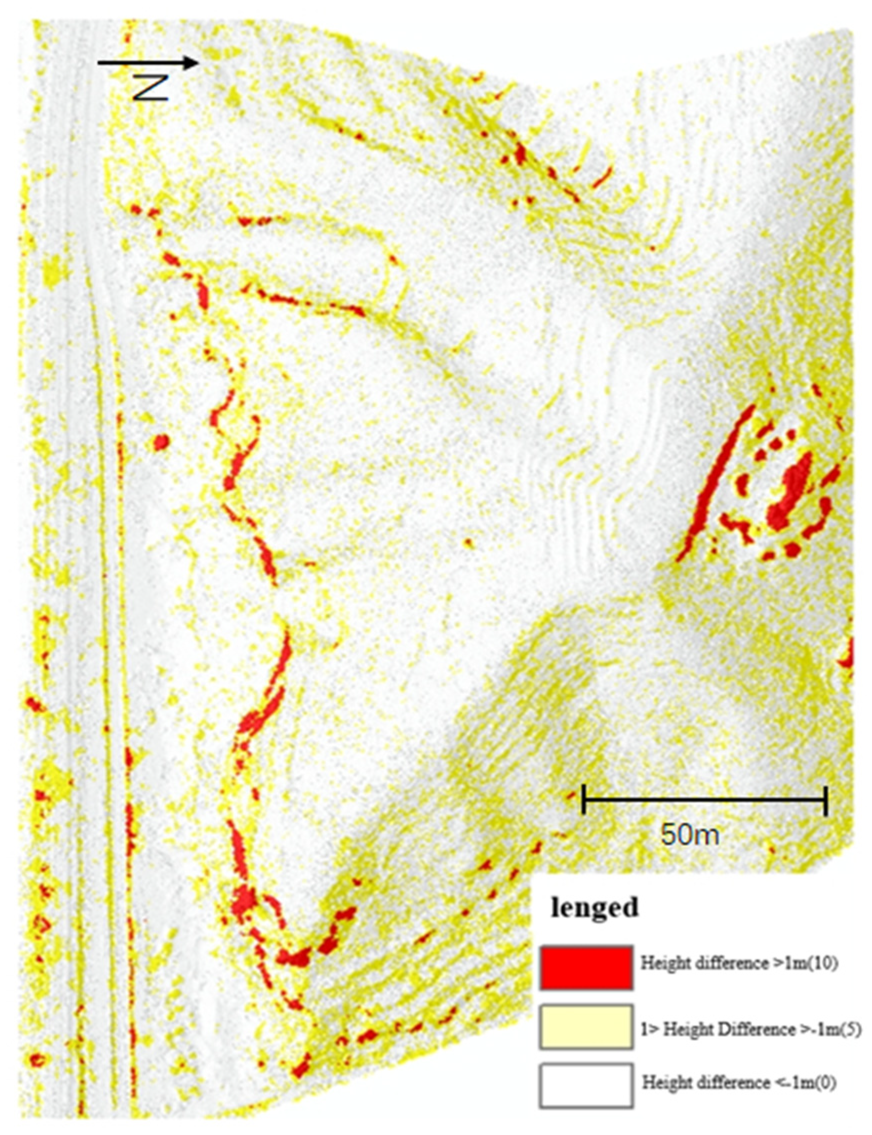
4.1. Early Identification Results of Dangerous Rock Masses
4.2. Stability Evaluation Results and Verification
4.3. Limitations of the Proposed Approach
5. Conclusions
- The UAV photogrammetry technology was utilized to acquire high-resolution remote sensing images, a three-dimensional point-cloud model, and other data results. The topographic conditions of the slope were extracted and superimposed through the geographic information system in order to identify potential dangerous rock areas and generate a map of hazardous rock zones.
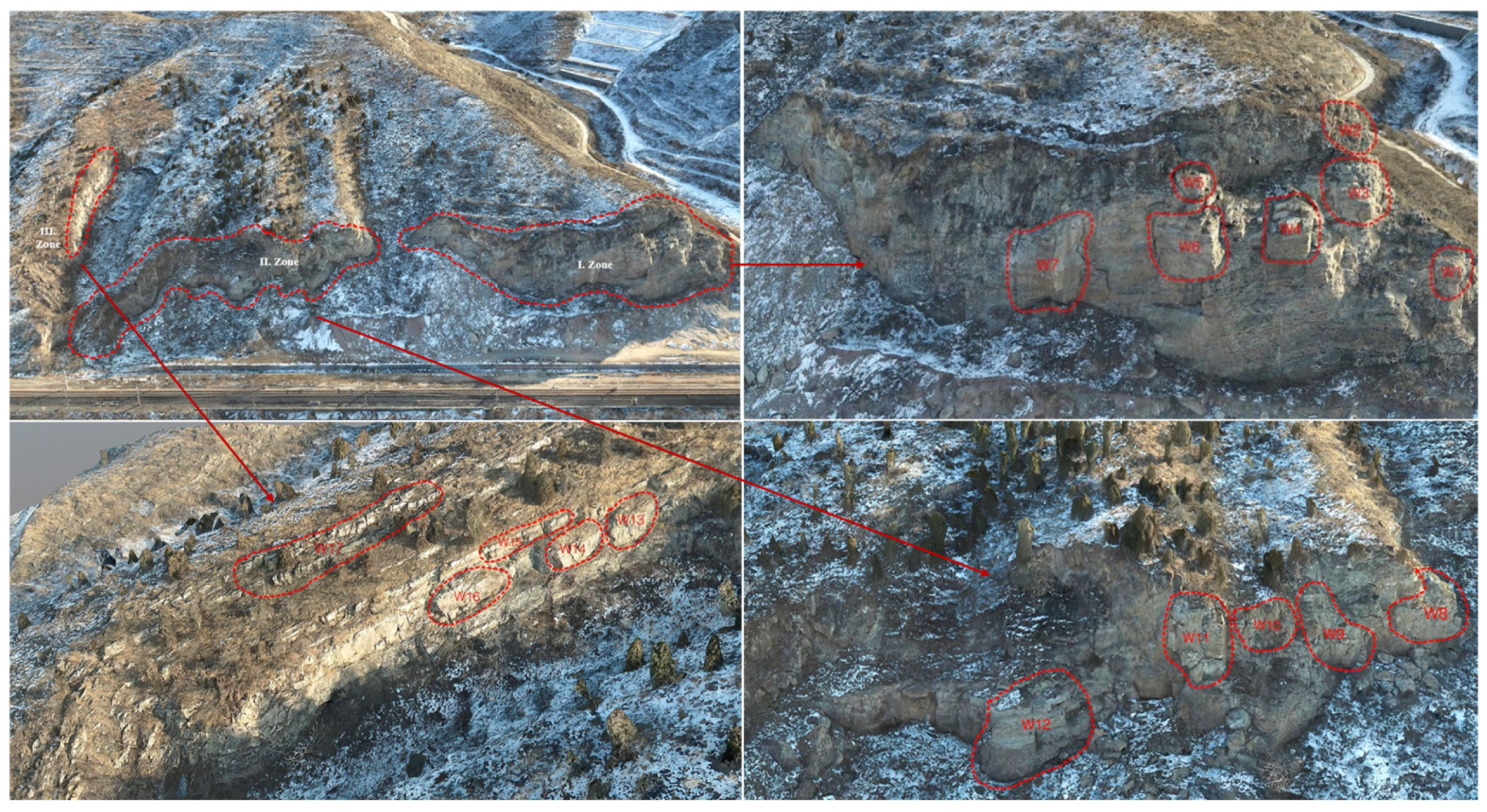
- Based on the three-dimensional model, a detailed investigation was conducted into the development characteristics and instability mode of the hazardous rocks. The distribution and development characteristics of the hazardous rock mass were categorized into three dangerous rock belts, with consensus identifying 17 hazardous rock masses. These masses were primarily distributed within an elevation range of 150~200 m, mostly small- to medium-sized in scale.
- An evaluation index system for assessing the stability of hazardous rock masses has been established, with nine influencing factors selected as stability evaluation indices. The weights of these indices have been determined using analytic hierarchy process. Evaluation results indicate that W4, W6, and W10 rocks in the study area are unstable, accounting for 17.6% based on verification by applying the limit equilibrium principle.
Author Contributions
Funding
Institutional Review Board Statement
Informed Consent Statement
Data Availability Statement
Conflicts of Interest
References
- Chen, H.; Wang, R.; Tang, H. Review on research status and trend of dangerous rock. J. Chongqing Jiaotong Univ. (Nat. Sci. Ed.) 2003, 22, 18–22. [Google Scholar]
- Jia, Y.; Li, Z.; Jiang, T.; Li, Y.; Wang, S.; Song, G. Study on Early Identification of Landslide Perilous Rocks Based on Multi-Dynamics Parameters. Sustainability 2023, 15, 6296. [Google Scholar] [CrossRef]
- Hu, H. Collapse and Falling Rock; China Railway Publishing House: Beijing, China, 1989. [Google Scholar]
- Du, Y.; Xie, M. Indirect method for the quantitative identification of unstable rock. Nat. Hazards 2022, 112, 1005–1012. [Google Scholar] [CrossRef]
- Jia, Y.; Song, G.; Wang, L.; Jiang, T.; Zhao, J.; Li, Z. Research on Stability Evaluation of Perilous Rock on Soil Slope Based on Natural Vibration Frequency. Appl. Sci. 2023, 13, 2406. [Google Scholar] [CrossRef]
- Perrotti, M.; Godone, D.; Allasia, P.; Baldo, M.; Fazio, N.L.; Lollino, P. Investigating the susceptibility to failure of a rock cliff by integrating Structure-from-Motion analysis and 3D geomechanical modelling. Remote Sens. 2020, 12, 3994. [Google Scholar] [CrossRef]
- Emil, B.; Manfred, B.; Martin, K. Radar Remote Sensing to Supplement Pipeline Surveillance Programs through Measurements of Surface Deformations and Identification of Geohazard Risks. Remote Sens. 2020, 12, 3934. [Google Scholar] [CrossRef]
- Guo, C.; Xu, Q.; Dong, X.; Li, W.; Zhao, K.; Lu, H.; Ju, Y. Geohazard Recognition and Inventory Mapping Using Airborne LiDAR Data in Complex Mountainous Areas. J. Earth Sci. 2021, 32, 1079–1091. [Google Scholar] [CrossRef]
- Zhang, Z.; Duan, P.; Li, J.; Chen, D.; Peng, K.; Fan, C. A time-series InSAR processing chain for wide-area geohazard identification. Nat. Hazards 2023, 118, 691–707. [Google Scholar] [CrossRef]
- Kong, D.; Saroglou, C.; Wu, F.; Sha, P.; Li, B. Development and application of UAV-SfM photogrammetry for quantitative characterization of rock mass discontinuities. Int. J. Rock Mech. Min. Sci. 2021, 141, 104729. [Google Scholar] [CrossRef]
- Xu, Q.; Dong, X.; Li, W. Early identification, monitoring and early warning of major geological hazards based on the integration of space-space-earth. J. Wuhan Univ. (Inf. Sci. Ed.) 2019, 44, 957–966. [Google Scholar]
- Menegoni, N.; Giordan, D.; Perotti, C. Reliability and Uncertainties of the Analysis of an Unstable Rock Slope Performed on RPAS Digital Outcrop Models: The Case of the Gallivaggio Landslide (Western Alps, Italy). Remote Sens. 2020, 12, 1635. [Google Scholar] [CrossRef]
- Alvioli, M.; Santangelo, M.; Fiorucci, F.; Cardinali, M.; Marchesini, I.; Reichenbach, P.; Rossi, M.; Guzzetti, F.; Peruccacci, S. Rockfall susceptibility and network-ranked susceptibility along the Italian railway. Eng. Geol. 2021, 293, 106301. [Google Scholar] [CrossRef]
- Damhuis, J.M.R.; Roux, L.P.; Fourie, S.J.C. The identification and mitigation of geohazards using shallow airborne engineering geophysics and land-based geophysics for brown- and greenfield road investigations. Q. J. Eng. Geol. Hydrogeol. 2020, 53, 321–332. [Google Scholar] [CrossRef]
- Albarelli, D.; Mavrouli, O.C.; Nyktas, P. Identification of potential rockfall sources using UAV-derived point cloud. Bull. Eng. Geol. Environ. 2021, 80, 6539–6561. [Google Scholar] [CrossRef]
- Kong, D.; Wu, F.; Saroglou, C. Automatic identification and characterization of discontinuities in rock masses from 3D point clouds. Eng. Geol. 2020, 265, 105442. [Google Scholar] [CrossRef]
- Rodriguez, J.; Macciotta, R.; Hendry, M.T.; Roustaei, M.; Gräpel, C.; Skirrow, R. UAVs for monitoring, investigation, and mitigation design of a rock slope with multiple failure mechanisms—A case study. Landslides 2020, 17, 2027–2040. [Google Scholar] [CrossRef]
- Mancini, F.; Dubbini, M.; Gattelli, M.; Stecchi, F.; Fabbri, S.; Gabbianelli, G. Using unmanned aerial vehicles (UAV) for high-resolution reconstruction of topography: The structure from motion approach on coastal environments. Remote Sens. 2013, 5, 6880–6898. [Google Scholar] [CrossRef]
- Hao, Y.; He, M.; Liu, Y.; Liu, J.; Meng, Z. Range–Visual–Inertial Odometry with Coarse-to-Fine Image Registration Fusion for UAV Localization. Drones 2023, 7, 540. [Google Scholar] [CrossRef]
- Wang, L.; Zhang, J.; Xia, W.; Huang, X.; Tan, G. Dynamic Stability and Fuzzy Reliability Analysis of Toppling Perilous Rock Under Seismic Excitation. J. Earth Sci. 2024, 35, 248–262. [Google Scholar] [CrossRef]
- Peng, H.; Xie, Q.; Chen, B.; Tan, K.; Cao, Z.; Wu, B. Failure mode of the hazardous Diaozui rock mass of the Qutang Gorge in the Three Gorges Reservoir area based on a three-dimensional numerical analysis. Bull. Eng. Geol. Environ. 2024, 83, 100. [Google Scholar] [CrossRef]
- Zuo, R. Evaluation on the Status Quo of Geo-Ecological Environment in Shijiazhuang Area; Hebei University of Geosciences: Shijiazhuang, China, 2016. [Google Scholar]
- Tao, Y.; Xue, Y.; Zhang, Q.; Yang, W.; Li, B.; Zhang, L.; Qu, C.; Zhang, K. Risk Assessment of Unstable Rock Masses on High-Steep Slopes: An Attribute Recognition Model. Soil Mech. Found. Eng. 2021, 58, 175–182. [Google Scholar] [CrossRef]
- Sestras, P.; Bilașco, Ș.; Roșca, S.; Veres, I.; Ilies, N.; Hysa, A.; Spalević, V.; Cîmpeanu, S.M. Multi-Instrumental Approach to Slope Failure Monitoring in a Landslide Susceptible Newly Built-Up Area: Topo-Geodetic Survey, UAV 3D Modelling and Ground-Penetrating Radar. Remote Sens. 2022, 14, 5822. [Google Scholar] [CrossRef]
- Liu, W.L.; Dong, J.X.; Sui, S.G.; Xu, H.H.; Yang, R.X.; Shen, Z.L. Trajectory Analysis and Risk Evaluation of Dangerous Rock Mass Instability of an Overhang Slope, Southwest of China. Adv. Civ. Eng. 2021, 2021, 7153535. [Google Scholar] [CrossRef]
- Liu, W.L.; Dong, J.X.; Sui, S.G.; Xu, H.H.; Yang, R.X.; Shen, Z.L. Stability Assessment of Dangerous Rock Mass of an Overhanging Slope in Puerdu Town, Southwestern China. Adv. Civ. Eng. 2021, 2021, 6526417. [Google Scholar] [CrossRef]
- Mammoliti, E.; Pepi, A.; Fronzi, D.; Morelli, S.; Volatili, T.; Tazioli, A.; Francioni, M. 3D Discrete Fracture Network Modelling from UAV Imagery Coupled with Tracer Tests to Assess Fracture Conductivity in an Unstable Rock Slope: Implications for Rockfall Phenomena. Remote Sens. 2023, 15, 1222. [Google Scholar] [CrossRef]
- Ghorbanzadeh, O.; Meena, S.R.; Blaschke, T.; Aryal, J. UAV-Based Slope Failure Detection Using Deep-Learning Convolutional Neural Networks. Remote Sens. 2019, 11, 2046. [Google Scholar] [CrossRef]
- Zheng, L.; Wu, Y.; Zhu, Z.; Ren, K.; Wei, Q.; Wu, W.; Zhang, H. Investigating the Role of Earthquakes on the Stability of Dangerous Rock Masses and Rockfall Dynamics. Front. Earth Sci. 2022, 9, 824889. [Google Scholar] [CrossRef]
- Zhang, H.; Li, Z.; Chen, G.; Reven, A.; Scharfenberg, B. UAV-based smart rock localization for bridge scour monitoring. J. Civ. Struct. Health Monit. 2021, 11, 301–313. [Google Scholar] [CrossRef]
- Chen, H.; Wang, S.; Chen, J. Theoretical framework of physical evolution of dangerous rock collapse disaster and disaster outbreak time. J. Chongqing Norm. Univ. (Nat. Sci. Ed.) 2020, 37, 121–128. [Google Scholar]
- Wang, M.; Cao, X.; Jia, Q.L. Detailed investigation of dangerous rock mass and 3D scene simulation of collapse process: A case study of high slope of a hydropower station in Southwest China. Chin. J. Geol. Hazards Prev. 2019, 34, 86–96. [Google Scholar]
- Lu, G. Experimental Study on a New Type of Energy Dissipation Reinforced Structure of Sliding Dangerous Rock Mass under Strong Earthquake; Shandong Jianzhu University: Jinan, China, 2023. [Google Scholar]
- Zhang, J.; Wang, L.; Xia, W. Stability reliability calculation of dangerous rock based on fuzzy failure criteria. J. Disaster Prev. Reduct. Eng. 2022, 42, 695–704. [Google Scholar]
- Peng, X.; Wang, Z.; Ma, K. Study on Influence of Slope Blasting Excavation on Stability of Adjacent Dangerous Rock Mass. IOP Conf. Ser. Earth Environ. Sci. 2020, 455, 012084. [Google Scholar] [CrossRef]
- Wang, L.; Yin, Y.; Huang, B.; Dai, Z. Damage evolution and stability analysis of the Jianchuandong Dangerous Rock Mass in the Three Gorges Reservoir Area. Eng. Geol. 2020, 265, 105439. [Google Scholar] [CrossRef]
- Abellán, A.; Oppikofer, T.; Jaboyedoff, M.; Rosser, N.J.; Lim, M.; Lato, M.J. Terrestrial laser scanning of rock slope instabilities. Earth Surf. Process. Landf. 2014, 39, 80–97. [Google Scholar] [CrossRef]
- Macciotta, R.; Martin, C.D. Preliminary approach for prioritizing resource allocation for rock fall hazard investigations based on susceptibility mapping and efficient three-dimensional trajectory modelling. Bull. Eng. Geol. Environ. 2019, 78, 2803–2815. [Google Scholar] [CrossRef]
- Lan, H.; Martin, C.D.; Zhou, C.; Lim, C.H. Rockfall hazard analysis using LiDAR and spatial modeling. Geomorphology 2010, 118, 213–223. [Google Scholar] [CrossRef]
- Liu, W. Research on Stability, Movement Characteristics and Control Measures of Dangerous Rock Mass in High and Steep Slope; Chengdu University of Technology: Sichuan, China, 2008. [Google Scholar]
- Huang, H. Dangerous Rock Identification and Risk Assessment in Mountainous Areas Based on UAV Remote Sensing Technology; Chengdu University of Technology: Chengdu, China, 2020. [Google Scholar]
- Chen, H.; Tang, H. Calculation method of strength parameters of critical rock main control structural plane. J. Eng. Geol. 2008, 16, 37–41. [Google Scholar] [CrossRef]
- Chen, H. Principle of Prevention and Control of Dangerous Rock; Seismological Press: Beijing, China, 2006. [Google Scholar]


| Index | Maximum Value | Minimum Value | Mean Value |
|---|---|---|---|
| Annual rainfall (mm) | 1125.00 | 285.27 | >600.00 |
| Argument | Weight (%) |
|---|---|
| Slope (Ws) | 50 |
| Topographic correlation (Wc) | 25 |
| Vegetation coverage (Wv) | 25 |
| Primary Index | Secondary Index | Grading Standard | Index Score (S) |
|---|---|---|---|
| Geological factor (X1) | Control structural plane inclination (X11) | α ≥ 70° | 10 |
| 50° ≤ α < 70° | 7 | ||
| 30° ≤ α < 50° | 4 | ||
| α < 30° | 1 | ||
| Bottom hanging ratio (X12) | Suspension ratio L ≥ 1/4 | 10 | |
| 1/5 ≤ L < 1/4 | 7 | ||
| 1/10 ≤ L < 1/5 | 4 | ||
| L < 1/10 | 1 | ||
| Boundary case (X13) | There are obvious signs of mis-opening | 10 | |
| There is a steepness through the structural plane | 7 | ||
| Surface separation cracks through | 4 | ||
| Surface separation cracks are not penetrating | 1 | ||
| Weathering of rock mass (X15) | Full weathering | 10 | |
| Strong weathering | 7 | ||
| Moderate weathering | 4 | ||
| Aeration | 1 | ||
| Topographic factor (X2) | Slope grade (X21) | Precipice (α ≥ 60°) | 10 |
| Rock steepness (45° ≤ α < 60°) | 7 | ||
| Rocky steep slope (30° ≤ α < 45°) | 4 | ||
| Dangerous rock slope (α < 30°) | 1 | ||
| Vegetation coverage (X22) | Weeds | 10 | |
| Shrub trees are sparse | 7 | ||
| Trees grow into full trees | 4 | ||
| Shrub forest | 1 | ||
| Inducing factor (X3) | Rainfall action (X31) | Daily precipitation > 50 mm | 10 |
| Daily precipitation 25~50 mm | 7 | ||
| Daily precipitation 10~25 mm | 4 | ||
| Daily precipitation < 10 mm | 1 | ||
| Seismic action (X32) | Earthquake intensity above 7 degrees | 10 | |
| 6~7 earthquake intensity area | 7 | ||
| 5~6 earthquake intensity area | 4 | ||
| Earthquake intensity below 5 degrees | 1 | ||
| Human engineering activity (X33) | Excavation blasting | 10 | |
| Unreasonable slope cutting | 7 | ||
| Irrigation activity | 4 | ||
| Minor engineering disturbance | 1 |
| A1 | A2 | … | An | |
|---|---|---|---|---|
| A1 | a11 | a12 | … | a1n |
| A2 | a21 | a22 | … | a2n |
| … | … | … | … | … |
| An | an1 | an2 | … | ann |
| Scale | Implication |
|---|---|
| 1 | Both factors are of equal importance |
| 3 | Compared with the two factors, the former is slightly more important than the latter |
| 5 | Compared with the two factors, the former is significantly more important than the latter |
| 7 | Compared with the two factors, the former is more important than the latter |
| 9 | Compared with the two factors, the former is more important than the latter |
| 2, 4, 6, 8 | Represents the median value of adjacent judgments |
| Count backwards | The comparison judgment value of elements i and j is aij, indicating that the comparison judgment value of elements j and i is aji = 1/aij |
| n | 1 | 2 | 3 | 4 | 5 | 6 | 7 | 8 | 9 | 10 | 11 | 12 | 13 | 14 |
| RI | 0 | 0 | 0.52 | 0.89 | 1.12 | 1.24 | 1.36 | 1.41 | 1.46 | 1.49 | 1.52 | 1.54 | 1.56 | 1.58 |
| S | X1 | X2 | X3 | Wi |
|---|---|---|---|---|
| X1 | 1 | 2 | 3 | 0.5396 |
| X2 | 1/2 | 1 | 2 | 0.2970 |
| X3 | 1/3 | 1/2 | 1 | 0.1634 |
| X1 | X11 | X12 | X13 | X14 | Wi |
|---|---|---|---|---|---|
| X11 | 1 | 2 | 3 | 3 | 0.4554 |
| X12 | 1/2 | 1 | 2 | 2 | 0.2628 |
| X13 | 1/3 | 1/2 | 1 | 1 | 0.1409 |
| X14 | 1/3 | 1/2 | 1 | 1 | 0.1409 |
| X2 | X21 | X22 | Wi |
|---|---|---|---|
| X21 | 1 | 3 | 0.7500 |
| X22 | 1/3 | 1 | 0.2500 |
| X3 | X31 | X32 | X33 | Wi |
|---|---|---|---|---|
| X31 | 1 | 3 | 3 | 0.5936 |
| X32 | 2 | 1 | 4 | 0.2493 |
| X33 | 1/3 | 1/4 | 1 | 0.1571 |
| Index | Weight |
|---|---|
| Control structural plane inclination X11 | 0.2457 |
| Bottom hanging ratio X12 | 0.1418 |
| Boundary case X13 | 0.0760 |
| Weathering condition X14 | 0.0760 |
| Slope grade X21 | 0.2227 |
| Vegetation coverage X22 | 0.0742 |
| Rainfall action X31 | 0.0970 |
| Seismic action X32 | 0.0407 |
| Human engineering activity X33 | 0.0257 |
| Instability probability P | P ≥ 6 | 3 ≤ P < 6 | P < 3 |
| Stability classification | Unstable | Relatively stable | Stable |
| Number of Dangerous Rock Mass | Evaluation Index Value | Instability Probability (P) | Stability Classification | ||||||||
|---|---|---|---|---|---|---|---|---|---|---|---|
| X11 | X12 | X13 | X14 | X21 | X22 | X31 | X32 | X33 | |||
| W1 | 1 | 1 | 7 | 4 | 7 | 10 | 4 | 7 | 7 | 5.56 | Relatively stable |
| W2 | 7 | 1 | 4 | 4 | 4 | 10 | 4 | 7 | 7 | 4.91 | Relatively stable |
| W3 | 10 | 4 | 1 | 4 | 7 | 7 | 4 | 7 | 7 | 4.78 | Relatively stable |
| W4 | 10 | 10 | 4 | 4 | 7 | 10 | 4 | 7 | 7 | 7.35 | Unstable |
| W5 | 3 | 1 | 10 | 4 | 4 | 10 | 4 | 7 | 7 | 5.76 | Relatively stable |
| W6 | 10 | 4 | 4 | 4 | 10 | 10 | 4 | 7 | 7 | 6.10 | Unstable |
| W7 | 10 | 0 | 7 | 4 | 10 | 10 | 4 | 7 | 7 | 5.54 | Relatively stable |
| W8 | 10 | 4 | 1 | 4 | 4 | 10 | 4 | 7 | 7 | 5.22 | Relatively stable |
| W9 | 10 | 1 | 4 | 4 | 10 | 10 | 4 | 7 | 7 | 5.36 | Relatively stable |
| W10 | 10 | 1 | 10 | 4 | 10 | 10 | 4 | 7 | 7 | 6.22 | Unstable |
| W11 | 10 | 1 | 4 | 4 | 10 | 10 | 4 | 7 | 7 | 5.36 | Relatively stable |
| W12 | 10 | 1 | 1 | 4 | 4 | 10 | 4 | 7 | 7 | 4.48 | Relatively stable |
| W13 | 7 | 1 | 4 | 4 | 4 | 1 | 4 | 7 | 7 | 2.90 | Stable |
| W14 | 4 | 1 | 7 | 4 | 4 | 1 | 4 | 7 | 7 | 3.33 | Unstable |
| W15 | 4 | 1 | 4 | 4 | 4 | 1 | 4 | 7 | 7 | 2.90 | Stable |
| W16 | 10 | 1 | 4 | 4 | 4 | 1 | 4 | 7 | 7 | 2.90 | Stable |
| W17 | 10 | 1 | 4 | 4 | 4 | 4 | 4 | 7 | 7 | 3.57 | Relatively stable |
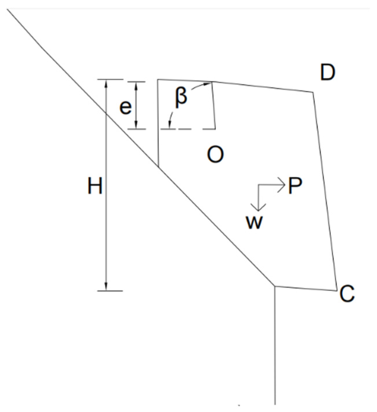
| Failure Mode of Dangerous Rock | Unstable | Basically Stable | Stable |
|---|---|---|---|
| Slump type dangerous rock | <1.0 | 1.0~1.3 | >1.3 |
| Tipping rock | <1.0 | 1.0~1.5 | >1.5 |
| Falling dangerous rock | <1.0 | 1.0~1.5 | >1.5 |
Disclaimer/Publisher’s Note: The statements, opinions and data contained in all publications are solely those of the individual author(s) and contributor(s) and not of MDPI and/or the editor(s). MDPI and/or the editor(s) disclaim responsibility for any injury to people or property resulting from any ideas, methods, instructions or products referred to in the content. |
© 2024 by the authors. Licensee MDPI, Basel, Switzerland. This article is an open access article distributed under the terms and conditions of the Creative Commons Attribution (CC BY) license (https://creativecommons.org/licenses/by/4.0/).
Share and Cite
Bai, M.; Cui, Z.; Mou, K. Early Detection and Stability Assessment of Hazardous Rock Masses in Steep Slopes. Appl. Sci. 2024, 14, 6317. https://doi.org/10.3390/app14146317
Bai M, Cui Z, Mou K. Early Detection and Stability Assessment of Hazardous Rock Masses in Steep Slopes. Applied Sciences. 2024; 14(14):6317. https://doi.org/10.3390/app14146317
Chicago/Turabian StyleBai, Mingzhou, Zhuangzhuang Cui, and Kai Mou. 2024. "Early Detection and Stability Assessment of Hazardous Rock Masses in Steep Slopes" Applied Sciences 14, no. 14: 6317. https://doi.org/10.3390/app14146317
APA StyleBai, M., Cui, Z., & Mou, K. (2024). Early Detection and Stability Assessment of Hazardous Rock Masses in Steep Slopes. Applied Sciences, 14(14), 6317. https://doi.org/10.3390/app14146317