Abstract
It is in the preliminary design phase of a project that the designer makes decisions concerning the global geometry of the structure. When working with space frames, the choice of the frame topology is key for the structural behavior. It is difficult to find manuals that provide guidance on which of the most common topologies is the right one for the project, let alone in wood construction. In response to this shortcoming, the use of parametric software is proposed (Grasshopper build1.0.0007 and Karamba 3D 2.2.0.16-220828). The aim is to create a dynamic catalog that responds instantaneously to changes in the parameters to provide information on structural behavior, pre-dimensioning and metrics. With the display of all this information, the architect will have enough technical argumentation to choose or reject options. The proposal is developed through a case study: the early design and analysis stages of flat double-layer timber spatial frames as for rectangular medium-span roofs.
1. Introduction
1.1. Space Frames
A space frame is often defined as a structural system designed from linear elements arranged in such a way that the transmission of forces is three-dimensional. This leads to an idea of opposition between spatial structures and so-called “flat” ones. However, the division between “flat” and “spatial” structures refers not to the structure itself, which is always spatial, but to the methods of analysis [1].
In planar systems, stresses are transmitted from the less rigid elements to the more rigid ones up to the foundations. On the way to the foundation, the forces become, as well as the section, larger and larger. On the contrary, in a space frame structure, all the elements contribute according to the three-dimensional geometry given to them, with no obvious force transfer sequence. In other words, the transmission of forces to the support is bifurcated in several elements so as not to have a concentration of forces in just a few elements.
The objective of this type of construction is to use the minimum amount of material to obtain lightweight structures without losing stiffness, stability and resistance. These are appealing structures not only from the engineering point of view, but also from the architectural one. These systems have led to the understanding of the building as a living being, as an organic structure, capable of adapting to the uncertainty of the future. There are approaches such as those of Louis Kahn, who plays with the natural growth of the spatial frames from the multiplication of the base spatial module. Another well-known project is the Fun Palace by Cedric Price and Joan Littlewood (Figure 1), a dismountable and reconfigurable artefact capable of housing any program that could respond to social needs. This logic is even extrapolated to the city and territory, giving rise to projects such as, among others, the megastructures of Archigram (Figure 1) or the three-dimensional urbanism of Yona Friedman.
Figure 1.
(a) Cedric Price, Fun Palace. (Source: toran, iv. https://www.flickr.com/photos/136374633@N04/23341131945/, accessed on 6 April 2023); (b) Archigram, Plug in City. (Source: Wyliepoon https://www.flickr.com/photos/wyliepoon/49224543288/, accessed on 7 April 2023).
In recent years, research has been carried out in several related areas. On the one hand, calculation methods have been proposed to measure the carbon emissions for the lifetime of the frames [2]. On the other hand, robotization processes are being developed for assembly and disassembly [3,4]. In this regard, a very promising line of research has been opened with respect to the possibilities of disassembly and reuse of the frames [5,6,7,8]. Given the current emerging context, this is a path that undoubtedly deserves to be investigated.
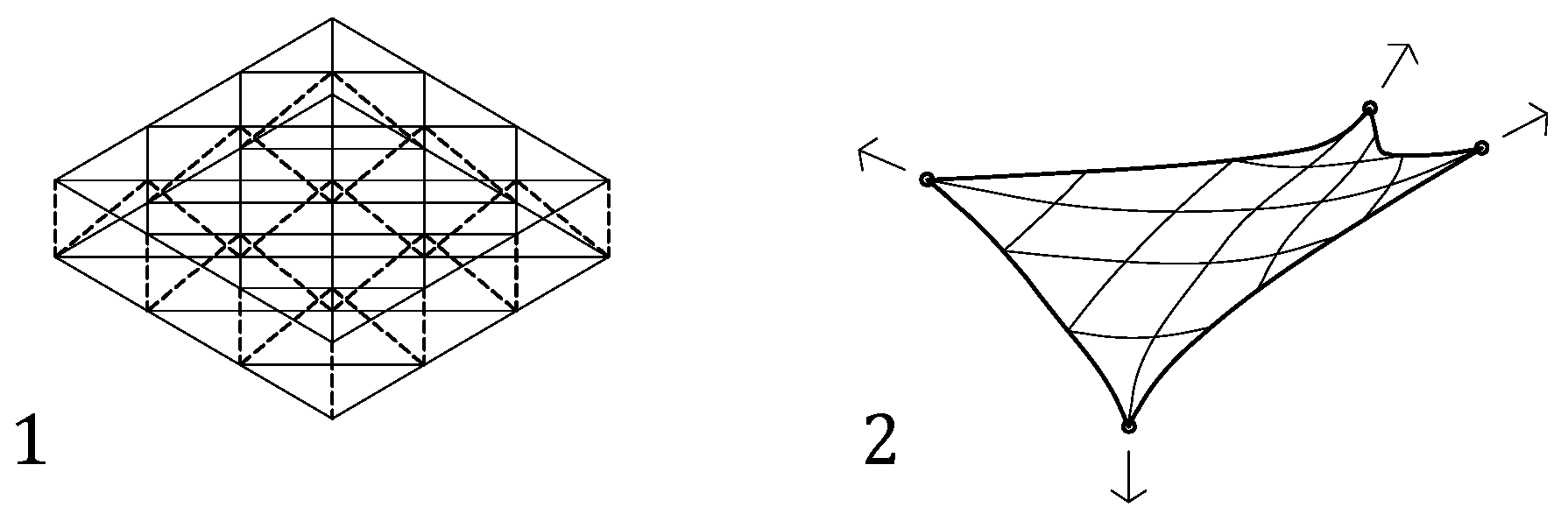
Back to the strictly structural-engineering aspect, spatial structures can be grouped into three main categories [9,10] (Figure 2):

Figure 2.
Space structure categories. (1) lattice discrete structure; (2) continuous structure.
- lattice discrete structures: they are based on discretization to create a more or less regular frame (grid, barrel vaults, domes, towers and free forms).
- continuous structures: a single surface acting as a membrane (slabs, shell, fabric).
- biform structures: combination of both discrete and continuous parts.
This paper will be centered on the first group for two main reasons:
- -
- Both planar and curved surfaces can be used. This research is focused on flat frames with the awareness that processes designed for a simple shape can be extrapolated to more complex ones. Parametrically, it is possible to apply any algorithmically designed process to any type of geometry.
That said, in shell structures, stiffness is achieved through shape. Their geometry directly derives from their flow of forces and defines their load-bearing behavior and lightness [11]. On the other hand, lattice spatial structures achieve resistance through cross-section. Being multiple-layer structures, the very composition of the sheet has a lever arm that stiffens them. By not being so form-dependent, the range of application of lattices is considerably wider, and that makes them appealing as the scope of this work.
- -
- A wide range of patented systems is available on the market. Even though most of them are aimed at metal construction, development in timber construction is also being accomplished. The main focus of the research is the node solution. It is at the joint where the stress transmission is concentrated and where the constructive requirements tend to reduce the cross-section of the timber bar. This contradiction poses a challenge in the development of the connection. It is, however, a difficulty that can be overcome, since timber construction is an option that looks very promising in the current climate crisis [3,6,7].
1.2. Construction Systems
Historically, space frames have belonged to the field of steel construction. Steel allows for thin sections without losing structural efficiency. Timber, while requiring care in the design of the joints, is also a suitable material for this type of system.
The present paper will focus on timber construction, and a brief state of the art is presented about the application of timber in space frames. The elements that form the spatial system will be developed individually as follows:
1.2.1. Bar Elements
This is an element in which the longitudinal dimension is of higher order than the other two. In the built examples, three types of wood bars have generally been used (Figure 3): bamboo bars (a), solid wood logs (b) and laminated timber sections (c1, c2).
Figure 3.
Bar element types. (a) bamboo bars; (b) solid wood longs; (c1) laminated timber section; (c2) laminated timber hollow section.
The first two groups belong to materials obtained directly from nature, and therefore, as in sawn timber construction, the shape and dimensions will not necessarily be optimized to the requirements of the project.
Regarding the third group, it is worth mentioning the contribution of the doctoral thesis of José Antonio Vázquez Rodríguez [12]. This work argues for the advantages of the shaping of bars by means of hollow sections of laminated timber (c2). The argument can be summarized in four points:
- -
- The hollow section equals the material’s value and offers less sensitivity to dimensional variations due to changes in environmental factors. Also, there is a reduction in risk against possible attacks of abiotic and biotic origin due to the fact that it is easier to carry out the integral treatment given its hollow character.
- -
- There is exploitation of the advantages offered by wood products in general and laminated ones in particular. It is a material that, due to its production process, has fewer imperfections and, therefore, a higher resistance performance. The same could be said of microlam (VLV).
- -
- The process of simple industrial execution consists of laminating rectangular pieces three or four times wider than the wall thickness of the hollow section so that, once the faces have been obtained by simple cutting, they can be glued against a master or guide piece and thus form the final piece. Consequently, the handling required is reduced, making the manufacturing cost competitive.
- -
- The square or rectangular hollow section is considered suitable for any type of frame, although it seems to be particularly suitable for the semi-octahedron frame.
1.2.2. Joints
Depending on the type of bar used, the joint solution also varies. In timber construction, the critical part seems to be the connection between the timber bar and the (usually metallic) node. It is where the joining elements weaken the timber section and, at the same time, where the highest stress concentration occurs. In this regard, some of the research that has been developed (or is still in progress) is shown below:
- -
- Bamboo connectors (Figure 4a): Ghavami and Moreira [13] developed a joint for the construction of double-layered bamboo space frames from octagonal plates welded to an octagonal base plate. During the research, the joint was tested on a double-layer bamboo space frame prototype with single supports every 4 m. The results were satisfactory. Currently, research is being continued with prototypes of larger spans.
 Figure 4. (a) Ghavami and Moreira’s bamboo frame connector; (b) Hybers’ solid wood log connector; (c) J.A. Vázquez’s glulam hollow section joint; (d) Finch, Marriage, Gjerde and Pelosi’s CNC fabrication frame with wood–wood joints.
 - -
- Solid wood log connectors (Figure 4b): One of the most well-known researchers in this field is Dr. Huybers [14]. Interested in the use of small-diameter logs, which, until then, had no use and were abundant in forestry waste, he developed a simple wire-tying method for attaching galvanized steel connector plates to the previously hollowed ends of roundwood poles.
Without going into much depth, some other joints that have been proposed are the KT-W joint by Katsuhiko Imai (University of Osaka) and the 14FTC-U joint by Alphose Zingoni (University of Cape Town).
- -
- Connectors in glulam sections (Figure 4c): In the same thesis [12] in which hollow sections of glulam are developed as bars, the appropriate joint solution for them is also uncovered. A hollow sphere is proposed with a screwed cover that allows access to the interior and incorporates unthreaded holes for inserting the threaded rods and fixing them inside the sphere by means of nuts. At the opposite end, the bar is threaded into an octagonal nut. To attach the node to the wood, casting plates are fixed to the inside of the wooden element.
- -
- Connectors by CNC fabrication (Figure 4d): So far, metal-to-wood joints have been presented. The node is usually made of a high strength steel, since the stress concentration is very high at that point. Steel is a material easily shaped to the desired geometry (spherical, cylindrical, etc.) and strong enough to resist this punctual concentration of forces.
A group of researchers from Victoria University of Wellington [15] proposed to work with plywood cut with the CNC router to create a wood–wood joint.
The results of the tests performed on the prototypes showed that this solution works with deformations of about 1/400 when overloads of use type A1 (residential zone housing) and B (administrative zones) are applied to it. Although the structure was not at its ultimate limit (collapse), it was concluded that the joint should be further stiffened.
Before moving on, we give one last note on the joints. Among the structures formed by bars, two subtypes can be distinguished: those in which the connection between bars is made through rigid nodes (that is, if the node undergoes a certain rotation, all the concurrent bars in it undergo the same rotation) or through articulated nodes (each concurrent bar can rotate independently of the others). This distinction, however, can often be overridden by the shape appearing when treating the nodes as rigid or as articulated, since the bending moments that necessarily appear in the first case are very small in comparison with the axial forces, which are of very similar magnitude in both cases. This consideration allows that it is not necessary to construct perfect articulated nodes and to use types of nodes that, in reality, are neither rigid nor articulated but are located, in general, in an intermediate zone [1,16].
1.2.3. Topology
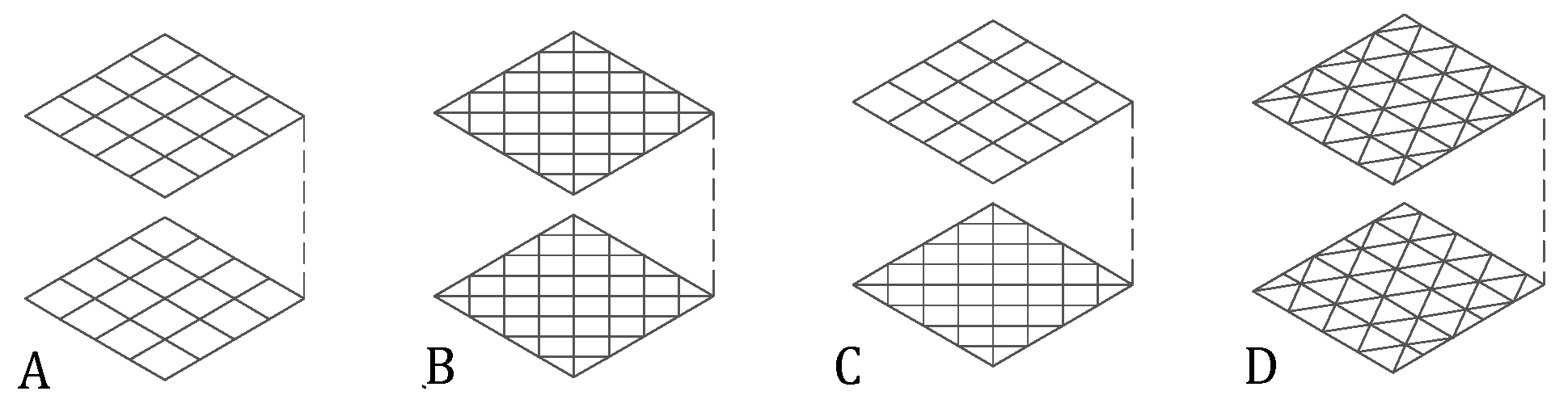
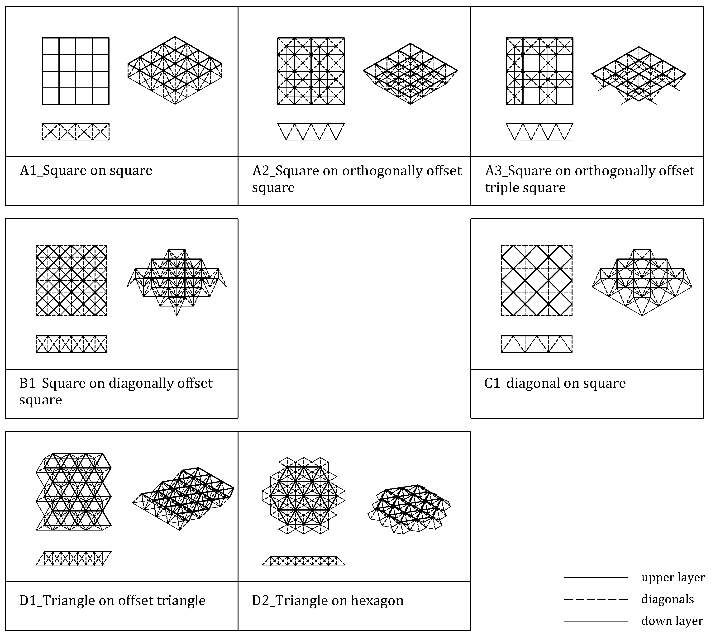
The topology refers to the geometrical order of the bars and nodes. For greater stiffness of the flat spatial frames (indispensable in large spans), two layers are arranged connected to each other through the set of diagonal bars. Although the variety of typology is practically infinite, the present work focuses on those patented and commercialized for use in construction. The use of a custom-designed topology would also involve the design of the construction system of joints and bars, an area that is not the focus of this work. Based on the bibliography [12,17,18,19,20,21], the seven most mentioned and used typologies have been chosen. A classification has been proposed (Figure 5). To order them, each one has been named with a letter and a number to be able to identify them easily throughout the paper (Figure 6).
Figure 5.
Frame topology classification. (A) group A; (B) group B; (C) group C; (D) group D.

Figure 6.
Analyzed topologies.
Group A: frames whose upper and lower layers are in parallel direction to the edges.
A1—Square on square: cubic module with vertical and diagonal bars. Absence of oblique diagonals.
A2—Square on orthogonally offset square: based on the pyramidal module with a square base. It is the most commonly used topology.
A3—Square on orthogonally offset triple square: based on the previous frame (A2), bars are suppressed in the lower layer in order to lighten it.
Group B: frames whose upper and lower layers are diagonal (45°) with respect to the edges.
B1—Square on diagonally offset square: pyramidal module frame with a square base arranged diagonally, at 45° to the edge.
Group C: frames in which one layer is parallel to the edges and the other diagonal (45°).
C1—Diagonal on square: created from the A1 frame, the top layer is given a 45° twist. It also has no oblique diagonals.
Group D: frames based on the triangular module.
D1—Triangle on offset triangle: created from the grouping of tetrahedral modules. It is the most rigid of the frames, as all the faces of the polyhedron are triangular, the undeformable geometry par excellence (Figure 7).
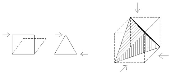
Figure 7.
Rigidity of the tetrahedral module.
D2—Triangle on hexagon: based on the D1 frame, the lower layer is lightened by removing bars to create equilateral hexagons.
The different topologies behave differently depending on the applied loads, the position of the supports and the size of the module. Further variations can be introduced by changing the size of the top chord grid relative to the bottom chord grid. Wider geometries are usually possible in the bottom layer of a double-layer frame because the members are normally in tension. That is, the lower tension chords may be longer than the upper compression members (no buckling effect).
1.3. Computational Design
Visual programming software allow the creation of parametric scripts without requiring any computer programming knowledge. This helps architects in the design process by lightening data management, automating repetitive tasks and producing simulations [22]. It is all about data management; the principles of the model are parameters that can be changed anytime. The most illustrative example is probably the upside-down model of churches by Antonio Gaudi. The designer created intricate catenary arches by suspended weighted strings. By adjusting the position of the weights (the parameter in this case), the shape of the catenary arches changed. This parametric model enabled Gaudi to analyze in real time the structural stability of his project. Nowadays, the process has been digitalized, but the concept remains the same [23].
In this regard, computational design is highly suitable for the design and analysis of both simple and complex modular timber structures, such as the ones discussed in this paper. Some authors [24] argue that, despite the evident advantages of these programs to produce freeform and aesthetically pleasing designs, the challenge in their application lies in the computational cost associated with the optimization of their layout and limitations in their fabrication. In that aspect, this paper wants to contribute by proving that geometrically simpler flat space frames are as worthy of parametric analysis as the more complex ones. There is value in using pre-established flat topologies because they have an industry backing them up and are not as dominant—speaking about architectural composition—as a form-finding method of geometry can be. Architects need assistance in early design stages to develop those simpler projects as well.
1.4. Objective
To sum up the ideas that have been presented in the introduction, the aim of this paper is to test the utility of parametric tools in the early design and analysis stages of flat wooden spatial frames.
To do so, a case study will be developed. All the topologies to be used are those mentioned in the literature on space frames [20,21,25]. They have patented construction systems and are available on the market. Even so, it is not easy to find the technical/commercial documentation necessary to design spatial frames in the preliminary design phase (much less in wood), and this work intends to fulfill this need.
This is why, in this case, the parametric tools are not used to obtain a geometry but to analyze which of the geometries offered by the market is the most suitable for the specific project. The idea is to create a file that gathers the mentioned topologies in a parametric way to generate and pre-dimension them at the request of the designer. The computer process offers the results in real time, and it is up to the designer to choose the best fit [26,27,28,29,30,31,32,33,34,35,36]. The case study will be a simulation of this process.
2. Materials and Methods
The chosen software for this work is Grasshopper (build 1.0.0007) [37], an extension of Rhinoceros 3D (version 7.24.22297.11002) [38] (NURBS-based 3D modeling software) for algorithmic modeling that allows the creation and parametric edition of geometries. Grasshopper also has another plugin called Karamba 3D (version 2.2.0.16-220828) [39], which enables finite element analysis and pre-dimensioning of the parametrized geometry.
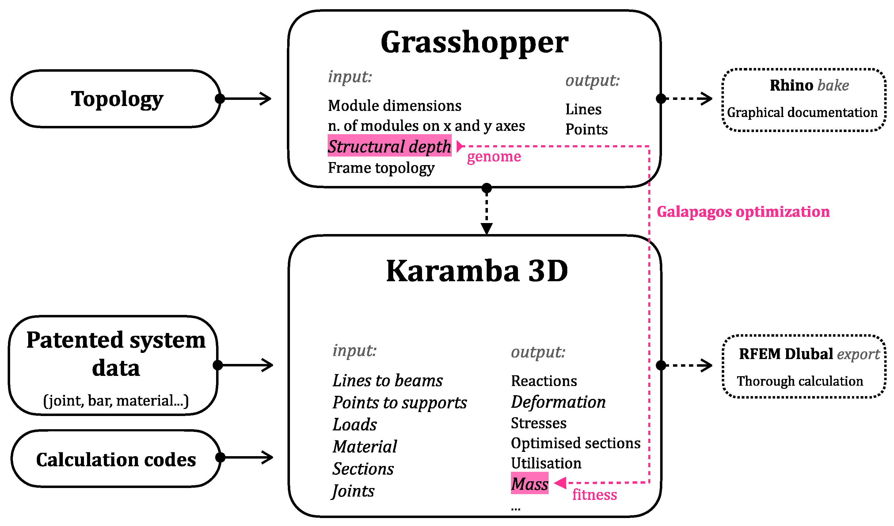
By combining the two software, it has been possible to create a “graphical calculation table” (Figure 8), which, by adjusting parameters such as dimensions and number of modules and choosing the topology (out of the 7 mentioned in Section 1.2.3 “Topology”), is able to compare results in real time and choose the combination that best suits the project. The geometry can also be imported into Rhino or AutoCAD to produce the graphical documentation.
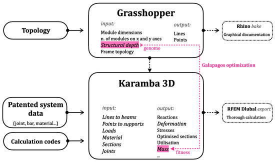
Figure 8.
Workflow diagram.
Although it is not within the scope of this work, it is worth mentioning that add-ons can be installed to Grasshopper in order to enable the bidirectional data exchange between the pre-dimensioned parametric model and the FEM software (three-dimensional finite element analysis software) for a deeper calculation. It is an added value to be able to perform all design and calculation phases with the same parametric model.
2.1. Creation of the Parametric Model
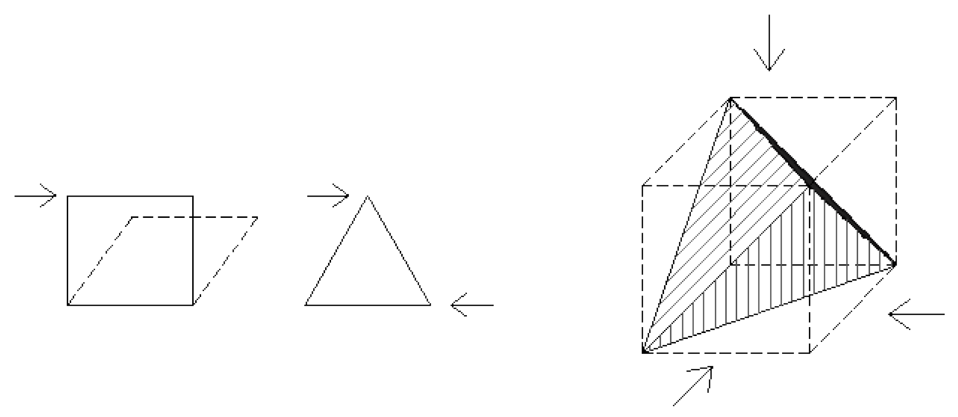
All the frames are parameterized based on the parameters summarized in Figure 9. In the case of triangular and hexagonal modules, being equilateral, the sides (L) of the modules are defined. Further details on the Grasshopper parametrization process will not be developed, as it is not the subject of this work.
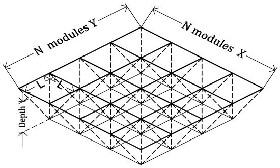
Figure 9.
Parameters in the file.
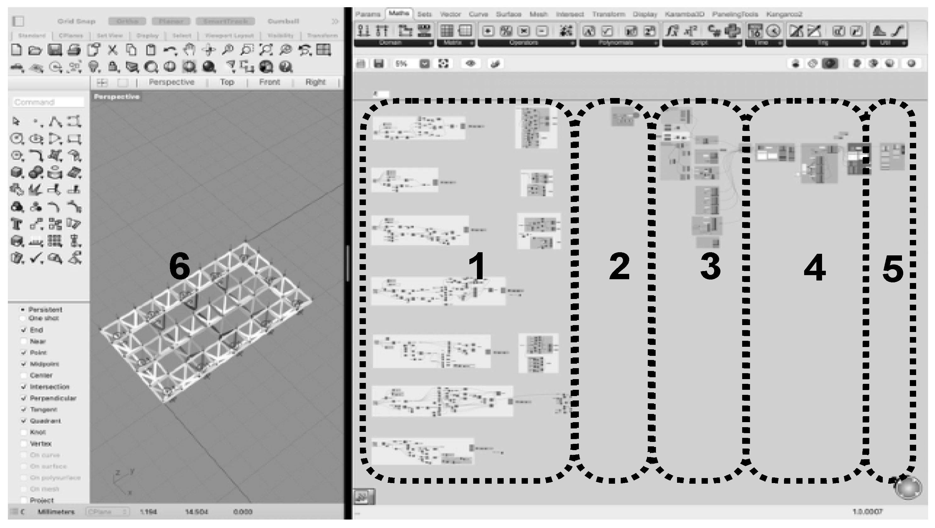
Figure 10 shows, on the right, a screenshot of the completed Grasshopper file and on the left, the Rhino viewer. The model is organized in the following groups (numbered in Figure 10):

Figure 10.
Screenshot of the Grasshopper file. (1) parametric definition; (2) parameters; (3) transformation from geometry to structure; (4) calculation; (5) visualization; (6) rhino viewer.
- parametric definition of the geometry of the frame: the 7 chosen frame topologies and their respective parameterized supports.
- grouping of the parameters: box grouping all the parameters to be chosen for the calculation, such as the frame topology, dimensions and number of modules and the depth.
- transformation from geometrical model to structural model: by entering data (loads, supports, material, cross-sections and joints), the chosen geometry (in the parameters grouping, 2) is translated into a finite element model.
- calculation and optimization: by means of Karamba 3D, the frame is calculated. Certain components (section optimization and genetic algorithms) are added to optimize the results.
- visualization of results: a command is given to visualize the results in the Rhino viewer (6).
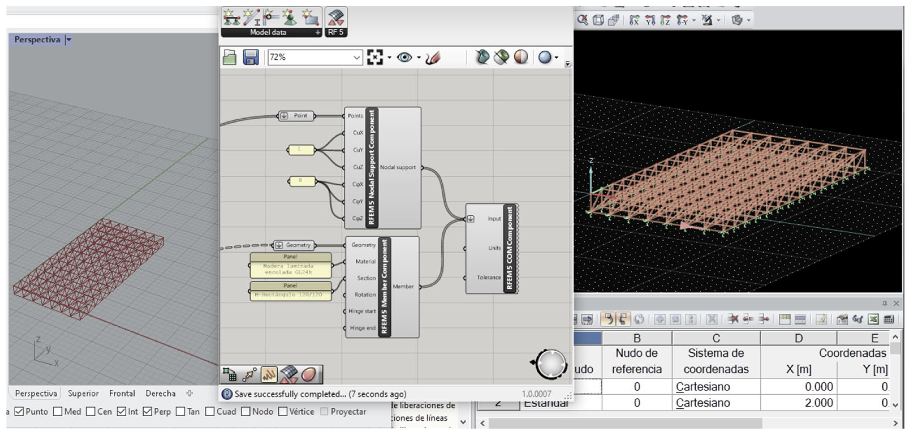
Before proceeding, a brief aside on the interoperability between FEM software and Grasshopper. A test has been performed using the interface of RFEM 6 Dlubal [40] (three-dimensional finite element analysis software) for Rhino and Grasshopper. Based on the existing Parametric FEM Toolbox plugin for RFEM 5, the RFEM 6 implements it by default. So by having the Grasshopper file and RFEM Dlubal opened side by side, and using the components that are shown in Figure 11, the connection is immediate. Changes in Grasshopper parameters are updated instantly in Dlubal as well. However, it must be emphasized that the transferred data are mainly geometrical (topology). The definition of sections and material must be performed using the exact terms of Dlubal for the program to process them correctly, and Karamba 3D components are not compatible. Therefore, this is a very useful feature in terms of handling the frame geometry (the main complexity of these structures) but somewhat limited for the rest (e.g., modeling hollow glulam bars). The remaining parameters for the complete calculation will be defined in the finite element program where the control of settings is considerably higher.
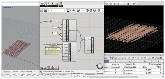
Figure 11.
Screenshot of Rhino 7 (left), Grashopper (center) and RFEM 6 (right) interconnected.
2.2. Optimization Components
The potential of Karamba has been explored through the use of its optimization components. Each of them will be explained as follows:
2.2.1. Cross-Section Optimization
Using the optimize cross-section component, the previously calculated model has been connected, and the lists of possible cross-sections have been added so that the program chooses the optimum cross-section for each member. The 90% depletion rate and the deflection limit L/300 (limitation defined in Section 4.3.3.1 of the CTE-DB-SE, standards based on Eurocode 5 [41]) have been defined. This module provides the data used in the results section and also when defining the “fitness” of galapagos (evolutionary solver inside Grasshopper).
2.2.2. Genetic Algorithm
The genetic algorithm (galapagos) works with 2 outputs: one or several genome(s) and a single fitness. The latter is the value to be minimized or maximized, and for this purpose, the program finds the appropriate value of the genome(s). A galapagos has been considered: genomes: structural depth—fitness: mass.
2.3. Data Entry
In order to enrich the comparison and identify the limits of each topology, two variables have been considered: roof dimensions and distribution of supports.
Four roof dimensions have been established, all related to the usual dimensions for the uses for which such roofs are usually intended:
- -
- 7 m × 12.5 m: In order to be able to analyze the behavior in relatively small spans, the 12.5 m dimension has been taken. This measure is the limit above which special transport is required. One of the advantages of space frames is that they are reduced to easily transportable bars and nodes regardless of the span they have to overcome.
- -
- 12.5 m × 25 m: medium spans, very common in light covers for semi-Olympic swimming pools, frontons, children’s playgrounds and so on.
- -
- 20 m × 40 m: As the work has developed, it has been considered necessary to add a roof of intermediate measures between 25 and 50 m, since many of the topologies do not reach 50 m but 40 m (with the following limitations: GL24h wood and maximum depth of 3 m).
- -
- 25 m × 50 m: large spans suitable for Olympic swimming pools, markets and so on.
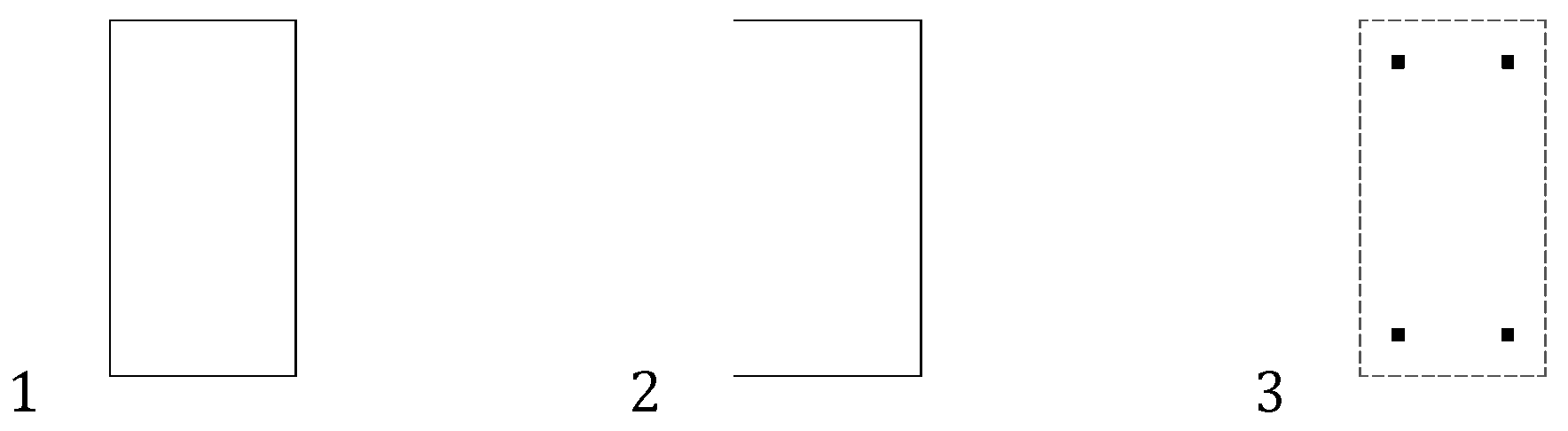
In order to study how the distribution of supports affects the structural behavior, 3 options have been considered (Figure 12):

Figure 12.
Support distribution options. (1) perimeter continuous support; (2) three-sided support; (3) four point support.
- perimeter continuous support: The most stable of all. The situation may occur that the facade of the covered space is the supporting element, and in such cases, this is the option to go for.
- three-sided support: All the roofs analyzed are rectangular in plan, and one of the longer sides has been freed to force the structure. This case is common in roofs for frontons, recreational areas, multi-purpose halls, etc., where the entire perimeter is closed except for one of the long sides.
- four point support: The two previous options correspond to continuous supports (walls/columns in a row); this, however, is the option to analyze the performance with 4 punctual supports uniformly distributed. In order to generate numerical results [42,43], a system of hollow glulam bars and a generic articulated joint has been simulated.
As a summary, Table 1 with all data entries is attached:

Table 1.
Data entry.

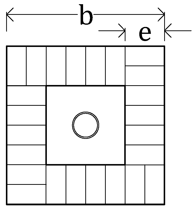
Figure 13.
Bar section model. (b) section total length; (e) section side wall thickness.
3. Results and Discussion
The results presented below intend to demonstrate the utility of the program in providing architects with information on structural behavior, pre-dimensioning and metrics. The data that can be extracted from the model are extremely abundant. Keeping in mind that the objective of the paper is to create a working tool rather than a particular solution of these structures, the results shown below are only an abstract, an example, of all the information that can be handled with this parametric file (which can certainly be extended).
The results will be organized in two phases:
- A first individual analysis, in which each frame is studied separately to obtain the optimal depth-to-span ratio by means of the genetic algorithm.
- A second comparative phase, where the results and data on the performance of each topology are collected for a comparative analysis. This will enable the identification of the range of use and limitation of each frame.
Before analyzing the results, a clarification about the data entry is required: the file created is intended to pre-dimension roofs of variable dimensions and geometry. With so much uncertainty, simplifications have been made on the safety side that affect the results:
- -
- Wind load: To avoid the extra parameterization of the pressure/suction areas defined by the CTE, the maximum load has been applied.
- -
- Application of the loads: To calculate the point load, instead of differentiating between edge, corner and center nodes, the same area (that of the center being the largest) has been applied equally to all nodes.
- -
- The joints are modeled as simple articulations, although the reality is that moments are always produced due to the lack of complete articulation. A developed calculation would involve nuancing the stiffness of the joint.
This parametric tool serves as a first draft of the structure, a quick way to discard options and arrive closer to the result. In the development of the specific project, other design programs should be used, for example, RFEM Dlubal (interfaced with the Karamba model), to further elaborate on the aspects that are not covered in this first step.
3.1. Individual Analysis
Optimal Depth for the Lowest Weight Possible
The galapagos algorithm has been used to determine the edge of each frame so that the mass is the minimum possible. Some authors [44] recommend an edge/modulus ratio between 0.5 and 1. They argue that lower ratios cause excessive stresses in the diagonal members, while higher ratios tend to increase the slenderness of these members forcing excessive buckling sizing. They conclude that, in general, in large-span structures with large stresses, it is desirable that the depth be close to the value of the modulus.
The results shown in Table 2 confirm the recommendation of the literature. All ratios are between 0.5 and 1, the average being 0.65. It can also be observed that as the module dimension increases, and therefore the span, the edge tends to increase and approaches the cubic ratio (edge = modulus value).
Table 2.
Galapagos mass–depth results.
For the comparative results that will follow, a middle term has been established: the ratio (0.866) which means that all the bars (upper, lower and diagonal layers) are of the same length. Besides avoiding buckling problems (that are not considered at this stage of the numerical calculation), comparisons can be made under the same circumstances for all the frames without being particularly restrictive for any of them, and it also facilitates assembly logistics.
3.2. Comparative Analysis
The objective of this section is to analyze the behavior and limitations of each frame and to define its range of use. Three topics will be studied:
- -
- Mass–deformation relationship: The relationship that summarizes the structural behavior of the frame. This shows how stiff the topology is and how much the section has to be increased to cover the required span (as it affects the mass).
- -
- Exhaustion rates: This indicates how close the bars are to their maximum stress capacity. In addition, it also detects when the structure is being optimally utilized and when the geometry does not allow the bars to work efficiently.
- -
- Metrics: Along with the structural behavior, the numbers of bars and nodes are collected for cost estimations.
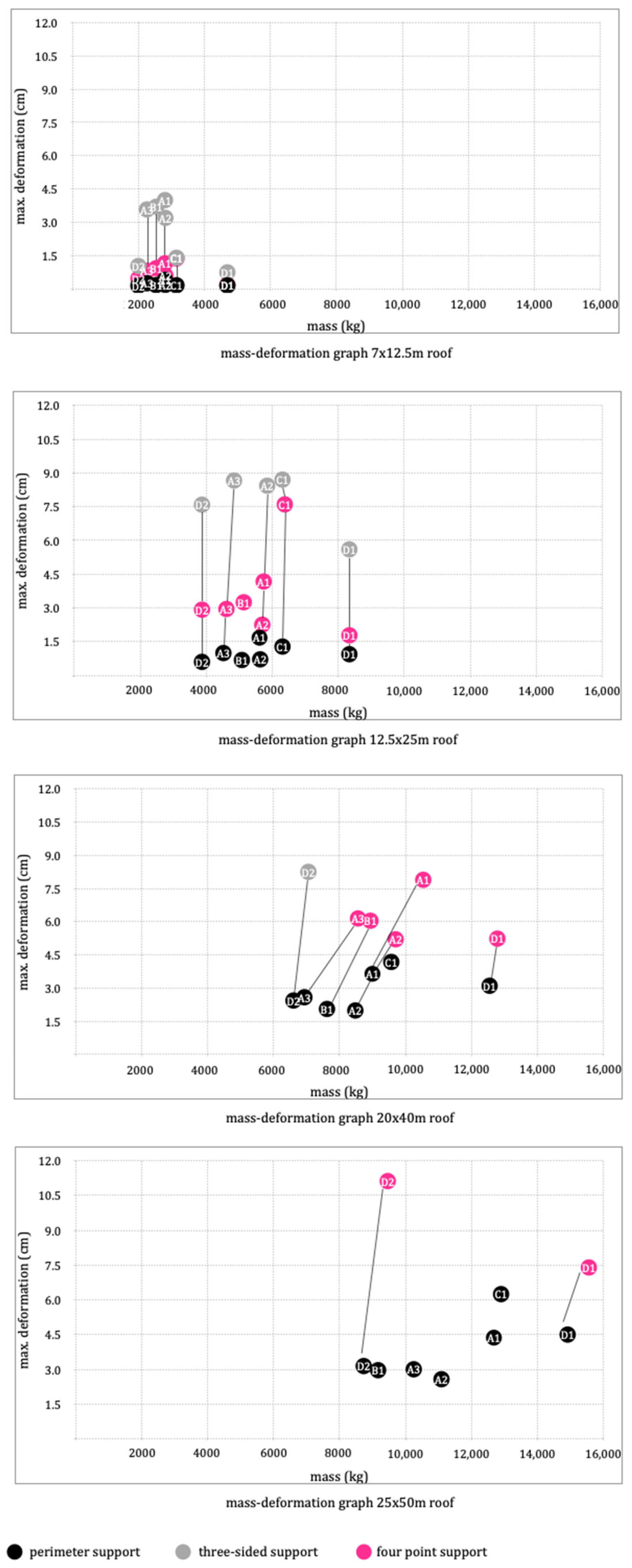
3.2.1. Mass–Deformation Ratio
The mass–deformation relationship has been studied under the following parameters: support distribution, topology of the frame and module dimensions.
In general, the three-sided support is the worst performing. From 20 to 25 m, the deformations are too large (only the D1 frame resists). The perimeter support, of course, has the best values, followed, not far behind, by the 4-point supports.
The change can be seen in the lines drawn on the graphs of Figure 14: in small spans (7 × 12.5 m), the mass remains constant (because it does not require section optimization), and it is the deformation that changes. Therefore, the line is vertical. As the spans increase, the line starts to recline (the 20 × 40 graph is the most illustrative of this process). The inclination becomes dramatically more severe at the jump from 12.5 × 25 m to 20 × 40 m. This slope demonstrates that the program has enlarged the frame sections to satisfy the L/300 deflection limit (hence the increase in mass), and thereby, the usefulness of the section optimization component is demonstrated.
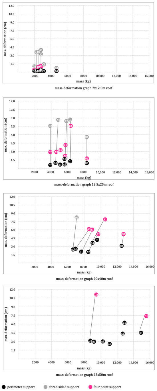
Figure 14.
Mass–deformation ratio result graphs.
Looking at the topologies individually, the D1 frame is the one with the highest mass in all cases and, at the same time, one of the least deformed. A1 and C1 are the worst performers, as they need a lot of mass without deformations decreasing too much. The others have similar behaviors, although the A2 and D2 frames behave slightly better.
3.2.2. Exhaustion Rates
The exhaustion rate is the ratio between the stress supported by the bar and the maximum strength of the material. A maximum exhaustion of 90% has been defined in Karamba. All optimizations have been made on this basis. The columns that do not appear are those that do not meet the calculation requirements. Something noteworthy in the graphs (Figure 15) is the development of the meshes D1 and D2. In 7 × 12.5 m roofs, they are well below the others. As the span is increased, they start to work up to the 90% limit.
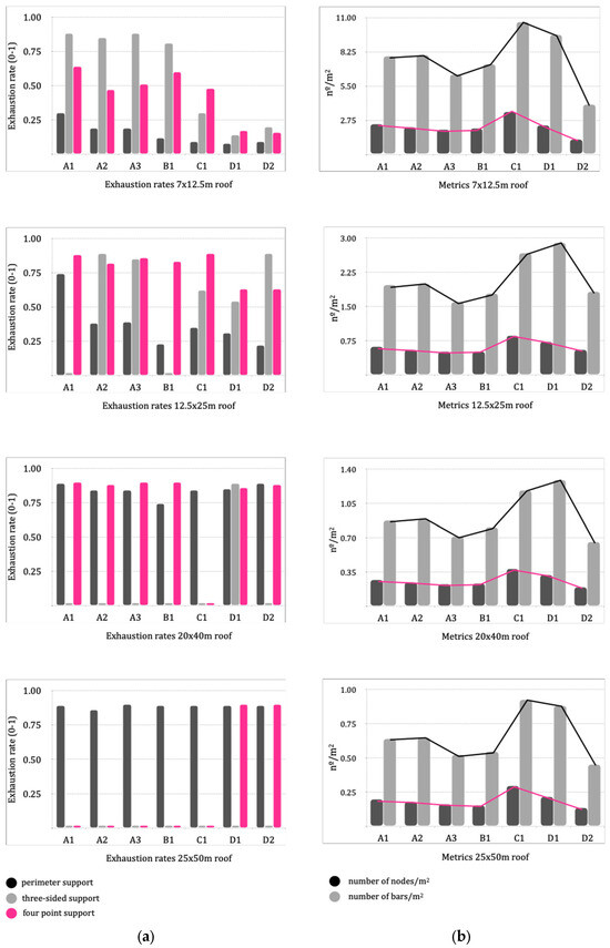
Figure 15.
(a) Utilization graphs; (b) metrics’ graphs.
3.2.3. Metrics: Nodes and Bars
As a guideline, a breakdown by components of the total cost of the system is estimated. These are the approximate average values [44]: bars 30%, nodes 40%, protection and paint 10% and assembly 20%. From these data, it can be deduced that the cost of a space frame is closely related to the type and number of joints (40% nodes+30% bars). Therefore, in the absence of a budget, the number of nodes can be taken as a guide to cost. In such a case, economizing means that the number of nodes per square meter should be kept to a minimum.
The graphs from Figure 15 show that frames C1 and D1 are the most “expensive” ones, both in terms of the number of nodes and number of bars, while A3 and D2, the lightened topologies, are the most cost-efficient ones. Frame A2 is in the middle of both extremes. As the span of the structure increases, the two lines marked on the graphs maintain their outline because the number of modules remains constant. However, numerically speaking, the structure becomes “cheaper”. The clearest example is to compare the values of the 7 × 12.5 and 25 × 50 roofs. Without going any further, the A1 mesh needs 2.46 nodes/m2 to cover 91 m2, while it only needs 0.2 nodes/m2 for 1200 m2.
By reducing the density of elements with longer bars, not only a greater load-bearing capacity is achieved, but also material and, therefore, cost is optimized. This is the advantage that space frames offer over other structural systems, and that is why they are so competitive in large spans.
4. Conclusions
4.1. Topologies
One of the objectives of the paper is to define the scope of each of the seven topologies, their strengths and limitations. After analyzing the results, the following conclusions are drawn:
- Group A (A1–A2–A3): These are the most balanced topologies, applicable in various situations. In this regard, it is only logical that they are the most common ones used. Of the three, A1 is the worst performer; its cubic module means that with the greatest number of nodes per square meter, it still has the greatest deformation.
- On the other hand, the semi-octahedral modulus provides A2 and A3 meshes with sufficient stiffness without affecting the mass too much. Between the last two, there is not that much difference; A3 turns out to be a good alternative to A2 when mass/economics is the determining factor, without serious detriment in deformations. In general, all three are relatively simple geometry topologies and easy to fit.
- Group D (D1–D2): their tetrahedral modulus makes them extremely rigid. Especially D1 is the preferred choice for large spans (over 40–50 m). From these spans on, the mesh starts to be competitive: the node-bar/m2 ratio decreases drastically (which makes them more cost-effective) and the depletion rates go up (which indicates that the structure is working). A future research task would be to further analyze the limits of tetrahedral meshes in larger spans (above 50 m).
- The D2 mesh is presented as a good alternative to D1. Although the lower layer detaches a significant number of bars to form hexagons, it is still a rigid mesh, competitive for its lightness (with deformations lower than those of mesh A3, also lightened). One drawback that can arise is the difficulty in handling the hexagonal geometry. If the project does not contemplate the use of these characteristic shapes from the beginning, edges and joints can become an added complication.
- B1: It can be a good alternative to A2 mesh. The metrics (number of bars and nodes) are better, and for what is saved in elements, the deformations do not increase so much.
- The only doubt that may come up is (as in the D2) the geometry itself. As the bars are not arranged parallel to the edges, bars of special lengths arise to finish off the mesh, problems that group A can avoid.
- C1: Of the seven topologies, C1 is the one that behaves the worst in general. It tends to destabilize easily, and it is comfortable up to a 20–25 m span. Beyond this limit, it becomes very limited. It is also the topology that needs more nodes and bars per square meter (slightly more than D1). In general, it seems that the geometry is not appropriate for generating a structural space frame.
It should be mentioned that in order to analyze the behavior of the topologies, the structure has been pushed to the limit. Some of the results collected in this paper, although complying with the standards, are quite tight (the deflections of the supports on three sides and the depletion indices). In the development of the calculation, the results should be handled more loosely, although for the purpose of this academic work, they are the appropriate ones.
Although the scope of the work has been flat meshes, the application of the system could be extrapolated from the plane to the curved surface and analyze, for instance, cylindrical or spherical meshes. This is a field to be explored in future projects.
4.2. Support Distributions
Another objective of the work is to analyze the repercussion of the different supports on the behavior of the structure. For this purpose, three cases have been considered: perimeter support, 3-sided support and four punctual supports. The following conclusions have been reached:
In general, the distribution of supports has a great influence on the structural behavior of the mesh, the change being less noticeable in the stiffer meshes (those of group D). Supports distributed in an orderly and symmetrical manner benefit the analyzed topologies. They do not tolerate mismatches and asymmetries well. Clearly, the perimeter continuous support is the most stable of all, although it is also limiting in the project. The four punctual supports offer the designer greater freedom.
The support on three sides is the most limiting. It is clear that the rectangular proportion (1/2) is not adequate in that case. Another future direction of the study would be to optimize the ratio of the roof to improve the values of the three-sided support. This would mean having to parameterize the lattices differently, so that changing the number of modules does not affect the overall dimensions of the roof. In this way, different ratios to 1/2 could be tested, using galapagos (fitness: arrow, genomes: number of modules on the x and y axis) to find the optimal ratio.
4.3. Using Grasshopper and Karamba
Understanding how information is handled between components is the most difficult part of Grasshopper, as it is a major shift from working with actual geometry to handling lists of data. Fundamental concepts such as “graft” and “flatten” become the cornerstone of modeling. The program is very powerful and useful. The genetic algorithm becomes an ally to obtain results without having to manually test the parameters, although the conditions must be well defined to avoid undesired results. It is also important to limit the number of variables so that the algorithm does not take too long to approach the answer (especially in these types of long files).
4.4. Final Conclusion
Although a workflow is proposed rather than specific numerical results, the case studies illustrate how much information this software can provide and thereby demonstrate their utility. In summary, a parametric analysis and pre-dimensioning tool has been created to project flat double-layer spatial meshes. A customizable and expandable “graphical spreadsheet” that accompanies the designer during the preliminary design phase.
Author Contributions
Conceptualization, M.M.-U., F.G.-Q. and J.A.B.-M.; Data curation, F.G.-Q. and J.M.R.-M.; Formal analysis, M.M.-U. and F.G.-Q.; Funding acquisition, F.G.-Q. and J.M.R.-M.; Investigation, M.M.-U.; Methodology, M.M.-U. and F.G.-Q.; Project administration, J.M.R.-M.; Resources, F.G.-Q., J.M.R.-M. and J.A.B.-M.; Software, M.M.-U. and F.G.-Q.; Supervision, F.G.-Q., J.M.R.-M. and J.A.B.-M.; Validation, F.G.-Q., J.M.R.-M. and J.B.A.; Visualization, M.M.-U., F.G.-Q., J.M.R.-M. and J.B.A.; Writing—original draft, M.M.-U.; Writing—review and editing, M.M.-U., F.G.-Q. and J.M.R.-M. All authors have read and agreed to the published version of the manuscript.
Funding
This research was funded by: 1. HAZI and the Basque Country Government, Vice-Ministry of Agriculture, Fisheries and Food Policy in the frame of the Timber Structures, Construction and Design Master. 2. University of the Basque Country. Architecture Department. 3. Fundación Tecnalia Research and Innovation.
Institutional Review Board Statement
Not applicable.
Informed Consent Statement
Not applicable.
Data Availability Statement
The data presented in this study are available in the article.
Conflicts of Interest
The authors declare no conflicts of interest.
References
- Margarit, J.; Buxadé, C.; Buxadé i Ribot, C.; Margarit, J. Las Mallas Espaciales en Arquitectura; Gustavo Gili: Barcelona, Spain, 1972. [Google Scholar]
- Xu, X.; You, J.; Wang, Y.; Luo, Y. Analysis and assessment of life-cycle carbon emissions of space frame structures. J. Clean. Prod. 2023, 385, 135521. [Google Scholar] [CrossRef]
- Robotic Manufacturing of Timber Space-Frames—DigitalFUTURES. Available online: https://digitalfutures.international/workshop/robotic-manufacturing-of-timber-space-frames/ (accessed on 12 March 2023).
- Huang, Y.; Garrett, C.R.; Ting, I.; Parascho, S.; Mueller, C.T. Robotic additive construction of bar structures: Unified sequence and motion planning. Constr. Robot. 2021, 5, 115–130. [Google Scholar] [CrossRef]
- Finch, G.; Marriage, G. Reducing Building Waste through Light Timber Frame Design. In Proceedings of the PLEA 2018 HONG KONG, Hong Kong, China, 10–12 December 2018. [Google Scholar]
- Koronaki, A.; Shepherd, P.; Evernden, M. Rationalization of freeform space-frame structures: Reducing variability in the joints. Int. J. Archit. Comput. 2020, 18, 84–99. [Google Scholar] [CrossRef]
- Finch, G.; Marriage, G.; Pelosi, A.; Gjerde, M. Applications and Opportunities for Timber Space Frames in the Circular Economy. In Proceedings of the CIB World Building Congress, Hong Kong, China, 17–21 June 2019. [Google Scholar]
- Bruun, E.P.G.; Adriaenssens, S.; Parascho, S. Structural rigidity theory applied to the scaffold-free (dis)assembly of space frames using cooperative robotics. Autom. Constr. 2022, 141, 104405. [Google Scholar] [CrossRef]
- Baverel, O. Nexorade: A Family of Interwoven Structures; University of Surrey (United Kingdom): Guildford, UK, 2000. [Google Scholar]
- Gutiérrez-Astudillo, N.C.; Flores, A.; Preciado, A. Reciprocal frame structures, a first academic approach to sustainable structures. In Proceedings of the IASS Annual Symposia, Tokyo, Japan, 26–30 September 2016; Available online: https://www.semanticscholar.org/paper/Reciprocal-frame-structures%2C-a-first-academic-to-Guti%C3%A9rrez-Astudillo-Flores/bad4f5510e8ebd89e009c3bd8d9762e3132616e5 (accessed on 25 April 2023).
- Adriaenssens, S.; Block, P.; Veenendaal, D.; Williams, C. (Eds.) Shell Structures for Architecture: Form Finding and Optimization; Routledge: London, UK, 2014; ISBN 978-1-315-84927-0. [Google Scholar]
- Vázquez, J.A. Las Barras Huecas de Madera en la Construcción de Estructuras Espaciales; Universidade da Coruña: La Coruna, Spain, 2001. [Google Scholar]
- Ghavami, K.; Moreira, L.E. 61. Double-layer bamboo space structures. In Space Structures 4; Thomas Telford Publishing: London, UK, 1993; ISBN 978-0-7277-4941-3. [Google Scholar]
- Huybers, P. Palos de madera como elementos de estructuras espaciales. Rev. Digit. Cedex 1990, 79, 99. [Google Scholar]
- Finch, G.; Marriage, G.; Gjerde, M.; Pelosi, A. Experiments in Timber Space Frame Design: Fabrication, Construction and Structural Performance. In Proceedings of the 24th International Conference of the Association for Computer-Aided Architectural Design Research in Asia (CAADRIA), Hong Kong, China, 15–18 April 2019. [Google Scholar]
- Lan, T.T. Space Frame Structures; CRC Press: Boca Raton, FL, USA, 1999. [Google Scholar]
- Mupona, G.T. Development of Space Truss Systems in Timber. Master’s Thesis, Faculty of Engineering and the Built Environment, University of Cape Town, Cape Town, South Africa, 2004. Available online: https://www.semanticscholar.org/paper/Development-of-space-truss-systems-in-timber-Mupona/211102da0a241e41447b23fcb658ca3a7b9fd99b (accessed on 12 March 2023).
- Moggio, N. Glued Laminated Timber Space Truss Systems. Master’s Thesis, Università di Trento, Trento, Italky, 2012. Available online: http://lup.lub.lu.se/student-papers/record/3131142 (accessed on 12 March 2023).
- Álvarez Pablos, J. Mallas Planas y Cilíndricas de Módulos Apilables de Madera Laminada; Universidade da Coruña. Escola Técnica Superior de Arquitectura: La Coruna, Spain, 1998; ISBN 978-84-692-8073-7. Available online: https://ruc.udc.es/dspace/handle/2183/5561 (accessed on 12 March 2023).
- Chilton, J. Space Grid Structures; Architectural Press: Oxford, UK, 2000; ISBN 978-0-7506-3275-1. [Google Scholar]
- Eekhout, M. Architecture in Space Structures; Uitgeverij 010 Publishers: Rotterdam, The Netherlands, 1989; ISBN 978-90-6450-080-0. [Google Scholar]
- Aksöz, Z.; Preisinger, C. An Interactive Structural Optimization of Space Frame Structures Using Machine Learning. In Impact: Design with All Senses; Gengnagel, C., Baverel, O., Burry, J., Ramsgaard Thomsen, M., Weinzierl, S., Eds.; Springer International Publishing: Cham, Switzerland, 2020; pp. 18–31. [Google Scholar]
- Jormakka, K. Basics Design Methods; Birkhäuser: Basel, Switzerland, 2017; ISBN 978-3-0356-1147-2. [Google Scholar]
- Koronaki, A.; Shepherd, P.; Evernden, M. Layout Optimization of Space Frame Structures. In Proceedings of the IASS Annual Symposium 2017, Hamburg, Germany, 25–28 September 2017. [Google Scholar]
- Gordon, J.E. Estructuras o Por qué las Cosas no se Caen, 2nd ed.; Calamar: Madrid, Spain, 2004; ISBN 978-84-96235-06-9. [Google Scholar]
- De Moraes, M.H.; Fraga, I.; Junior, W.; Christoforo, A. Comparative analysis of the mechanical performance of timber trusses structural typologies applying computational intelligence. Rev. Árvore 2022, 46, e4604. [Google Scholar] [CrossRef]
- Apolinarska, A.A. Complex Timber Structures from Simple Elements: Computational Design of Novel Bar Structures for Robotic Fabrication and Assembly. Ph.D. Thesis, ETH Zurich, Zürich, Switzerland, 2018. [Google Scholar]
- Andrén Jakobsson, N.; Bohman, S. A Generative Design of Timber Structures according to Eurocode. Development of a Parametric Model in Grasshopper; KTH Royal Institute of Technology: Stockholm, Sweden, 2019; Available online: http://urn.kb.se/resolve?urn=urn:nbn:se:kth:diva-255661 (accessed on 12 March 2023).
- Almaraz, A. Evolutionary Optimization of Parametric Structures: Understanding Structure and Architecture as a Whole from Early Design Stages. Master’s Thesis, University of A Coruña, La Coruna, Spain, 2015. Available online: https://ruc.udc.es/dspace/handle/2183/15965 (accessed on 12 March 2023).
- Martínez Villarroya, D. Arquitectura Fractal: Optimización Topológica. Available online: https://oa.upm.es/55874/ (accessed on 12 March 2023).
- Muñoz Ávila, D.A. Implementación de un Algoritmo de Optimización Multi—Objeto de una red de Barras Utilizando un Lenguaje de Programa-ción Visual en “Rhinoceros’ y sus Extensiones. 2021. Available online: https://repositorio.uisek.edu.ec/handle/123456789/4519 (accessed on 12 March 2023).
- Navarro Mateu, D. Procesos Naturales Aplicados a la Arquitectura Mediante Computación: Ciencia Evo-Devo y Modelado Algorítmico a Través de Grasshopper. Ph.D. Thesis, Universitat Internacional de Catalunya, Barcelona, Spain, 2017. Available online: https://www.tdx.cat/handle/10803/552427 (accessed on 12 March 2023).
- Villar Monteagudo, I. Estudio Paramétrico Sobre Mallas de Doble Capa. 2015. Available online: https://ruc.udc.es/dspace/handle/2183/16171 (accessed on 12 March 2023).
- Weldegiorgis, F.; Dhungana, A.R. Parametric Design and Optimization of Steel and Timber Truss Structures: Development of a Workflow for Design and Optimization Processes in Grasshopper 3D Environment. 2020. Available online: http://urn.kb.se/resolve?urn=urn:nbn:se:kth:diva-277901 (accessed on 12 March 2023).
- Yan, X.; Bao, D.; Zhou, Y.; Xie, Y.; Cui, T. Detail control strategies for topology optimization in architectural design and development. Front. Archit. Res. 2022, 11, 340–356. [Google Scholar] [CrossRef]
- Preisinger, C. Linking Structure and Parametric Geometry. Archit. Des. 2013, 83, 110–113. [Google Scholar] [CrossRef]
- Network, Scott Davidson Created This Ning Network. Grasshopper. Available online: https://www.grasshopper3d.com/ (accessed on 29 April 2023).
- Associates, Robert McNeel & Associates. Rhinoceros 3D. Available online: https://www.rhino3d.com/es/ (accessed on 29 April 2023).
- Karamba3D. Available online: https://karamba3d.com/ (accessed on 29 April 2023).
- Software Para Análisis Estructural y Dimensionado|Dlubal Software. Available online: https://www.dlubal.com/es (accessed on 29 April 2023).
- UNE-EN 1995-1-1:2016 Eurocódigo 5. Proyecto de Estructuras de Madera. Parte 1-1: Reglas Generales y Reglas para Edificación. Available online: https://www.une.org/encuentra-tu-norma/busca-tu-norma/norma?c=N0056510 (accessed on 1 May 2023).
- Muñoz-Vidal, M. Generación y Cálculo de Mallas Espaciales; Universidad, Departamento de Tecnolog’ia de la Construcción: La Coruña, Spain, 1993. [Google Scholar]
- Navarro Carrasco, S. Cálculo Estructural de Una Gran Marquesina Espacial Ejecutada Íntegramente Mediante una Malla Espacial de Doble Capa de Acuerdo con los Eurocódigos que Disponen de Anejo Nacional; Cartagena, Spain. 2015. Available online: https://repositorio.upct.es/handle/10317/4912 (accessed on 12 March 2023).
- Cavia-Sorret, P. Las mallas espaciales y su aplicación en cubiertas de grandes luces. Re. Rev. De Edif. 1993, 15, 7–15. [Google Scholar] [CrossRef]


Disclaimer/Publisher’s Note: The statements, opinions and data contained in all publications are solely those of the individual author(s) and contributor(s) and not of MDPI and/or the editor(s). MDPI and/or the editor(s) disclaim responsibility for any injury to people or property resulting from any ideas, methods, instructions or products referred to in the content. |
© 2024 by the authors. Licensee MDPI, Basel, Switzerland. This article is an open access article distributed under the terms and conditions of the Creative Commons Attribution (CC BY) license (https://creativecommons.org/licenses/by/4.0/).