Aerodynamic Analysis of Fixed-Wing Unmanned Aerial Vehicles Moving in Swarm

Abstract

This paper presents a close-formation flight of two unmanned aerial vehicles (UAVs) and the aim of the study is to improve the understanding of the vortex effects between fixed-wing UAVs in a swarm using computational fluid dynamics (CFD) tools. To validate the numerical method, results of a variable-density wind tunnel test from the literature were used. This numerical CFD analysis was used to determine the lift coefficient (C_L) and the drag coefficient (C_D) values for a single UAV at various angles of attack. When examining the aerodynamic impact areas behind the UAV, the longitudinal distance between the two UAVs is not particularly effective for close flight. Therefore, CFD analyses were carried out on the two UAVs for both vertical and lateral distances. The optimum position for close-formation flight was identified using C_L/C_D ratios. The results of the analysis indicate that the most effective flights, across all lateral positions, occur when the two UAVs are vertically at the same height. In terms of aerodynamic efficiency, the most effective points for close-formation flight for wingspan b are at lateral distances of 0.875 b and 1 b. At these positions, flight efficiency can be increased by approximately 11.5%.

1. Introduction

Unmanned aerial vehicles (UAVs) have been widely used in military and civilian applications during the last few decades, including mapping, aerial cinematography, search and rescue operations, surveillance, and reconnaissance. Because of their increased sensing range, computing power, and weaponry, UAV swarms operating in formation perform better than a single UAV in challenging and dynamic mission settings [1].

The formation flying of birds serves as an inspiration for researchers studying aircraft flight. It is commonly known that during migration, birds can extend their range and endurance by flying in a V-formation. Using a basic aerodynamic model, Wieselsberger [2] conducted the first investigation into formation flight through an aerodynamic theoretical approach in 1914. He came to the conclusion that the V-formation would be ideal for approaching equipartition of drag. Lissaman and Schollenberger [3] discovered that a group of 25 birds could expand their range by 71% when compared to a single bird.

In an effort to enhance aerodynamic performance in aviation, researchers have spent a great deal of time studying how migratory bird species, which fly in closely spaced groups, might fly in formation. Research incorporating flight testing has demonstrated the fuel-saving benefits of close flying in V-formation. Two F/A-18 aircraft were used in formation flight experiments by Hansen and Cobleigh [4]. The findings indicate that at the ideal position, the drag of trailing aircraft reduces by almost 22%. In a two-aircraft formation flight experiment, Pahle et al. [5] investigated the effects of the lead’s vortex on C-17 large transport-class vehicles. The results of the flight data indicate that formation flight reduces engine thrust and fuel flow by more than 10% and saves more energy than the single flight. In actuality, these formation-flight studies are expensive and risky.

The Vortex Lattice Method (VLM) is a numerical method to examine aerodynamic effects without risky and expensive experiments. In the literature, there are studies on close-formation flight with novel proposals based on the VLM [6,7,8]. Blake and Gingras [9] discovered that the highest induced drag reduction was 25–40% with a VLM approach, which was validated by wind tunnel test results. Trumic and Swamy [10] showed that the VLM results are overpredicted in lift coefficients and underpredicted in drag coefficients compared to CFD results, especially at high angles of attack. Although the aerodynamic analyses in this study were performed for single flight and not for swarm flight, this study is important in the context of comparison. While the VLM is a relatively simple method, analysis with CFD tools is more powerful because it includes the viscosity effect.

There are many studies in the literature to determine the aerodynamic implications of swarm formation flight. Cui et al. [11] designed a two-aircraft flight formation consisting of blended wing body (BWB) aircraft flying in a V-formation. CFD was used to perform a numerical simulation of the aerodynamic interaction during two-aircraft-formation flying. When considering the balance of lift and gravity, the trailing aircraft has a notably high drag reduction of 25.1%. An optimization technique for a close-formation flight with two BWB aircraft was presented by Yang et al. [12]. In order to confirm the accuracy of the CFD method’s results, including the mesh transformation technique, a low-speed wind tunnel test was performed. According to the optimized results, the lift-to-drag ratio of the trailing aircraft reaches its highest value 24.7%. The optimum position for this value is achieved by flying the trailing aircraft vertically 2.2% of the wingspan below and horizontally 14.7% of the wingspan away from the leader aircraft. According to the study, in close-formation flight, the trailing aircraft’s aerodynamic performance is insensitive to longitudinal span but sensitive to lateral and vertical span. Zhang et al. [13] used CFD to simulate the aerodynamic properties of close-formation flight for swarms of BWB-model UAVs. The study’s findings demonstrated that, with a maximum increase of 25.4% over a single flight, the ideal position for the UAV to produce the maximum lift-to-drag ratio is at z/b = 0 and y/b = 0.75 (where z is the vertical distance, y is the lateral distance, and b is the wingspan). The study also proposed that the flow field behind the UAV will be more complex if it has the combination of a vertical and a horizontal tail. Shin et al. [14] used the CFD approach to evaluate the aerodynamic properties of a BWB aircraft swarm flight. On the other hand, different analyses were performed on flights that had more than four, five, or seven elements. The study also examined the echelon formation in addition to the V-formation. Specifically, studies utilizing CFD analysis have typically used simpler geometries, such BWB, in their execution. In these investigations, the aircraft speeds are 0.7 Ma and higher.

This study examines the aerodynamic effect between swarming UAVs using CFD analysis. In contrast to previous research in the literature, a UAV model including a fixed-wing with tail is used for geometry. It is preferred to adopt a tactical UAV model known as the Medium-Altitude Long-Endurance (MALE) class, which is currently employed in numerous military and civilian industries. When compared to studies in the literature, the speed value used in the analysis Is low because it was determined based on the UAV’s model real-flight properties. The goal is to ascertain the close-formation flight performance values in V-formation for these commonly used UAVs. Data validation with analysis on a three-dimensional wing, a single UAV model’s analysis and impact area determination, and analysis of two UAVs in different positions make up this study.

2. Materials and Methods

The ANSYS Fluent program was employed for CFD analysis through the ANSYS Workbench interface. The modular design of the Workbench makes it possible to run multiple software packages together. All software packages used were taken from the content of ANSYS 2023 R2 edition. The computer on which CFD analyses were performed has an i9 processor, 24 cores, and 64 GB RAM.

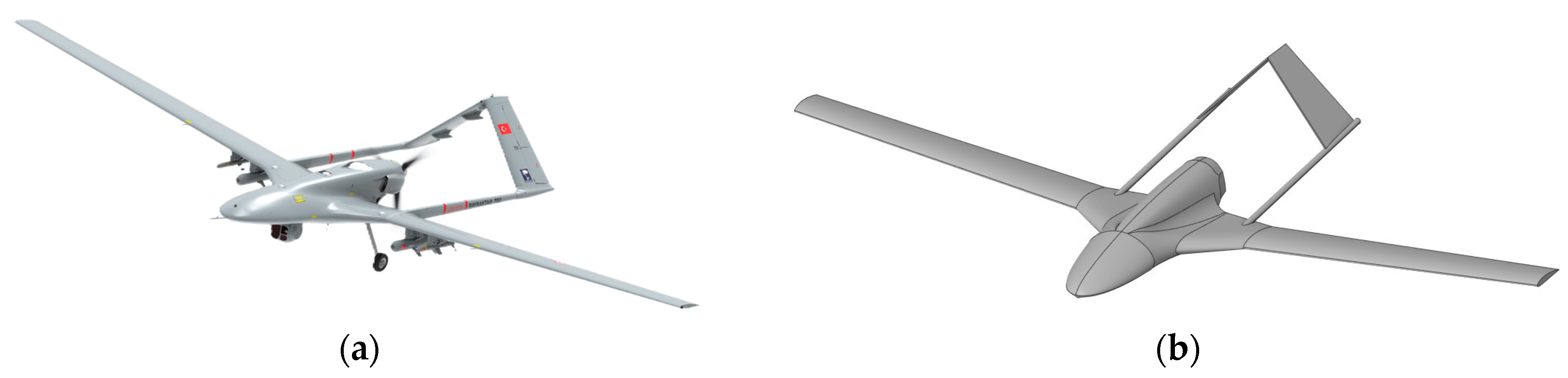
2.1. Geometry

In this study, we opted for a MALE UAV. This model has a boom-mounted inverted V-tail and is without winglets on the wings. MALE UAVs, which are smaller, more manageable, and less expensive to produce, deploy, and operate than larger UAVs, have the capacity to transport multiple kilograms of payload equipment. This equipment can range from humanitarian aid to advanced electronics. Currently, MALE UAVs dominate the market in terms of market share, as indicated by recent research [15]. The model’s geometry was derived using a real vehicle’s primary dimensions and its available images. The geometry was generated using the SpaceClaim software. The geometry is simplified, and the propeller motor is not included. Figure 1 shows the image of the real model, as well as the generated simplified geometry. However, the airfoil information is not accessible owing to proprietary knowledge restrictions for the real model. The airfoil chosen is the NACA 4415 developed by National Advisory Committee for Aeronautics which is a United States agency. According to Shunshun and Zheng’s [16] research, the NACA 4415 is recommended for use in MALE UAVs because of its favorable attributes of low speed and low drag. Furthermore, just a few studies in the currently available field of research have used this specific airfoil design in the setting of MALE UAV configurations [17,18].

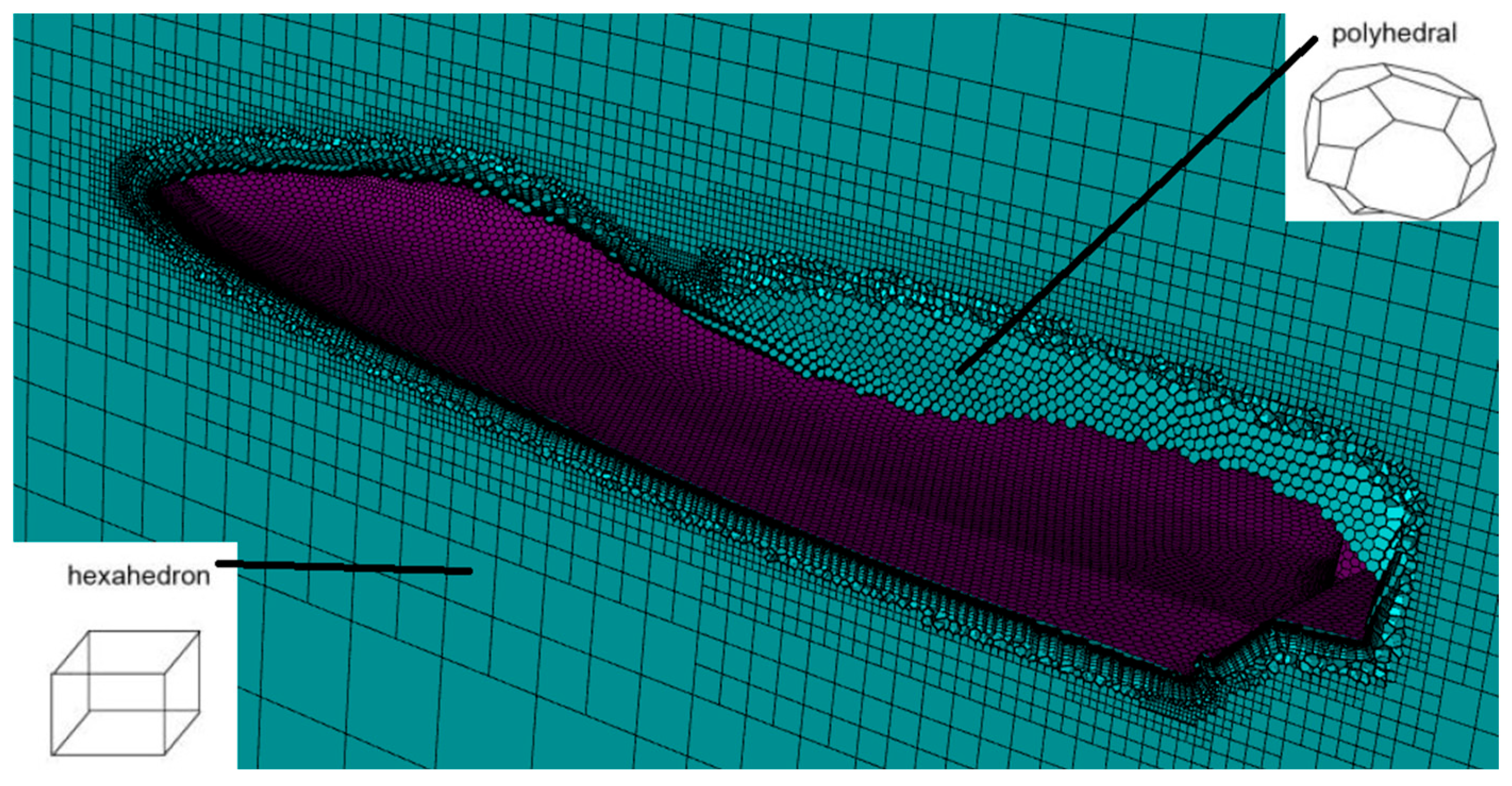
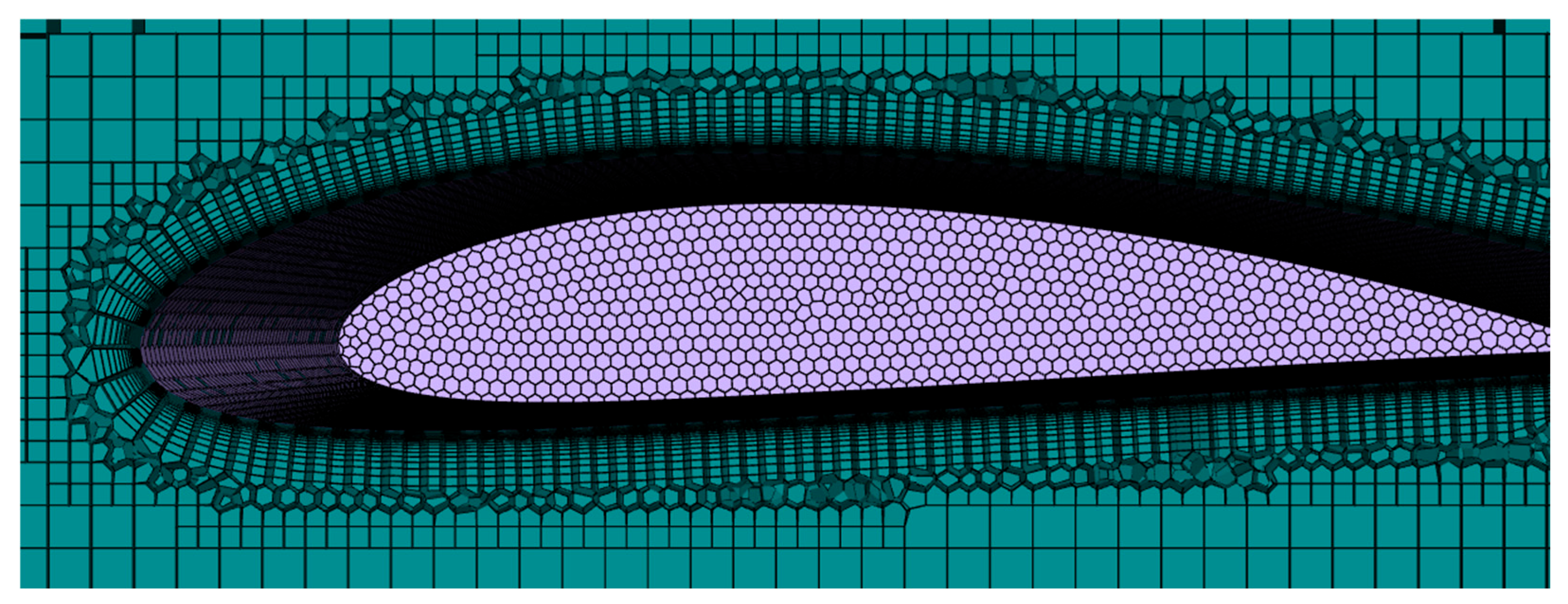
2.2. Meshing

The Fluent Meshing software was utilized for the process of meshing, and the specific reason for this preference is its capability to generate meshes using the poly-hexcore option. The poly-hexcore method is a hybrid approach that combines a combination of polyhedral and hexahedral element types and effectively addresses specific requirements by employing those types of elements. The polyhedral and hexahedral element types are illustrated in Figure 2. The poly-hexcore approach proves particularly advantageous in aerodynamic and hydrodynamic investigations, offering benefits such as reduced element count, faster convergence, and improved accuracy [19]. It is a useful technique for meshing complex geometries with boundary layer approximation, just as in the present study.

2.3. Governing Equations

The solver used is Fluent, which is CFD software that utilizes a finite volume method to solve the complete Reynolds-averaged Navier–Stokes (RANS) equations [20]. The finite volume solver is used for numerical simulations to solve the three-dimensional Navier–Stokes (N-S) equations. N-S equations embody the fundamental concepts of mass and momentum preservation for a fluid in motion. The utilization of a turbulence model entails the substitution of the N-S equation with the RANS equation. The continuity equation and RANS equations for steady, incompressible, and turbulent flow can be expressed as follows [21]:

$${\displaystyle \frac{\partial \rho }{\partial t}}+{\displaystyle \frac{\partial }{\partial x_i}}\left(\rho u_i\right)=0,$$

(1)

$${\displaystyle \frac{\partial }{\partial t}}\left(\rho u_i\right)+{\displaystyle \frac{\partial }{\partial x_i}}\left(\rho u_i{u}_j\right)=-{\displaystyle \frac{\partial \rho }{\partial x_i}}+{\displaystyle \frac{\partial }{\partial x_j}}\left[\mu \left({\displaystyle \frac{\partial u_i}{\partial x_j}}+{\displaystyle \frac{\partial u_j}{\partial x_i}}-{\displaystyle \frac{2}{3}}{\delta }_{ij}{\displaystyle \frac{\partial u_i}{\partial x_j}}\right)\right]+{\displaystyle \frac{\partial }{\partial x_j}}\left(-\overline{\rho {u\prime }_i{u\prime }_j}\right),$$

(2)

Here, ρ is the density of air, t is the time, µ is dynamic viscosity, and u_i is the velocity components. The last term in the equation (−ρu_i′u_j′) indicates Reynolds turbulence stress. There is no analytical way to determine these values because turbulence is chaotic. The turbulence stresses in the momentum equation are computed using turbulence models. To compute these values, turbulence models have been constructed [21].

The most commonly used turbulence models in CFD analysis are the Spalart–Allmaras, k-ε, and k-ω turbulence models. The Spalart–Allmaras model is a one-equation turbulence model. Both k turbulence models are two-equation models. Although a one-equation solver is a low-cost model, two-equation models can meet the accuracy requirements of most flow problems. Also, the k-ω turbulence model has two types, Standard and Shear Stress Transport (SST). The k-ω SST turbulence model is applied in this work. The k-ω SST two-equation model can simulate large separation flow by combining the k-ε and k-ω two-equation models through a mixing function. This allows the model to fully utilize the advantages of the k-ε model for free flow and the k-ω model restricted flow on the wall [11]. Developed by Menter [22], the SST model makes use of the following equations for turbulent kinetic energy (k) and specific dissipation (ω):

$${\displaystyle \frac{\partial k}{\partial t}}+{\displaystyle \frac{\partial }{\partial x_j}}\left(k{U}_j\right)={\tau }_{ij}{\displaystyle \frac{\partial U_i}{\partial x_j}}-{\beta }_k\omega k+{\displaystyle \frac{\partial }{\partial x_j}}\left[\left(v+{\displaystyle \frac{v_t}{{\sigma }_k}}\right){\displaystyle \frac{\partial k}{\partial x_j}}\right],$$

(3)

$${\displaystyle \frac{\partial \omega }{\partial t}}+{\displaystyle \frac{\partial }{\partial x_j}}\left(\omega U_j\right)={\displaystyle \frac{\gamma }{v_t}}{\tau }_{ij}{\displaystyle \frac{\partial U_i}{\partial x_j}}-{\beta }_{\omega }{\omega }^2+{\displaystyle \frac{\partial }{\partial x_j}}\left[\left(v+{\displaystyle \frac{v_t}{{\sigma }_{\omega }}}\right){\displaystyle \frac{\partial \omega }{\partial x_j}}\right]+2\left(1-F_1\right){\sigma }_{cd}{\displaystyle \frac{1}{\omega }}{\displaystyle \frac{\partial k}{\partial x_j}}{\displaystyle \frac{\partial \omega }{\partial x_j}},$$

(4)

where t_ij is the turbulence stress tensor and v_t is the turbulence viscosity (eddy viscosity). F is a function designed over the near-wall area, and B_k, B_ω, σ_k, σ_ω, and σ_cd are constants. The values of these constants are left as the default values of the solver (Fluent). Fluent has adjusted these values with reference to the work of Menter.

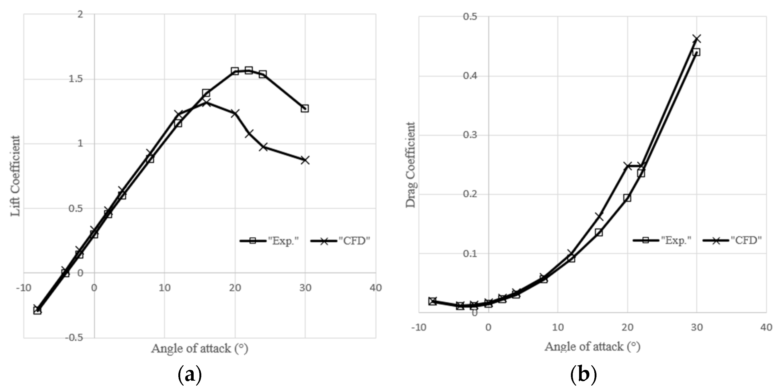
2.4. Validation

The mathematical model was validated using the wind tunnel testing on NACA airfoils from the literature [23]. The study under consideration comprises experiments conducted in a wind tunnel with varied density. Through the variable-density wind tunnel, experimental data can be obtained for high-Reynolds-number flows. For data validation, CFD analysis was performed with a 3D single-wing geometry with the NACA 4415 airfoil. At a 20.7 atm, analyses were conducted at 21.1836 m/s using a Reynolds number of 3,110,000. The turbulence model SST k-ω (with wall function) was used to model eddy viscosity.

In order to establish the boundary layer’s mesh structure, the value of y⁺ was intended to be 10. This parameter is a dimensionless value and is used to determine the height of the first layer of the mesh elements to be created for the boundary layer. Depending on the dimensionless y⁺, the first layer thickness y is defined as [24]

$$y={\displaystyle \frac{u_{\tau }{y}^{+}}{v}},$$

(5)

where v is the kinematic viscosity and u_t is the friction velocity at the closest wall, defined as [24]

$$u_{\tau }=\sqrt{{\displaystyle \frac{{\tau }_{\omega }}{\rho }}},$$

(6)

where ρ is the density at the wall and τω is the wall shear stress, calculated by [18]

$${\tau }_{\omega }={\displaystyle \frac{\rho C_f{V}^2}{2}},$$

(7)

where V is the velocity and C_f is the skin friction coefficient, calculated by [25]

$$C_f={\displaystyle \frac{0.027}{{Re}^{1/7}}},$$

(8)

In order to achieve the goal of y⁺ = 10, a boundary layer mesh structure consisting of 20 layers with 0.01 mm height for the first layer’s elements was constructed. Figure 3 depicts the boundary layer mesh structure.

The experiments of the literature research were conducted at different angles of attack, and the analyses of the present study were carried out accordingly. A comparison of the experimental study’s data and the CFD analysis’s resultant data is presented in Figure 4. The experimental results and the mathematical model diverge at angles of attack of 12° and above. At small angles of attack, the results do, however, appear to accord. In the swarm motion analysis, which is the main subject of the present study, small angles of attack were used, corresponding to high performance, so the mathematical model is suitable for the analysis of small angles of attack.

2.5. Aerodynamic Analysis of Single UAV

The analysis employed the MALE-type UAV geometry with the NACA 4415 airfoil at various angles of attack for a single vehicle. Determining the proper angle of attack for cruise and the aerodynamic effect area of the air flow behind the vehicle are two goals of the analysis using a single UAV.

The model’s sizing parameters, which are obtained from the real model, are listed in

Table 1. Geometric parameters.

Parameter	Value
Wingspan	12 m
Length	6.5 m
Chord length (mean)	0.78 m
Height	1.6 m
Area	9.34 m2

[26]. The height value was taken according to the simplified geometry with the landing gear removed. Similarly, flight parameters were obtained according to the operational altitude value taken from the real model [25]. The flight parameters are shown in

Table 2. Flight parameters in cruise.

Parameter	Value
Altitude	5500 m
Density	0.6975 kg/m3
Viscosity	1.6115 × 10−5 kg/(m·s)
Velocity	36.01 m/s
Re	1,215,714.58

. According to these parameters, within the validated numerical method, the first layer thickness was calculated as 0.15 mm with Equation (5) when y⁺ = 10 was targeted.

The analysis’s findings indicate that the 4–6° angle of attack range corresponds to a high C_L/C_D ratio, an aerodynamic performance metric. A value chosen from this range was likewise subjected to close flight investigation. The performance curve is shown in Figure 5.

The analysis of a single-UAV analysis led to an investigation into the manner in which a vehicle interacts with its surroundings. This results in the formation of a downwash area behind the UAV. In a similar manner, an upwash is formed at the level of the wings. The distances at which close flight analyses should be conducted were established by identifying the regions in question.

A pressure difference between the upper and lower surfaces of an aircraft’s wing is created when it is flying at an angle of attack and a certain speed. This causes the airflow on the lower surface on the wing to roll over the upper surface, creating an inward curling vortex from the wingtip, which is called wingtip vortex. The entire airplane creates two wake vortex zones that are a specific width downstream, creating an outside upwash flow and a downwash flow between the two wake vortex cores. The schematic diagram is displayed in Figure 6, with the plane that provides it one UAV length behind the UAV. This diagram, which shows the variation in the y component of the velocity in the vertical direction, identifies the upwash and downwash areas behind the UAV.

3. Aerodynamic Analysis of the Close-Formation Flight for Two UAVs

The analysis performed on the UAV shows that there is a small variation in the aerodynamic impact over different longitudinal distances. Additionally, Munk’s theorem [27] and related research in the literature [12,13] are compatible with this approach. Therefore, this study only investigates the aerodynamic effects between UAVs, emphasizing only the lateral and vertical distances. Like the diagram in Figure 6, the distribution of the y components of the velocity is shown in Figure 7 over planes at different distances in the rear region of the UAV. With this visualization, it can be seen that the downwash and upwash areas and the values in these areas do not vary much in the longitudinal distance.

3.1. Formation Sequences

The study around the model of the close-formation flight of two UAVs is depicted in Figure 8. The domain where the CFD analyses were performed is box-shaped and its dimensions are height 3.85b (approximately 28 times the UAV height), length 9.5b (approximately 17.5 times the UAV length), and width 5b. There is one UAV positioned in the front, while another UAV trails behind. Both UAVs have matched flying wing configurations and an angle of attack of 5°. The figure illustrates the formation and its coordinate system. In this system, the longitudinal range is represented by the x-axis, the lateral range by the y-axis, and the vertical range inside the formation by the z-axis. Thus, ∆x, ∆y, and ∆z were, respectively, longitudinal, lateral, and vertical distances, as shown in Figure 8.

The wingspan of the UAV is represented by b. The numerical calculation arrangement is displayed in Figure 9 and Figure 10, where the trailing UAV is positioned at 1b in the longitudinal direction behind the leading aircraft. The lateral spacing, changed from 0.625b to 1.5b, was taken as the boundary and analyzed, but the distance 1.375b, the distance before the boundary, was not analyzed in order to reduce the number of analyses. The vertical spacing was changed from −0.266b to 0.266b with an interval of 0.133b, which is the ratio of the UAV height to the wingspan (b), as shown in Figure 10. Thirty-five analyses were performed with a close-formation flight sequence consisting of five vertical locations and seven lateral locations, with a single longitudinal location.

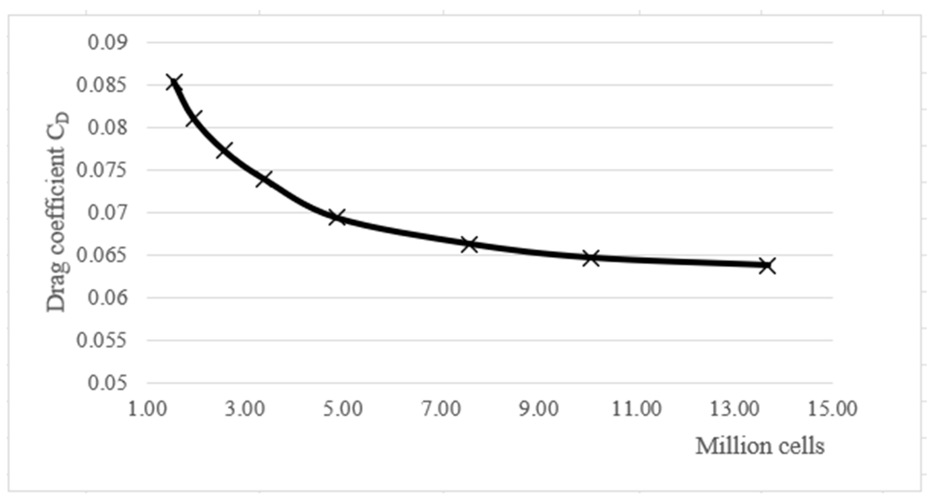
3.2. Mesh Independence

Although the mathematical model has been validated in Section 2.4, the study would be strengthened by performing a mesh independence analysis, especially in the context of determining the appropriate element size. To this end, a mesh independence study was carried out for the two-UAV model. The distances between the two UAVs within the domain in the mesh independence analysis were as follows: ∆x = 26 m, ∆y = 6.4 m, and ∆z = 18 m. The angle of attack in the analyses was chosen to be 6° and the drag coefficient C_D was examined as a parameter for mesh independence. As a result of the analysis, the change in the C_D value of the following UAV, depending on the number of mesh elements, is shown in Figure 11. When the graph is analyzed, it is seen that the C_D curve does not change significantly after 7 million elements. Thus, the number of elements in the analysis for the aerodynamic interaction of swarm UAVs was determined as approximately 7 million.

According to the ANSYS quality standards, the average skewness was 0.03 and the average orthogonal quality was 0.96, which should be sufficient. It was decided that the mesh values were acceptable [18]. The mosaic mesh distribution between the two UAVs is shown in Figure 12. For each analysis, the number of mesh elements and the quality values will vary as the UAV models will be in different positions within the domain. However, since the domain size and UAV model geometry do not change, the change in these values will be acceptably small.

4. Results and Discussion

Thirty-five analyses were carried out as part of the study.

Table 3. UAV’s positions in the analysis and analysis numbers.

∆z	∆y = 3.2 m	∆y = 1.6 m	∆y = 0 m	∆y = −1.6 m	∆y = −3.2 m
18 m	Analysis 1	Analysis 2	Analysis 3	Analysis 4	Analysis 5
15 m	Analysis 6	Analysis 7	Analysis 8	Analysis 9	Analysis 10
12 m	Analysis 11	Analysis 12	Analysis 13	Analysis 14	Analysis 15
9 m	Analysis 16	Analysis 17	Analysis 18	Analysis 19	Analysis 20
10.5 m	Analysis 21	Analysis 22	Analysis 23	Analysis 24	Analysis 25
7.5 m	Analysis 26	Analysis 27	Analysis 28	Analysis 29	Analysis 30
13.5 m	Analysis 31	Analysis 32	Analysis 33	Analysis 34	Analysis 35

displays the UAV positions that were involved in the thirty-five analyses conducted for the study. All analyses were performed longitudinally at a distance of ∆x = 13 m.

The trailing UAV’s lift coefficients (C_L) that are results of the aerodynamic effect are plotted against the lateral distances between the UAVs in Figure 13. In this figure, different vertical distances are shown with different curves. It is evident that ∆y = 0 m always has the maximum C_L value for whatever the lateral distance position is. In other words, regardless of the lateral distance, when the leading UAV and the trailing UAV fly at the same altitude, the trailing UAV has the maximum lift coefficient. The ∆y = 0.133b and ∆y = −0.133b curves represent the positions where the trailing UAV flies one vehicle height higher and lower than the leading UAV (0.133b = 1.6 m, where b is the wingspan). These two curves present the same values, except for the points ∆z = 12 m and ∆z = 13.5 m. Similarly, the ∆y = 0.266b and ∆y = −0.266b curves at the positions where the trailing UAV flies two vehicle heights higher and lower than the leading UAV have very close values. However, these curves have lower C_L values than the ∆y = 0.133b and ∆y = −0.133b curves. In the same altitude plane (∆y = 0 m) with maximum C_L value, it was determined that the C_L value decreased by similar amounts when diverging up or down. So, the C_L values of the trailing UAV show a symmetrical value change when the same altitude plane is considered as the plane of symmetry, which is consistent with the schematic diagram in Figure 6. In close-formation flight, where the lateral distance between the two UAVs is 1.5 times the wingspan (∆z = 18 m), the C_L values are slightly different for different vertical distances. For these positions in the context of C_L, it can be said that the aerodynamic effect between the two UAVs is significantly reduced.

The drag coefficients of the trailing UAV for different lateral distances are shown in Figure 14. The C_D values for different vertical distances are presented by different curves, with the lateral distance values being variable. At ∆z = 15 m and ∆z = 18 m, the change in vertical distance becomes insignificant; i.e., the C_D values are approximately the same. For other lateral distance values, the ∆z = 0 m curve has the lowest C_D values. Conversely, ∆z = 0.266b and ∆z = −0.266b curves have the highest C_D values. These two curves contain approximately the same values. Similarly, the ∆z = 0.133b and ∆z = −0.133b curves have approximately the same results for the same lateral distances. As in the C_L plot, C_D values around the same altitude plane (∆z = 0 m) show a symmetrical distribution in the upward and downward direction for different vertical distances.

The optimum position, where the trailing UAC can achieve the greatest aerodynamic improvement, is identified as the position of the maximum lift-to-drag ratio of the trailing UAV during close-formation flight. The maximum aerodynamic performance curve is generated when two UAVs fly at the same altitude in comparison to other vertical distances, as shown in Figure 15. A symmetrical representation with respect to the axis at the same altitude is formed by the values at various vertical distances. In other words, the outcomes of the analyses with ∆y = 0.133b and ∆y = −0.133b concur. The results of the analyses with ∆y = 0.266b and ∆y = −0.266b likewise coincide. The investigation using horizontal distances shows that the maximum aerodynamic performance occurs at ∆z = 0.875b and ∆z = 1b.

The performance improvement histogram for the 35 analyses is displayed in Figure 16, in which the analysis numbers are as in Table 3. Based on the improvement in the trailing UAV’s aerodynamic performance over the leading UAV’s aerodynamic performance in the same analysis, this histogram was created. The ∆z = 0.875b and ∆z = 1b positions with the best performances are the 13th and 23rd analyses, respectively. In both analyses, ∆y = 0 m and the performance improvements are 11.43% and 11.56%, respectively. The histogram also shows us that there are performance degradations as in the 26th, 29th, and 30th analyses. These are the analyses of the trailing UAV at a lateral distance ∆z = 0.625b. At this distance, the downwash area behind the lead UAV is now more effective than the upwash area.

5. Conclusions

This paper uses CFD analysis to study the close-formation flight for a MALE class UAV model with fixed wing. Using 3D wing wind tunnel test results, the mathematical model is first validated using data. Next, the region of the aerodynamic effect is examined, and a single UAV is evaluated. The primary focus of the study is the analysis of two UAVs for flights at different positions. The following outcomes of these analyses were attained for the case of a flocked cruise in the V-formation:

(1)

The characteristics in the aerodynamic interaction region of the longitudinal distance behind the UAV do not change greatly.

(2)

Two UAVs flying in close formation should avoid flying inside the wing line to avoid entering the downwash area, as this can have a negative interaction.

(3)

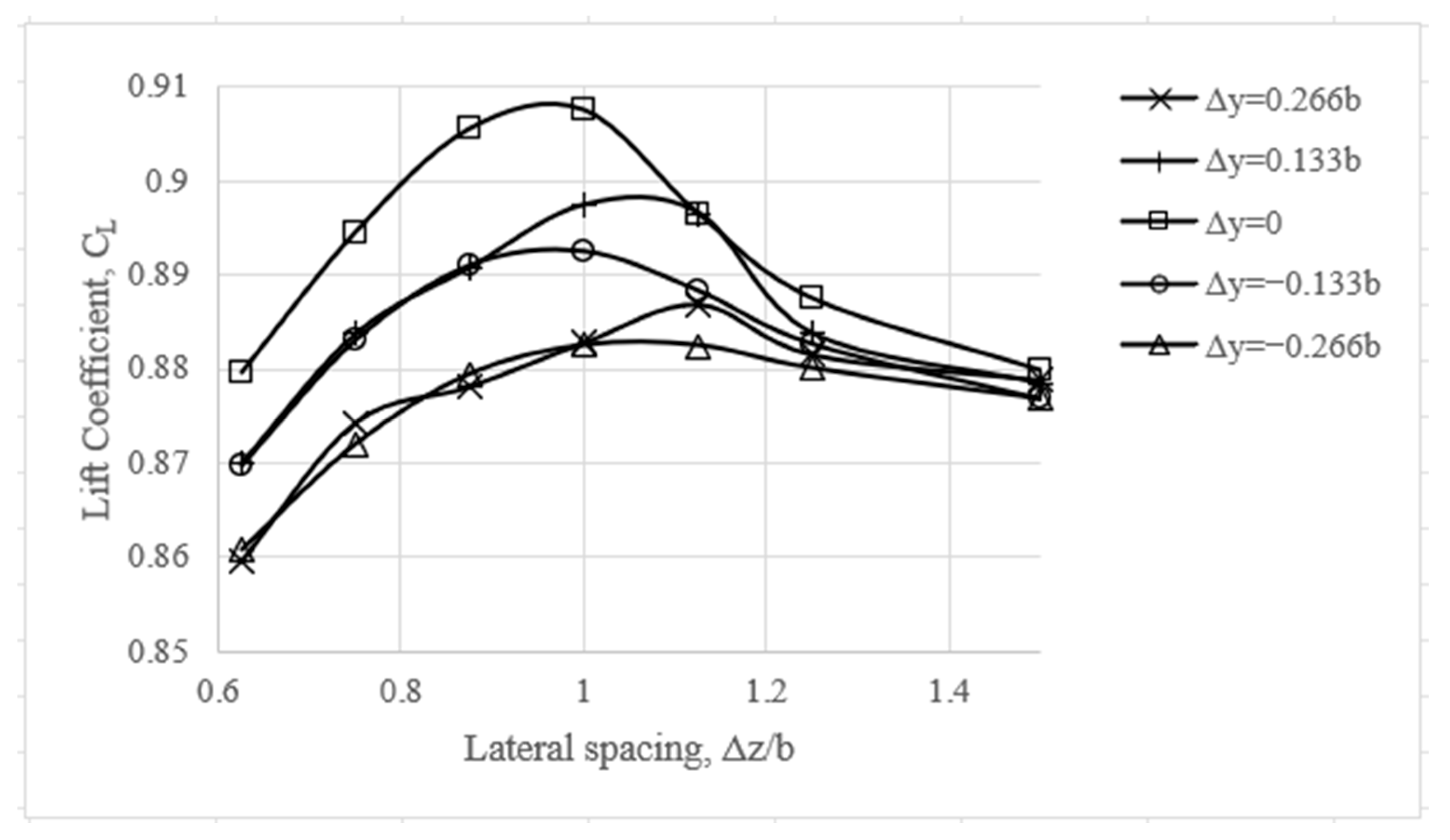
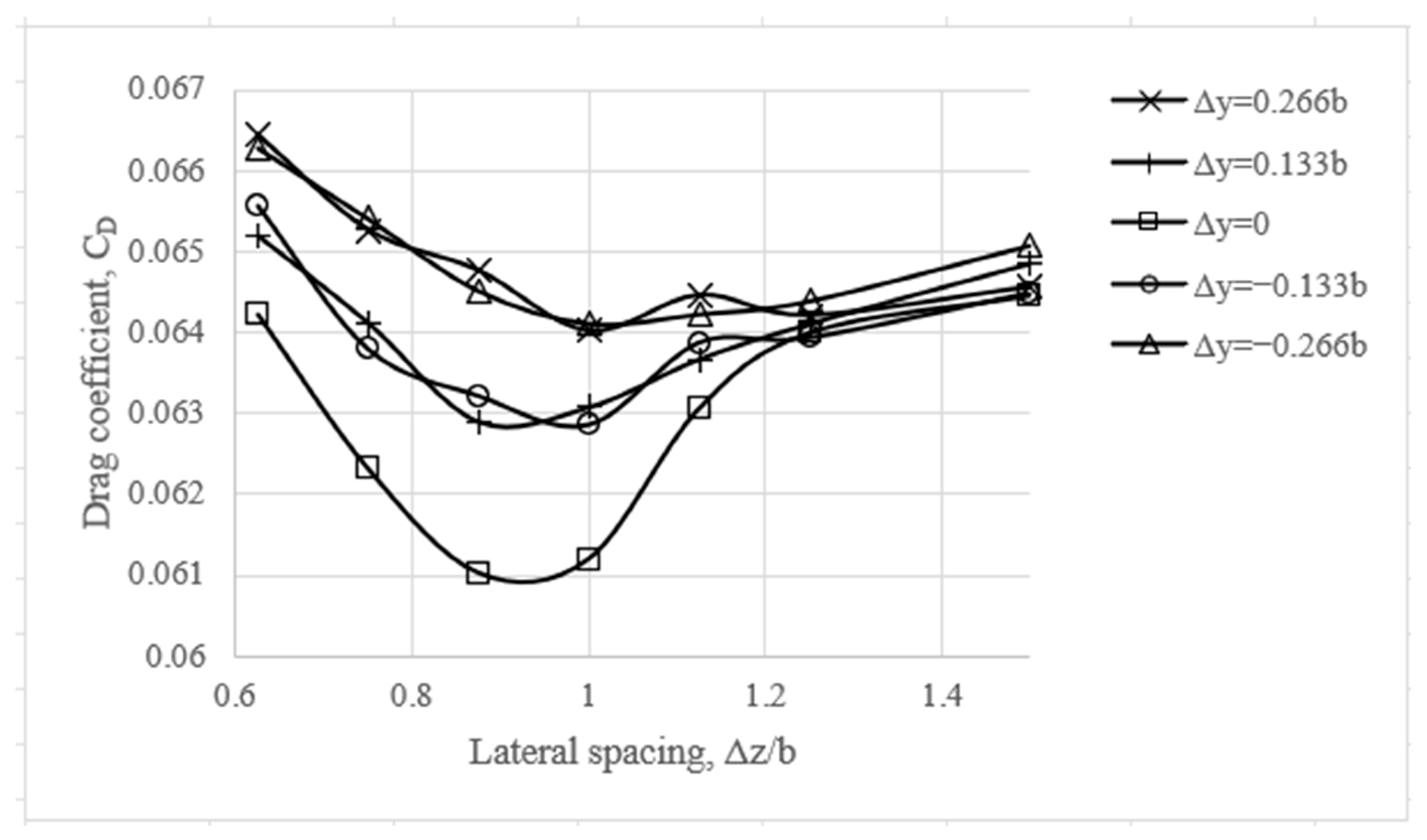
For the most efficient aerodynamic performance in close flight of swarm UAVs, they must fly at the same altitude, i.e., in the same vertical alignment.

(4)

For b wingspan, the most aerodynamically efficient spots for close-formation flight are lateral distances of 0.875b and 1b.

(5)

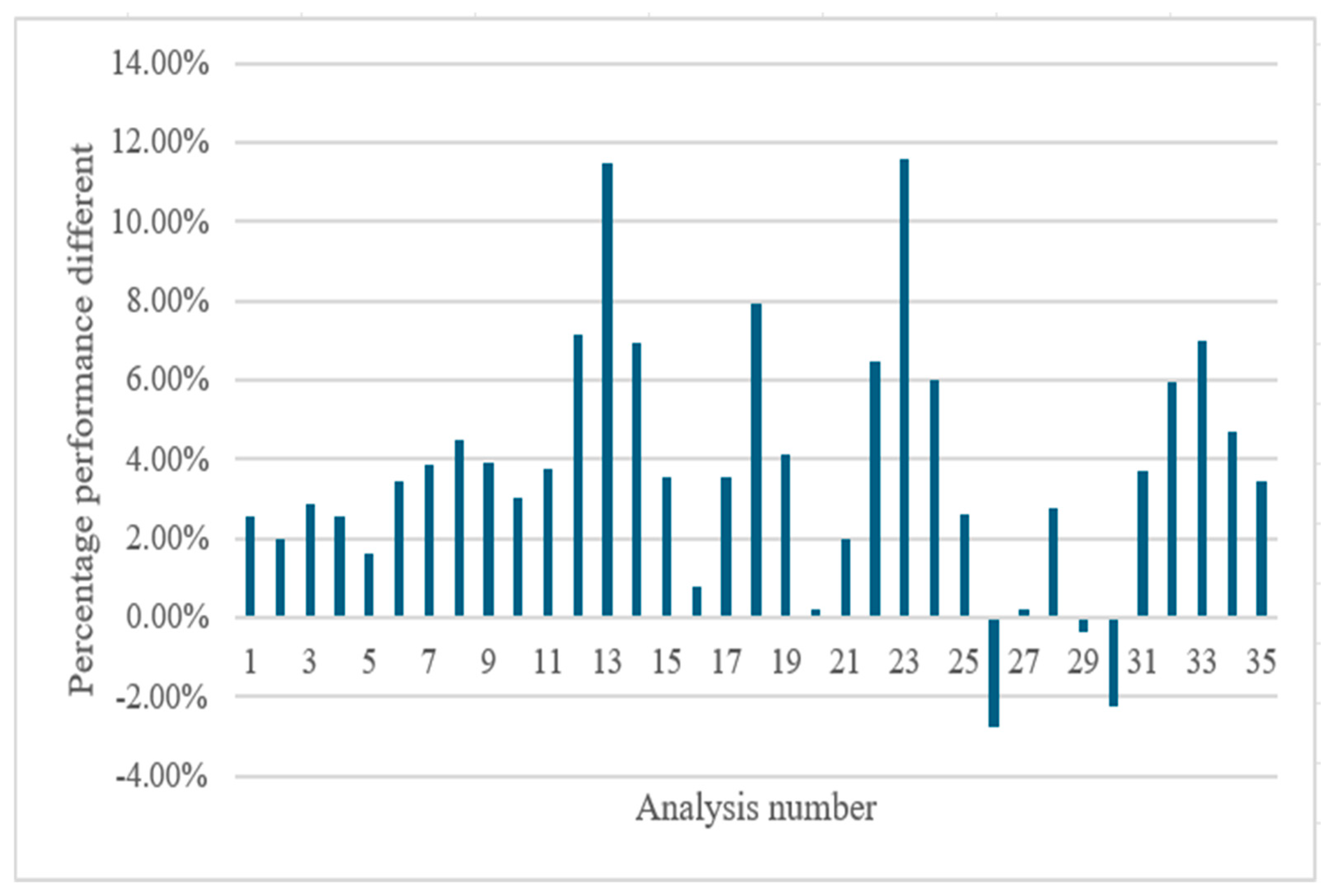
Considering C_L/C_D as an aerodynamic performance parameter, in the most efficient flight positions, the trailing UAV has an efficiency increase of about 11.5% compared to a single flight.

References

- Shao, Z.; Yan, F.; Zhou, Z.; Zhu, X. Path planning for multi-UAV formation Rendezvous based on distributed cooperative particle swarm optimization. Appl. Sci. 2019, 9, 2621. [Google Scholar] [CrossRef]
- Wieselsberger, C. Beitrag zur erklärung des winkelfluges einiger zugvöge. Z. FlugTechnick Mot. 1914, 5, 225–229. [Google Scholar]
- Lissaman, P.B.S.; Schollenberger, C.A. Formation flight of birds. Science 1970, 168, 1003–1005. [Google Scholar] [CrossRef] [PubMed]
- Hansen, J.L.; Cobleigh, B.R. Induced moment effects of formation flight using two F/A-18 aircraft. In Proceedings of the AIAA Atmospheric Flight Mechanics Conference and Exhibit, Monterey, CA, USA, 5–8 August 2002. [Google Scholar]
- Pahle, J.; Berger, D.; Venti, M.; Duggan, C.; Faber, J.; Cardinal, K. An initial flight investigation of formation flight for drag reduction on the C-17 aircraft. In Proceedings of the AIAA Atmospheric Flight Mechanics Conference, Minneapolis, MN, USA, 13–16 August 2012. [Google Scholar]
- Dogan, A.; Venkataramanan, S.; Blake, W. Modeling of aerodynamic coupling between aircraft in close proximity. J. Aircr. 2005, 42, 941–955. [Google Scholar] [CrossRef]
- Singh, D.; Antoniadis, A.F.; Tsoutsanis, P.; Shin, H.; Tsourdos, A.; Mathekga, A.; Jenkins, K.W. A multi-fidelity approach for aerodynamic performance computations of formation flight. Aerospace 2018, 5, 66. [Google Scholar] [CrossRef]
- Yuan, G.; Xia, J.; Duan, H. A continuous modeling method via improved pigeon-inspired optimization for wake vortices in UAVs close formation flight. Aerosp. Sci. Technol. 2021, 120, 107259. [Google Scholar] [CrossRef]
- Blake, W.; Gingras, D.R. Comparison of predicted and measured formation flight interference effects. J. Aircr. 2004, 41, 201–207. [Google Scholar] [CrossRef]
- Trumic, E.; Swamy, K.S. Aerodynamic Performance Analysis of a UAV Using CFD and VLM. Master’s Thesis, Linköping University, Linköping, Sweden, 2021. [Google Scholar]
- Cui, X.; Yu, Y.; Ma, S.; Xiao, Z.; Zhang, L.; Liu, F. Numerical investigation of the aerodynamic interference in 2-aircraft formation flight. J. Phys. Conf. Ser. 2022, 2280, 012017. [Google Scholar] [CrossRef]
- Yang, T.; Zhiyong, L.; Neng, X.; Yan, S.; Jun, L. Optimization of positional parameters of close-formation flight for blended-wing-body configuration. Heliyon 2018, 4, e01019. [Google Scholar] [CrossRef] [PubMed]
- Zhang, D.; Chen, Y.; Dong, X.; Liu, Z.; Zhou, Y. Numerical aerodynamic characteristics analysis of the close formation flight. Math. Probl. Eng. 2018, 2018, 3136519. [Google Scholar] [CrossRef]
- Shin, H.; Antoniadis, A.F.; Tsourdos, A. Parametric study on efficient formation flying for a blended-wing UAV. In Proceedings of the 2017 International Conference on Unmanned Aircraft Systems (ICUAS), Miami, FL, USA, 13–16 June 2017. [Google Scholar]
- Panagiotou, P.; Yakinthos, K. Aerodynamic efficiency and performance enhancement of fixed-wing UAVs. Aerosp. Sci. Technol. 2019, 99, 105575. [Google Scholar] [CrossRef]
- Shunshun, W.; Zheng, G. Design, optimization and application of two-element airfoils for tactical UAV. Adv. Mech. Eng. 2022, 14, 1–14. [Google Scholar] [CrossRef]
- Pastor, L.G.S. Numerical Design and Optimization of a Rescue UAV’s Wing. Bachelor’s Thesis, Universitat Politècnica de València, Valencia, Spain, 2022. [Google Scholar]
- Arabacı, S.K.; Dilbaz, F. Aerodynamic Analysis of Anka UAV and Heron UAV. In Proceedings of the 2nd International Conference on Energy Research, Marmaris, Turkey, 11–13 April 2019. [Google Scholar]
- Zore, K.; Sasanapuri, B.; Parkhi, G.; Varghese, A. ANSYS mosaic poly-hexcore mesh for high-lift aircraft configuration. In Proceedings of the 21st Annual CFD Symposium, Bangalore, India, 8–9 August 2019. [Google Scholar]
- Pezzella, G.; Viviani, A. Aerodynamic Performance Analysis of Three Different Unmanned Re-entry Vehicles. In Advanced UAV Aerodynamics, Flight Stability and Control, 1st ed.; Marquès, P., Da Ronch, A., Eds.; Wiley: Hoboken, NJ, USA, 2017; pp. 49–141. [Google Scholar]
- Aydın, N.; Çalışkan, M.E.; Karagöz, İ. Numerical simulation of flow over NACA 0015 airfoil with different turbulence models. Int. J. Energy Appl. Technol. 2020, 7, 42–49. [Google Scholar] [CrossRef]
- Menter, F.R. Zonal two equation k-ω turbulence models for aerodynamic flows. In Proceedings of the 24th Fluid Dynamics Conference, Orlando, FL, USA, 6–9 July 1993. [Google Scholar]
- Jacobs, E.N.; Ward, K.E.; Pinkerton, R.M. The Characteristics of 78 Related Airfoil Sections from Tests in the Variable-Density Wind Tunnel; Report No. 460; National Advisory Committee for Aeronautics: Washington, DC, USA, 1935. [Google Scholar]
- Steenwijk, B.; Druetta, P. Numerical study of turbulent flows oner a NACA 0012 airfoil: Insights into its performance and the addition of a slotted flap. Appl. Sci. 2023, 17, 7890. [Google Scholar] [CrossRef]
- Çengel, Y.; Cimbala, J.M. Akışkanlar Mekaniği, 1st ed.; Güven Bilimsel: İzmir, Türkiye, 2008. [Google Scholar]
- Baykar. Available online: https://baykartech.com/tr/uav/bayraktar-tb2/ (accessed on 13 May 2024).
- Munk, M.M. The Minimum Induced Drag of Aerofoils; Report No. 121; National Advisory Committee for Aeronautics: Washington, DC, USA, 1923. [Google Scholar]