Dynamic Modeling and Optimization of Tension Distribution for a Cable-Driven Parallel Robot

Abstract

Cable-driven parallel robots (CDPRs) have been gaining much attention due to their many advantages over traditional parallel robots or serial robots, such as their markedly large workspace and lightweight design. However, one of the main issues that needs to be urgently solved is the tension in the distribution of CDPRs due to two reasons. The first is that a cable can only be stretched but not compressed, and the other is the redundancy of the parallel robot. To address the problem, an optimization method for tension distribution is proposed in the paper. The structural design of the parallel robot is first discussed. The dynamics model of the parallel robot is established by the Newton–Euler method. Based on the minimum variance of cables’ tension, an optimization method of tension distribution is presented for the parallel robot. Furthermore, the tension extreme average term is introduced in the optimization method, and the firefly algorithm is applied to obtain the optimal solution for tension distribution. Finally, the proposed approach is tested in the simulation case where the end-effector of the robot moves in a circular motion. Simulation results demonstrate that the uniformity and continuity of tension are both outstanding for the proposed method. In contrast with traditional solving methods, the efficiency of this method is largely improved.

1. Introduction

Cable-driven parallel robots have many advantages over other robots driven by traditional styles such as mechanical, hydraulic, or pneumatic modes. This is because traditional-driven styles have the same defect, which is that the motion range of the end-effector is significantly limited [1]. In contrast, the CDPR allows the end-effector to move rapidly in a large space due to its drive characteristics [2,3,4]. By adjusting the cable tension, the cable-driven parallel robot has the advantages of high load capacity, broad working space, and low motion inertia [5,6]. Therefore, it is widely used in many fields, such as industrial lifting [7], medical rehabilitation [8,9], tactile interaction [10], and 3D printing [11,12].

Scholars were committed to studying the related issues of the cable tension distribution algorithm for cable-driven parallel robots. Bin Zhang proposed a new two-loop dynamic control scheme, which introduced the parallel two-loop tracking strategy and provided a more compatible scheme but did not take into account the real-time performance of the cable tension method [13]. Wang Yan-lin studied the mechanical characteristics of a cable-driven lower limb rehabilitation robot (CDLR). The mechanical properties of cable-driven lower limb rehabilitation robot (CDLR) were designed and studied. [14]. Song Da used a non-iterative, two-degree-of-freedom-driven redundant CDPR real-time cable tension distribution algorithm to solve the cable tension [15]. Based on the feasible polygon of CDPR and its stiffness matrix, Picard selected a set of allowable cable tensions to minimize the movement of the platform displacement [16]. Adel Ameri employed a new method for the distribution of positive tension in cable-driven parallel robots. In the method, a nonlinear disturbance observer was introduced to eliminate kinematic uncertainties caused by redundant resolution [17].

However, the above studies only focused on analyzing the tension calculation, and there is little research on tension distribution optimization. Additionally, some tension calculation methods had certain defects, such as discontinuity. In order to optimize the tension distribution of a planar parallel robot driven by four cables, Dao took advantage of the quadratic programming algorithm and the dynamic model to deal with the optimization problem [18]. Chen Yizong established a system dynamics model considering wave excitation to improve the positioning accuracy and anti-interference ability of the moving platform with the end-effector installed. Further, he studied the controllable workspace and cable tension optimization algorithms [19]. Kieu has developed an improved kinematic equation that takes into account the nonlinear tension of the cable based on a dynamic mechanical analysis (DMA) method to determine the optimal cable tension at each position of the end actuator [20]. CaoSheng provides a tension function containing a hyperbolic tangent function, which can simultaneously implement the necessary wrench and the appropriate tension distribution and manage the tension distribution optimization [21]. These four studies only analyzed the tension optimization of the cable-driven parallel structure with four cables and three degrees of freedom but did not optimize the tension of the cable-driven parallel mechanism with more than four degrees of freedom and did not consider the influence of system stiffness on cable tension optimization. Pott presents an algorithm that can be used to calculate the cable tension distribution of a cable-driven parallel robot with arbitrary redundancy and gives the formula for the cable tension distribution in the form of an analytic solution. However, the algorithm may not be solved in some cases [22,23]. Gouttefarde et al. proposed a cable force distribution of an n-DOF parallel robot driven by n + 2 cables. Taking a 6-DOF 8-cable-driven parallel robot system as an example, by introducing two random variables, the cable tension was expressed as the equation of these two random variables. The author further analyzes the equations of these two random variables and finds that their geometric meaning is eight pairs of intersecting parallel lines, and the feasible solution of the cable tension is the common area algorithm of these eight groups of parallel lines. However, due to the large randomness of the initial point selection, the calculation time of the whole algorithm is also uncertain [24]. Lim et al. used the modified gradient projection method to optimize and solve the cable tension to obtain the tension required by the cable tension index. However, the solution speed and the continuity of the optimal solution need to be improved [25]. Using five gradient-based particle optimization heuristics, Parque optimizes the tension distribution problem, where the use of a cost function based on the sum of squares of forces results in a feasible, but not always smooth, force distribution [26].

In view of this, the improved minimum variance method is used to solve the problem of insufficient tension, stiffness, and discontinuity of the cable. This paper mainly studies the cable-driven parallel robot, especially the cable-driven parallel mechanism with redundant constraints. Based on the Newton–Euler method, the system dynamics model of cable-driven parallel robots is established. By introducing constraint conditions, the firefly algorithm is used to solve the optimal solution of tension distribution.

The remainder of this paper is as follows: Section 2 introduces the mechanical structure of the cable-driven parallel robot. Section 3 establishes the dynamic model. In Section 4, a detailed solution for cable tension distribution is presented. Section 5 includes simulation studies for the traditional method and the proposed method. Section 6 includes the conclusion and discussion, respectively.

2. Design of Parallel Robot

2.1. Constraint Classification of Parallel Mechanism

The current parallel mechanism popular in the market and research institutes makes a deeper analysis and summary of the mathematical relationship between the cable freedom degree $n$ and the cable number $y$ and finally divides the cable drive parallel mechanism into three categories [27]. For the first type of unconstrained cable drive parallel mechanism, the number of driving cables is less than the number of degrees of freedom. The second type is the fully constrained cable drive parallel mechanism, whose driving cable numbers are equal to the number of degrees of freedom. The last type is an overconstrained cable drive parallel mechanism, and the number of cable drives is greater than the number of degrees of freedom. The total is shown in

Table 1. The total of machine technical parameters.

Constrained Type	Establishment Condition	Example
Incompletely restrained positioning mechanisms	$y<n+1$	$y=6;n=6$
Completely restrained positioning mechanisms	$y=n+1$	$y=7;n=6$
Redundantly restrained positioning mechanisms	$y>n+1$	$y=8;n=6$

.

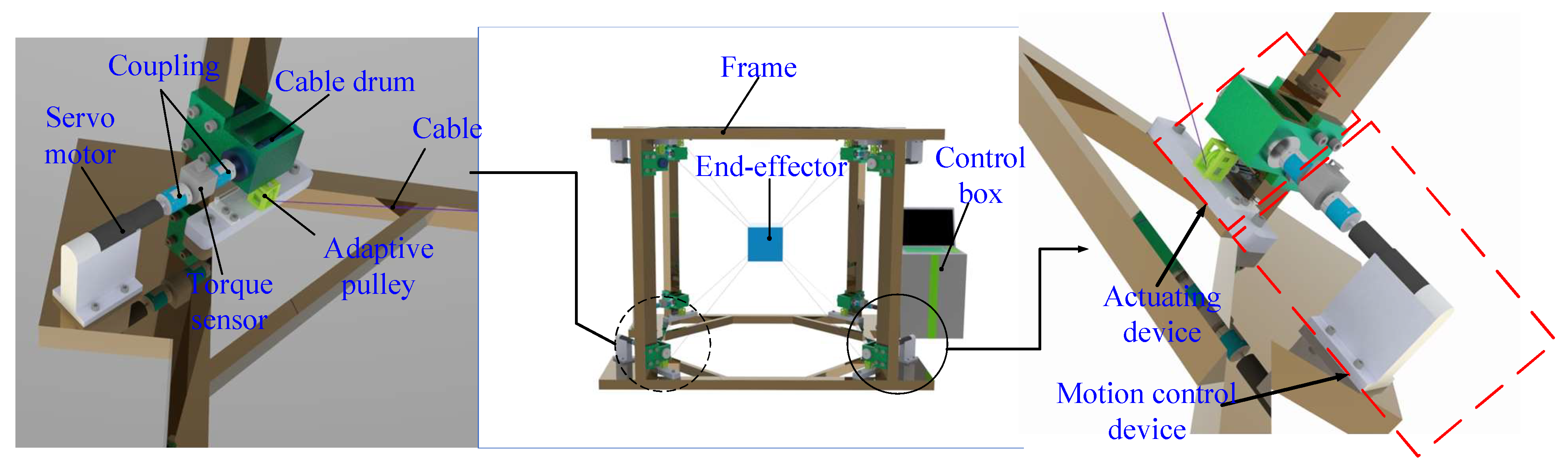
2.2. Overall Structural Design

The structure model of the cable-driven parallel robot, which consists of a frame, eight cables driven by actuator systems, a control box, and an end-effector, is shown in Figure 1. Each actuator system is composed of a servo motor, coupling, cable drum, and adaptive pulley. Servo motors are fixed at the eight vertices of the frame. The output shaft of a servo motor is connected to a cable drum by couplings. The cable drum is driven by a servo motor so that the cable around the cable drum can be pulled and released. The adaptive pulley, which is an important part of the actuator system, can make the cable adapt to the direction of the end effector extremely quickly, which guarantees the translation or rotation of the end effector effectively. The overall structural design is also divided into a frame, drive device, motion control device, and end effector, as shown in Figure 2. The structural and technical parameters of the cable-driven parallel robot are shown in

Table 2. Complete machine technical parameters.

Technical Parameters	Value
Overall size (L·W·H)/(mm·mm·mm)	1000 × 1000 × 1000
Overall machine mass/(kg)	30.6
Drive stepper motor torque/(N·M)	1.91
Cable drum diameter/(cm)	8

.

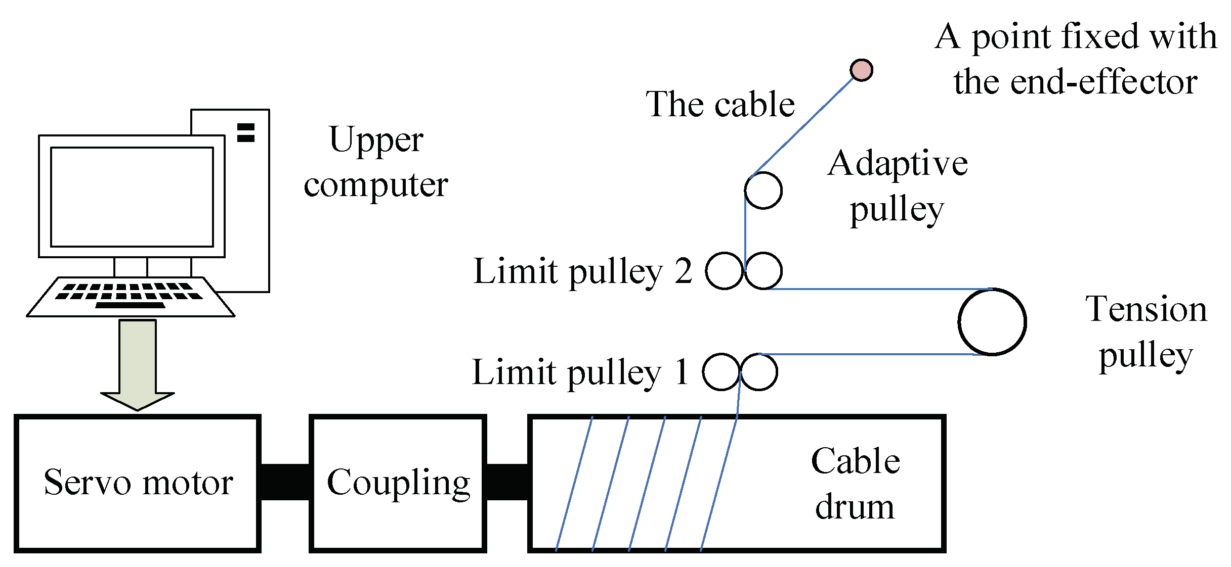
2.3. Principle of Working for the Robot

As shown in Figure 3, this is the working principle of the cable-driven parallel robot. The servo motor starts to work when it receives the signal sent by an upper computer, which is in the control box, and the cable drum will rotate with the servo motor at the same speed. Therefore, the cable could be released and pulled by the rotation of the cable drum. The attitude of this cable is fixed by Limit Pulley 1 first, and then the cable is tensioned by a tension pulley. Moreover, the other pulley, named Limit Pulley 2, is used to fix the attitude of the cable. In order to control the direction of the cable much better, an adaptive pulley is mounted behind Limit Pulley 2. Finally, the cable is fixed to the end-effector of the robot after the cable comes around the adaptive pulley. And the movement of the end-effector can be implemented by releasing and pulling cables.

3. Dynamics Model of the Robot

The dynamics model is the basis of trajectory tracking control. The accuracy of the dynamics model directly affects the precision of the trajectory tracking of the cable-driven parallel robot. Therefore, the dynamics modeling of the parallel robot is established in this section.

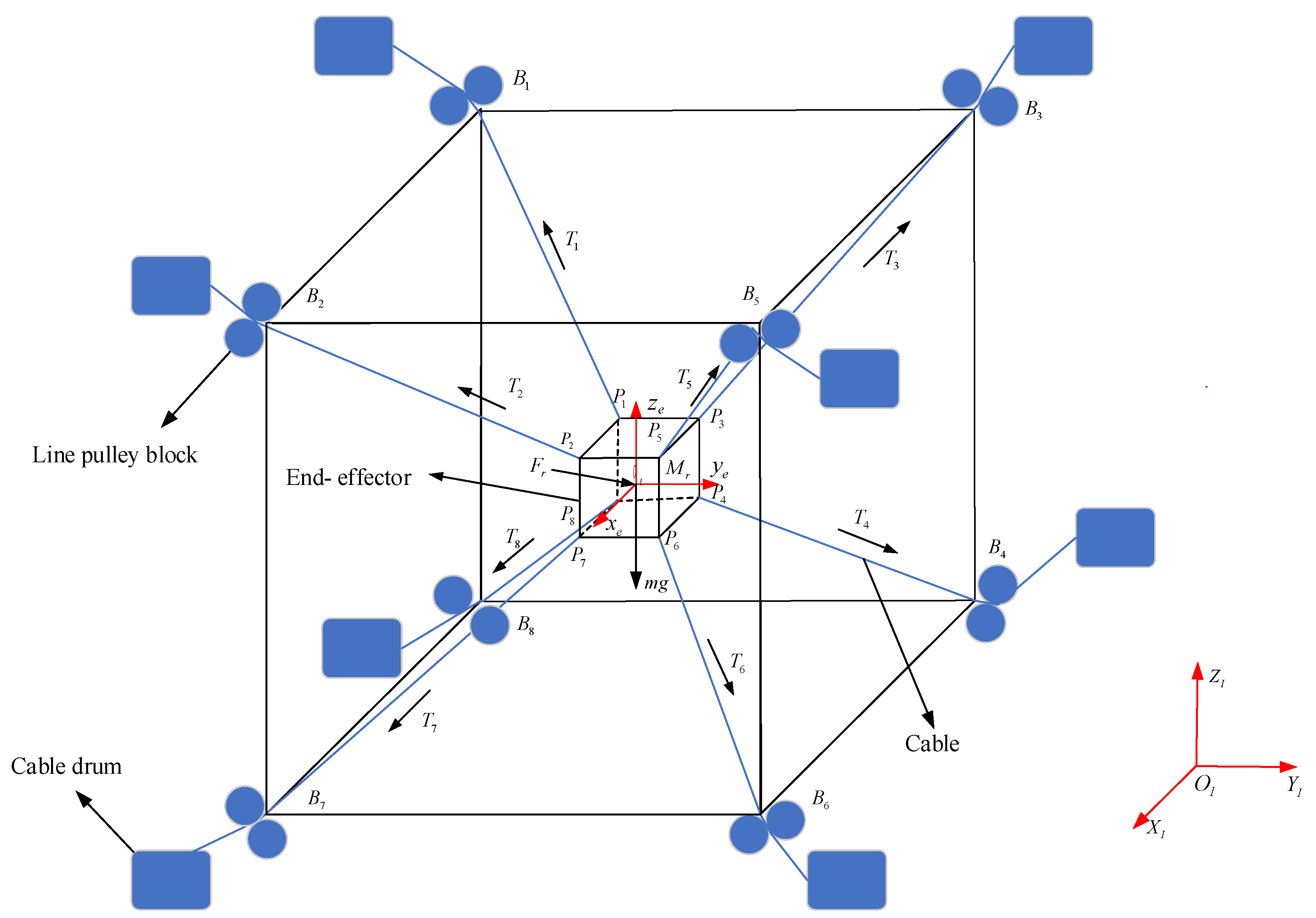
3.1. Force Analysis of the End-Effector

In fact, since the movement of the end-effector is implemented by releasing and pulling cables, there is a tension that acts on the end-effector for each cable. Additionally, the end-effector is also affected by gravity. The end-effector’s force analysis is shown in the Figure 4. Points B₁~B₈ represent the vertexes of the frame, and Points P₁~P₈ are the vertexes of the end-effector. T_i (i = 1, 2,…,8) is the tension of the ith cable between Point B_i and P_i. The coordinate system o_e − x_ey_ez_e is fixed on the center of the end-effector. The coordinate system O_I − X_IY_IZ_I is an inertial system denoted by ∑_I. For the convenience of dynamics modeling, two assumptions are as follows:

(a)

The weight of the cable in the coordinate system o_e − x_ey_ez_e is fixed on the center of the end-effector. The coordinate system O_I − X_IY_IZ_I is an inertial system denoted by ∑_I. For the convenience of dynamics modeling, two assumptions are as follows: is not considered in dynamics modeling due to the tiny mass of the cable;

(b)

The cable is an ideal, flexible body that does bending or shearing force. Based on the above assumptions and the Newton–Euler Equation, the dynamics model of the end-effector is given as follows:

$$\left\{\begin{array}{l}m\dot{v}+G_e={\displaystyle \sum _{i=1}^8{T}_i+F_r}\\ I\dot{\omega }+\omega \times I\omega ={\displaystyle \sum _{i=1}^8{r}_i\times T_i+M_r}\end{array}\right.$$

(1)

where m is the mass of the end effector. v = [v_x, v_y, v_z]^T denotes the linear velocity of the end-effector. G_e is the gravity of the end-effector. I is the inertial matrix, and ω represents the angular velocity. r_i is the position vector from o_i to P_i. F_r and M_r represent external force and torque acting as the end-effector, respectively. For ease of analysis and processing, the Equation (1) could be rewritten as follows.:

$$M\dot{x}+Vx+G=JT+E_r$$

(2)

where M, V, and G are the inertia term, Coriolis term, and gravity term of the end-effector. J, T, and E_r represent the generalized moment arm matrix, tension matrix, and generalized external force/torque matrix. x is the generalized velocity of the end-effector. The specific expression of them is as follows:

$$M=\left[\begin{array}{cc}m{E}_{3\times 3}& {\mathbf{0}}_{3\times 3}\\ {\mathbf{0}}_{3\times 3}& I\end{array}\right]\in {ℝ}^{6\times 6},V=\left[\begin{array}{cc}{\mathbf{0}}_{3\times 3}& {\mathbf{0}}_{3\times 3}\\ {\mathbf{0}}_{3\times 3}& -{\left(I\omega \right)}^{\times }\end{array}\right]\in {ℝ}^{6\times 6},G=\left[\begin{array}{c}{G}_e\\ {\mathbf{0}}_{3\times 3}\end{array}\right]\in {ℝ}^{6\times 1}$$

(3)

$$J=\left[\begin{array}{cccccccc}{\mathbf{0}}_{3\times 3}& {\mathbf{0}}_{3\times 3}& {\mathbf{0}}_{3\times 3}& {\mathbf{0}}_{3\times 3}& {\mathbf{0}}_{3\times 3}& {\mathbf{0}}_{3\times 3}& {\mathbf{0}}_{3\times 3}& {\mathbf{0}}_{3\times 3}\\ r_1^{\times }& r_2^{\times }& r_3^{\times }& r_4^{\times }& r_5^{\times }& r_6^{\times }& r_7^{\times }& r_8^{\times }\end{array}\right]\in {ℝ}^{6\times 24}$$

(4)

$$T={\left[\begin{array}{cccccccc}{T}_1^{{\rm T}}& T_2^{{\rm T}}& T_3^{{\rm T}}& T_4^{{\rm T}}& T_5^{{\rm T}}& T_6^{{\rm T}}& T_7^{{\rm T}}& T_8^{{\rm T}}\end{array}\right]}^{{\rm T}}\in {ℝ}^{24\times 1}$$

(5)

$$E_r=\left[\begin{array}{c}{F}_r\\ M_r\end{array}\right]\in {ℝ}^{6\times 1}$$

(6)

$$x=\left[\begin{array}{c}v\\ \omega \end{array}\right]\in {ℝ}^{6\times 1},\dot{x}=\left[\begin{array}{c}\dot{v}\\ \dot{\omega }\end{array}\right]\in {ℝ}^{6\times 1}$$

(7)

$E_{3\times 3}$ and ${\mathbf{0}}_{3\times 3}$ are unit matrix and zero matrix. $r_i^{\times }$ is the skew-symmetric matrix of $r_i$, i.e.,

$$\mathrm{if} r_i=\left[\begin{array}{ccc}{r}_{ix}& r_{iy}& r_{iz}\end{array}\right], \mathrm{then} r_i^{\times }=\left[\begin{array}{ccc}0& -r_{iz}& r_{iy}\\ r_{iz}& 0& -r_{ix}\\ -r_{iy}& r_{ix}& 0\end{array}\right]$$

(8)

3.2. The Driving Device’s Dynamics Model

The generation of a cable’s tension is owing to the drag of the cable drum driven by the motor, so it is necessary to establish its dynamics model. Similarly, according to the Newton–Euler method, the dynamic model of the ith cable drum is as follows:

$$J_{d_i}{\ddot{\gamma }}_{d_i}+V_{d_i}{\dot{\gamma }}_{d_i}+r_{d_i}{T}_i={\tau }_{d_i},(i=1,2,\dots ,8)$$

(9)

where $J_{d_i}$ and $V_{d_i}$ are the cable drum’s inertia and viscosity damping coefficient. The radius of the cable drum denotes $r_{d_i}$. ${\tau }_{d_i}$ is the applied moment generated by the servo motor. ${\gamma }_{d_i}$ represent the rotation angle of the cable drum and it can be obtained as follows:

$${\gamma }_{d_i}=r_{d_i}^{-1}\left(l_i(k)-l_i(k-1)\right)$$

(10)

$l_i(k)$ and $l_i(k-1)$ are the length of the ith cable at the current time and last time, respectively. Based on Equation (9), the tension’s value of the ith cable is calculated by

$$T_i=r_{d_i}^{-1}\left({\tau }_{d_i}-J_{d_i}{\ddot{\gamma }}_{d_i}-V_{d_i}{\dot{\gamma }}_{d_i}\right),(i=1,2,\dots ,8)$$

(11)

Because of $T_i=‖T_i‖$, $T_i$ can be rewritten as $T_i=T_i{u}_i$. $u_i$ is the unit directional vector of $T_i$. According to Equation (5), it can be yielded as follows:

$$\begin{array}{l}T={\left[\begin{array}{cccccccc}{T}_1^{{\rm T}}& T_2^{{\rm T}}& T_3^{{\rm T}}& T_4^{{\rm T}}& T_5^{{\rm T}}& T_6^{{\rm T}}& T_7^{{\rm T}}& T_8^{{\rm T}}\end{array}\right]}^{{\rm T}}\\ =\left[\begin{array}{cccc}{T}_1{E}_{3\times 3}& & & \\ & T_2{E}_{3\times 3}& & \\ & & \ddots & \\ & & & T_8{E}_{3\times 3}\end{array}\right]\left[\begin{array}{c}{u}_1\\ u_2\\ ⋮\\ u_8\end{array}\right]\\ =\left[\begin{array}{ccc}{r}_{d_1}^{-1}\left({\tau }_{d_1}-J_{d_1}{\ddot{\gamma }}_{d_1}-V_{d_1}{\dot{\gamma }}_{d_1}\right)E_{3\times 3}& & \\ & \ddots & \\ & & r_{d_8}^{-1}\left({\tau }_{d_8}-J_{d_8}{\ddot{\gamma }}_{d_8}-V_{d_8}{\dot{\gamma }}_{d_8}\right)E_{3\times 3}\end{array}\right]\left[\begin{array}{c}{u}_1\\ ⋮\\ u_8\end{array}\right]\in {ℝ}^{24\times 1}\end{array}$$

(12)

Combined Equations (2) and (12), the dynamics model of the end-effector considering driving devices is as follows:

$$M\dot{x}+Vx+G=J\left[\begin{array}{ccc}{r}_{d_1}^{-1}\left({\tau }_{d_1}-J_{d_1}{\ddot{\gamma }}_{d_1}-V_{d_1}{\dot{\gamma }}_{d_1}\right)E_{3\times 3}& & \\ & \ddots & \\ & & r_{d_8}^{-1}\left({\tau }_{d_8}-J_{d_8}{\ddot{\gamma }}_{d_8}-V_{d_8}{\dot{\gamma }}_{d_8}\right)E_{3\times 3}\end{array}\right]\left[\begin{array}{c}{u}_1\\ ⋮\\ u_8\end{array}\right]+E_r$$

(13)

4. Optimization Algorithm of Tension Distribution

As mentioned above, the cable-driven parallel robot is driven by eight cables, but the movement of this robot only includes translation and rotation in three directions. As a result, this parallel robot is a redundant robot. Due to its redundancy, there are infinite sets of tension distributions when the motion state of the robot is known. In order to obtain the optimal tension distribution, an optimization method is addressed for the tension distribution in this section.

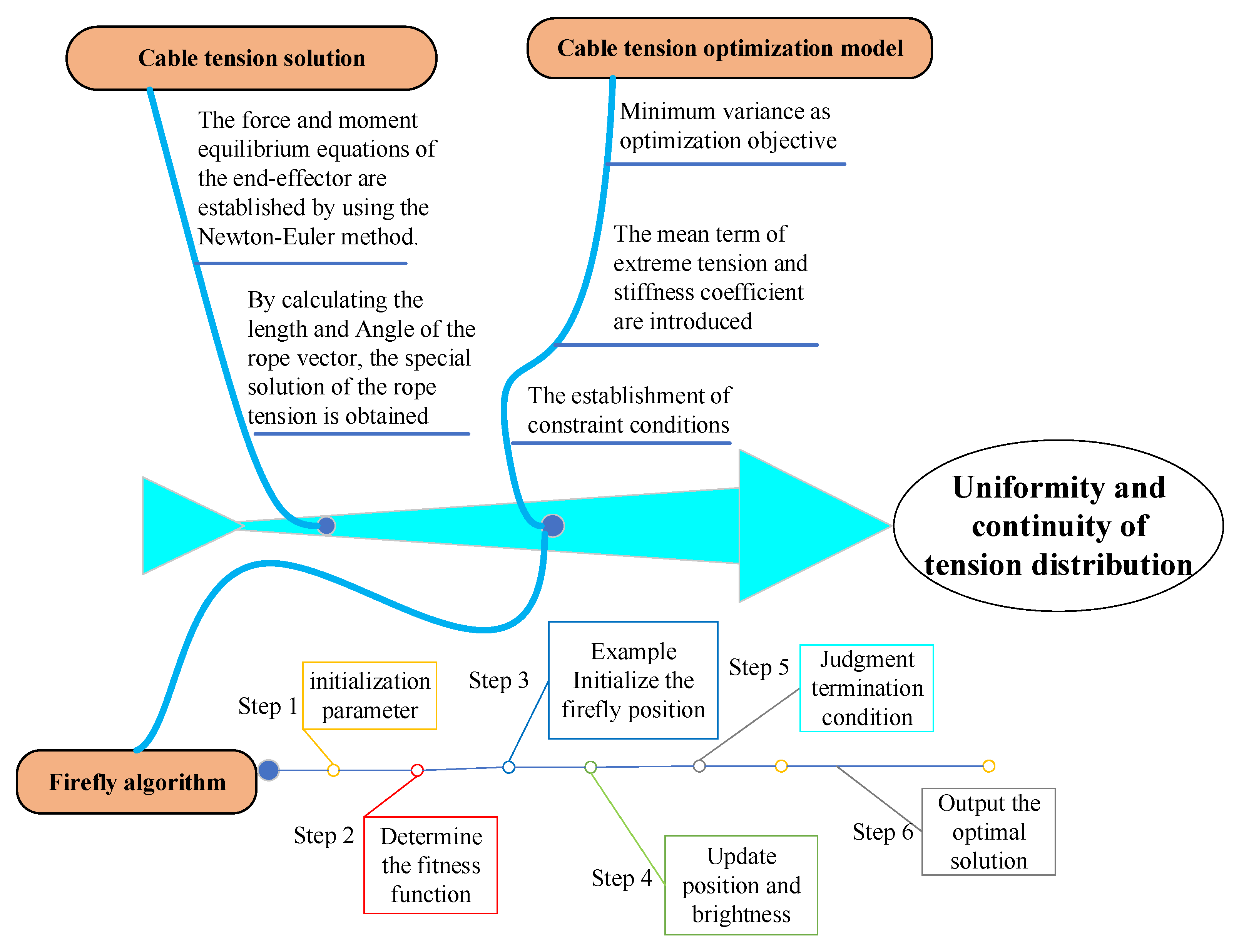
4.1. Cable Tension Optimization Process

The process of solving and optimizing the cable tension of a cable-driven parallel robot includes two key steps. As shown in Figure 5, firstly, the force and moment equilibrium equations of the end-effector are established using the Newton–Euler method. By calculating the length and angle of the cable vector, a special solution for the cable tension is obtained. Then, to improve the minimum variance of tension distribution as the optimization goal, the tension average term related to the stiffness coefficient is introduced to ensure the uniformity and continuity of tension distribution. Specifically, the optimization goal is to further balance the tension distribution by introducing a stiffness coefficient so that the tension variance of each cable is minimized. In order to ensure the reliability of the system, the force and moment balance equation of the end effector and the protection against virtual traction and overload are used as constraints to keep the cable tension within the predetermined range. Based on these optimization objectives and constraints, an optimization model is constructed that takes into account the minimization of tension variance, the minimization of stiffness influence, and the minimization of force torque balance constraints. According to the firefly algorithm, the optimal solution is obtained by initializing variables, setting algorithm parameters, determining fitness function, initializing firefly position, updating position and brightness, and determining termination conditions.

4.2. Cable Tension Optimization Model

In order to operate steadily for the robot, the huge tension difference between any two cables needs to be avoided. Therefore, it is of great importance for cable tension distribution to make the tension difference between any two cables as small as possible. So, the minimum variance is selected as the optimization objective of the tension distribution. When the end-effector of the cable-drive parallel robot operates normally, the ith cable tension must be within a range, i.e.,

$$T_{i,\min }\le T_i\le T_{i,\max }, i=1,2,\dots ,8$$

(14)

Setting ${\mathit{T}}_{\min }={[T_{1,\min },T_{2,\min },T_{3,\min },T_{4,\min },T_{5,\min },T_{6,\min },T_{7,\min },T_{8,\min }]}^{{\rm T}}\in R^{m\times 1}$, it is the minimum preload required for each cable to ensure it can invariably be under the tension state when the end-effector is moving. And letting ${\mathit{T}}_{\max }=[T_{1,\max },T_{2,\max },T_{3,\max },T_{4,\max },T_{5,\max },T_{6,\max }$, $T_{7,\max },T_{8,\max }{]}^{{\rm T}}\in R^{m\times 1}$, it is the maximum allowable tension determined by the cable’s material strength that guarantees that the cable is not damaged and broken.

As a result, the tension distribution problem is transformed into a constraint optimization problem, and the optimization model is as follows:

$$\begin{array}{l}\mathit{Objective}\begin{array}{c}\begin{array}{cc}\begin{array}{cc}\begin{array}{cc}\begin{array}{cc}\begin{array}{cc}& \end{array}& \end{array}& \end{array}& \min \end{array}& \end{array}\end{array}F\left(x\right)\\ \mathit{Constraint}\begin{array}{cc}\begin{array}{cc}& \end{array}& \begin{array}{cc}\begin{array}{cc}\begin{array}{cc}& \end{array}& s.t.\end{array}& \end{array}\end{array}\left\{\begin{array}{l}m\dot{v}+G_e={\displaystyle \sum _{i=1}^8{T}_i+F_r}\\ I\dot{\omega }+\omega \times I\omega ={\displaystyle \sum _{i=1}^8{r}_i\times T_i+M_r}\\ T_{\min }(i)\le ‖T_i‖\le T_{\max }(i), i=1,2,\dots ,8\end{array}\right.\end{array}$$

(15)

$T_{\min }(i)$ is the ith element of $T_{\min }$. It is true for $T_{\max }(i)$. To improve the traditional minimum variance method, the tension extreme average term is introduced to change the tension around the average of the extreme tension and make the tension distribution more uniform and continuous. The objective function F(x) to be optimized can be expressed as follows:

$$F\left(x\right)=\min \left({\displaystyle \frac{1}{m}}\left[{\displaystyle \sum _{i=1}^m{\left(T_i-E\left(T\right)\right)}^2}\right]\right)$$

(16)

$$E\left(T\right)=\mathsf{\Gamma }\overline{T_i}+\overline{T}$$

(17)

In the Equation (17), $\mathsf{\Gamma }$ is the stiffness improvement coefficient, and the stiffness performance of the system can be adjusted by changing the coefficient. m is the number of cables. $\overline{T}$ is the average value of all tensions, i.e.,

$$\overline{T}=\left(T_1+T_2+T_3+T_4+T_5+T_6+T_7+T_8\right)/m$$

(18)

And $\overline{T_i}$ average value of ith cable’s tension, which can make the cable tension evenly distributed. $\overline{T_i}$ could be calculated by

$$\overline{T_i}=\left(T_{\min }+T_{\max }\right)/2$$

(19)

4.3. The Solution of Cable Tension

The end-effector’s force and torque are shown in Figure 6. Setting $r_i={[r_{i,x},r_{i,y},r_{i,z}]}^{{\rm T}},i=1,2,\dots ,8$, on the basis of the Newton–Euler method, the balance equation of the end-effector’s force and torque is as follows:

$$\left\{\begin{array}{l}{\displaystyle \sum _{i=1}^8{T}_i{s}_{{\theta }_i}{c}_{{\varphi }_i}}+F_{r,x}=m{\dot{v}}_x\\ {\displaystyle \sum _{i=1}^8{T}_i{s}_{{\theta }_i}{s}_{{\varphi }_i}}+F_{r,y}=m{\dot{v}}_y\\ {\displaystyle \sum _{i=1}^8{T}_i{c}_{{\theta }_i}}+F_{r,z}=m{\dot{v}}_z\\ {\displaystyle \sum _{i=1}^8\left(r_{i,y}{T}_i{c}_{{\theta }_i}-r_{i,z}{T}_i{s}_{{\theta }_i}{s}_{{\varphi }_i}\right)}+M_{r,x}=I_{xx}{\dot{\omega }}_x+I_{xy}{\dot{\omega }}_y+I_{xz}{\dot{\omega }}_z+h_x\left({\omega }_x,{\omega }_y,{\omega }_z\right)\\ {\displaystyle \sum _{i=1}^8\left(-r_{i,x}{T}_i{c}_{{\theta }_i}-r_{i,z}{T}_i{s}_{{\theta }_i}{c}_{{\varphi }_i}\right)}+M_{r,y}=I_{xy}{\dot{\omega }}_x+I_{yy}{\dot{\omega }}_y+I_{yz}{\dot{\omega }}_z+h_y\left({\omega }_x,{\omega }_y,{\omega }_z\right)\\ {\displaystyle \sum _{i=1}^8\left(r_{i,x}{T}_i{s}_{{\theta }_i}{c}_{{\theta }_i}-r_{i,y}{T}_i{s}_{{\theta }_i}{s}_{{\varphi }_i}\right)}+M_{r,z}=I_{xz}{\dot{\omega }}_x+I_{yz}{\dot{\omega }}_y+I_{zz}{\dot{\omega }}_z+h_z\left({\omega }_x,{\omega }_y,{\omega }_z\right)\end{array}\right.$$

(20)

where

$$s_{{\theta }_i}=\sin ({\theta }_i),c_{{\theta }_i}=\cos ({\theta }_i),s_{{\varphi }_i}=\sin ({\varphi }_i),c_{{\varphi }_i}=\cos ({\varphi }_i)$$

(21)

$$\left\{\begin{array}{l}{h}_x\left({\omega }_x,{\omega }_y,{\omega }_z\right)={\omega }_z(I_{xy}{\omega }_x+I_{yy}{\omega }_y+I_{yz}{\omega }_z)+{\omega }_y(I_{xz}{\omega }_x+I_{yz}{\omega }_y+I_{zz}{\omega }_z)\\ h_y\left({\omega }_x,{\omega }_y,{\omega }_z\right)={\omega }_z(I_{xx}{\omega }_x+I_{xy}{\omega }_y+I_{xz}{\omega }_z)-{\omega }_x( I_{xz}{\omega }_x+I_{yz}{\omega }_y+I_{zz}{\omega }_z)\\ h_z\left({\omega }_x,{\omega }_y,{\omega }_z\right)={\omega }_y(I_{xx}{\omega }_x+I_{xy}{\omega }_y+I_{xz}{\omega }_z)+{\omega }_x(I_{xy}{\omega }_x+I_{yy}{\omega }_y+I_{yz}{\omega }_z)\end{array}\right.$$

(22)

In Equation (20), ${\theta }_i(i=1,2,\dots ,8)$ is the angle between the tension $T_i$ and $z_I$ axis. ${\varphi }_i$ is the angle between $x_I$ axis and the projection of $T_i$ on the plane $x_I{o}_I{y}_I$. ${\dot{v}}_x$, ${\dot{v}}_y$, and ${\dot{v}}_z$ are the linear acceleration of the end-effector along $x_I$, $y_I$ and $z_I$ axis, respectively. ${\dot{\omega }}_x$, ${\dot{\omega }}_y$ and ${\dot{\omega }}_z$ are the angular acceleration of the end-effector along $x_I$, $y_I$ and $z_I$ axis, respectively.${\omega }_x$, ${\omega }_y$ and ${\omega }_z$ are the angular velocity of the end-effector, respectively.

The symbols $F_{r,x}$, $F_{r,y}$, and $F_{r,z}$ represent the external forces applied on the end effector along the $x_I$, $y_I$, and $z_I$ axis, respectively. The external torques around $x_I$, $y_I$, and $z_I$ axis denote $M_{r,x}$, $M_{r,y}$ and $M_{r,z}$. $h_x$, $h_y$, and $h_z$ are functions about ${\omega }_x$, ${\omega }_y$, and ${\omega }_z$, and they can be obtained by Equation (22). Assuming the inertia matrix of the end-effector is $I$, it can be yielded as follows:

$$I=\left[\begin{array}{ccc}{I}_{xx}& I_{xy}& I_{xz}\\ I_{yx}& I_{yy}& I_{yz}\\ I_{zx}& I_{zy}& I_{zz}\end{array}\right]$$

(23)

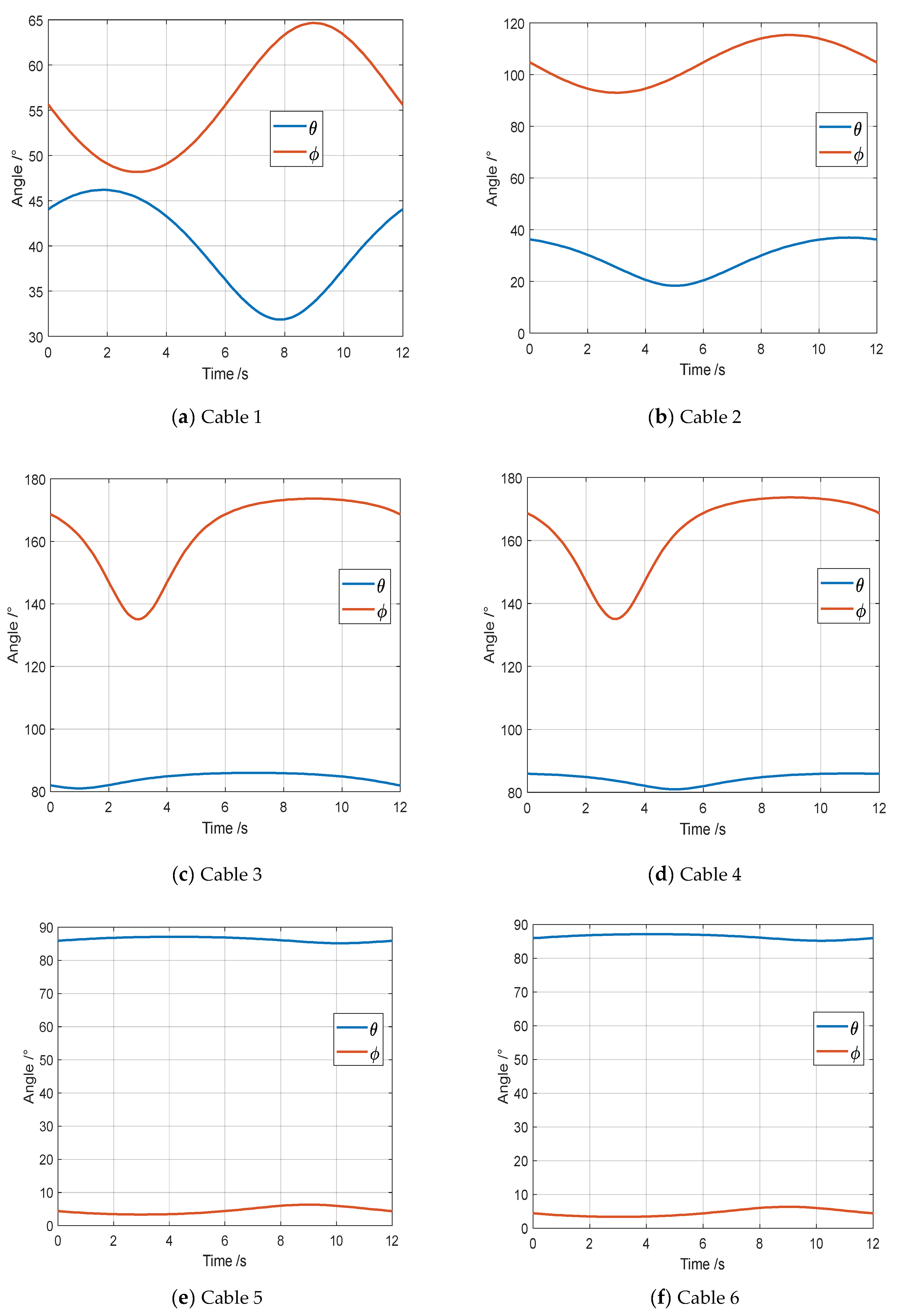
4.3.1. Calculation for Angle θ_i

According to previous content, the value of θ_i is determined by the apex of the end-effector (P_i) and the vertex of the frame (B_i), as shown in Figure 6. Setting the position coordinates of P_i and B_i are (P_i,x, P_i,y, P_i,z) and (B_i,x, B_i,y, B_i,z), respectively. Based on the Euclidean formula, the Euclidean distance between P_i and B_i is calculated as follows:

$$‖D_i‖=\sqrt{{(B_{i,x}-P_{i,x})}^2+{(B_{i,y}-P_{i,y})}^2+{(B_{i,z}-P_{i,z})}^2}$$

(24)

The θ_i represents the intersection angle between the position vector D_i and the positive direction of the $z_I$ axis. As a result, the cosine of θ_i is the projection of D_i along the z-axis. It can be obtained as follows:

$$\begin{array}{l}\cos ({\theta }_i)={\displaystyle \frac{D_i\cdot n_z}{‖D_i‖‖n_z‖}}={\displaystyle \frac{{\left[\begin{array}{ccc}{B}_{i,x}-P_{i,x}& B_{i,y}-P_{i,y}& B_{i,z}-P_{i,z}\end{array}\right]}^{{\rm T}}\cdot {\left[\begin{array}{ccc}0& 0& 1\end{array}\right]}^{\mathrm{T}}}{\sqrt{{(B_{i,x}-P_{i,x})}^2+{(B_{i,y}-P_{i,y})}^2+{(B_{i,z}-P_{i,z})}^2}}}\\ ={\displaystyle \frac{B_{i,z}-P_{i,z}}{\sqrt{{(B_{i,x}-P_{i,x})}^2+{(B_{i,y}-P_{i,y})}^2+{(B_{i,z}-P_{i,z})}^2}}}\end{array}$$

(25)

where n_z is the unit vector along the z-axis.

Based on the Equation (25), the angle θ_i can be calculated by

$${\theta }_i=\arccos \left({\displaystyle \frac{B_{i,z}-P_{i,z}}{\sqrt{{(B_{i,x}-P_{i,x})}^2+{(B_{i,y}-P_{i,y})}^2+{(B_{i,z}-P_{i,z})}^2}}}\right)$$

(26)

4.3.2. The Determination of the Angle ϕ_i

As shown in Figure 6, angle ϕ_i represents the intersection angle between the projection of D_i on the plane $x_I{o}_I{y}_I$ and the positive direction of $x_I$ axis. The projection of D_i on the plane $x_I{o}_I{y}_I$ is obtained as follows:

$${\stackrel{⌢}{D}}_i={\left[\begin{array}{ccc}{D}_i\cdot n_x& D_i\cdot n_y& 0\end{array}\right]}^{{\rm T}}={\left[\begin{array}{ccc}{B}_{i,x}-P_{i,x}& B_{i,y}-P_{i,y}& 0\end{array}\right]}^{{\rm T}}$$

(27)

where n_x and n_y are unit vectors along the x-axis and y-axis, respectively.

So, the cosine of ϕ_i could be calculated as follows:

$$\cos ({\varphi }_i)={\displaystyle \frac{{\stackrel{⌢}{D}}_i\cdot n_x}{‖{\stackrel{⌢}{D}}_i‖‖n_x‖}}={\displaystyle \frac{{\left[\begin{array}{ccc}{B}_{i,x}-P_{i,x}& B_{i,y}-P_{i,y}& 0\end{array}\right]}^{{\rm T}}\cdot {\left[\begin{array}{ccc}1& 0& 0\end{array}\right]}^{\mathrm{T}}}{\sqrt{{(B_{i,x}-P_{i,x})}^2+{(B_{i,y}-P_{i,y})}^2}}}={\displaystyle \frac{B_{i,x}-P_{i,x}}{\sqrt{{(B_{i,x}-P_{i,x})}^2+{(B_{i,y}-P_{i,y})}^2}}}$$

(28)

On the basis of the Equation (25), the angle ϕ_i is obtained by

$${\varphi }_i=\arccos \left({\displaystyle \frac{B_{i,x}-P_{i,x}}{\sqrt{{(B_{i,x}-P_{i,x})}^2+{(B_{i,y}-P_{i,y})}^2}}}\right)$$

(29)

4.4. Optimization Algorithm Design

In the paper, the firefly algorithm is used to optimize the cable tension. The main steps are listed as follows: The specific process is shown in Figure 7.

(1)

Initialize parameters. First of all, the initial parameters are set, such as the robot structure parameters and time parameters. The robot parameters are the vertex coordinate $B_i=\left(\begin{array}{ccc}{x}_{Bi}& y_{Bi}& z_{Bi}\end{array}\right)$ and the end effector vertex $P_i=\left(\begin{array}{ccc}{x}_{Pi}& y_{Pi}& z_{Pi}\end{array}\right)$. And the maximum iteration parameter is $t_{\max }=1000$ in the time parameters.

(2)

Set the FA algorithm parameters. These are the population size $N=50$, the attraction parameter γ = 1.0, and the initial attraction ${\beta }_0=0.2$.

(3)

Randomly initialize the firefly position. The positions of individual fireflies are randomly initialized, and each firefly corresponds to a tension distribution solution. The initial brightness is calculated from the fitness function, assuming that the initial tension value is randomly distributed between the preset minimum tension $T_{\min }$ and the maximum tension $T_{\max }$.

$$T_i=T_{\min }+(T_{\max }-T_{\min })\cdot rand$$

(30)

(4)

Determine the fitness function. The fitness function is the objective function of the optimization problem. The objective of the optimization is to minimize the variance of the cable tension distribution and introduce the stiffness coefficient to make the tension distribution more uniform and continuous. The objective function is Equation (16).

(5)

The introduction of force and moment equation constraints. When calculating the fitness function, it is necessary to ensure that the cable tension satisfies the balance equation of force and moment. The force and moment balance equation of the cable robot is shown in Equation (32). In the fitness function calculation, a penalty term should be introduced to constrain these conditions:

$$F_{penaity}=\lambda (\parallel {\displaystyle \sum _{i=1}^8{T}_i+F_r}{\parallel }^2+\parallel {\displaystyle \sum _{i=1}^8{r}_i\times T_i+M_r}{\parallel }^2)$$

(31)

The final fitness function is:

$$F_{total}(x)=F(x)+F_{penaity}$$

(32)

(6)

Position update: update the position of fireflies according to step (4) and recalculate the brightness of fireflies according to Equation (14).

$$T_i^{new}=T_i+{\beta }_0{e}^{-\gamma r_{ij}^2}(T_j-T_i)+\alpha (rand-0.5)$$

(33)

where $r_{ij}$ is the distance between firefly $i$ and firefly $j$, $\alpha$ is the random parameter, and rand is the random number between them.

(7)

Judge the termination condition: check whether the error of the solution is less than the given precision or whether the number of iterations is greater than the maximum number of iterations. If the conditions are met, the optimal solution is output, and optimization is completed; otherwise, return to Step 5 to continue the iteration.

(8)

Output the globally optimal solution to tension and complete the optimization.

4.5. Factors Affecting Minimum Cable Tension

In order to determine the more important parameter of this minimum from the tension equation, the tension distribution of the cable robot needs to be analyzed from multiple angles. The key parameters include cable preload, material strength limit, cable length variation, stiffness coefficient, and so on. The following is a detailed analysis and description of these parameters.

4.5.1. Cable Preload

The pretension force of the cable is the key parameter to ensure that the cable always stays in a tensioned state. The choice of preload force directly affects the range of tension variation in the cable in different motion states. If the preload is too low, the cable may relax, causing the system to lose control. If the preload is too high, it will increase the burden on the cable and drive system and may even cause the cable to break.

4.5.2. Strength Limitation of Cable Material

The material strength limit of the cable is the maximum tension that the cable can withstand, and this parameter is determined by the material properties of the cable. Excessive tension will cause the cable to break, which will affect the safety and stability of the system.

4.5.3. Cable Length Changes

The variation in cable length is determined by the trajectory of the end effector. It is an important parameter affecting the tension distribution. During the movement of the end effector, the length of each cable will change, which will affect the tension distribution of the cable. The length variation in each cable is calculated according to the displacement of the end effector and the cable geometry.

4.5.4. Stiffness Coefficient

The stiffness coefficient is an important parameter used to measure the stiffness of a cable system. Improving the rigidity of the system is helpful to improve its stability and control accuracy.

The above parameters are the key factors that affect the tension distribution of the cable robot. By setting and optimizing these parameters reasonably, the minimum value of the tension equation can be reduced effectively. In the specific optimization process, the firefly algorithm and other optimization methods are used to find the optimal parameter combination through iterative calculation so that the tension distribution is more uniform and continuous.

5. Simulation Study

To verify the proposed method is valid for the optimization of tension, a cable-driven parallel robot, shown in Figure 8, is taken as an example for the simulation study. In the simulation, MATLAB software (https://www.mathworks.com/products/matlab.html) is used to simulate the trajectory of the end effector and optimize the tension of the cable.

The parameters of the robot are listed in

Table 3. Parameters of the robot.

Item	Value	Unit
The size of the end-effector	100 × 100 × 100	mm
The number of driven cables	8	/
Degree of freedom for the end-effector	6	/

. Parameters of the robot.

The envelope size of the robot is 1000 mm × 1000 mm × 1000 mm. The size of the end-effector is 100 mm × 100 mm × 100 mm. The robot is driven by eight cables made of the same material. However, there are only 6 DOFs for the end-effector, i.e., three translation motions and three rotation motions in 3D space.

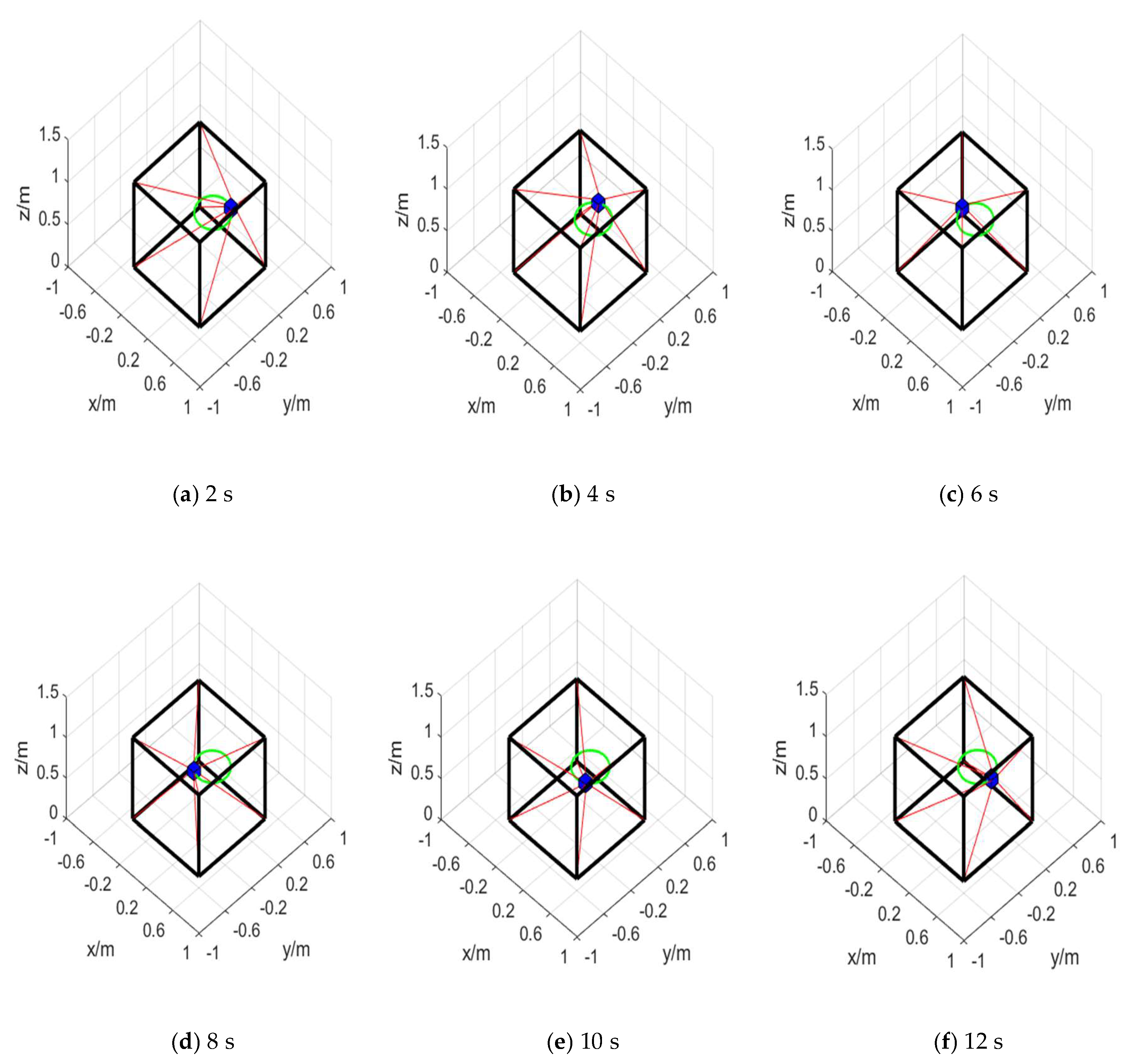
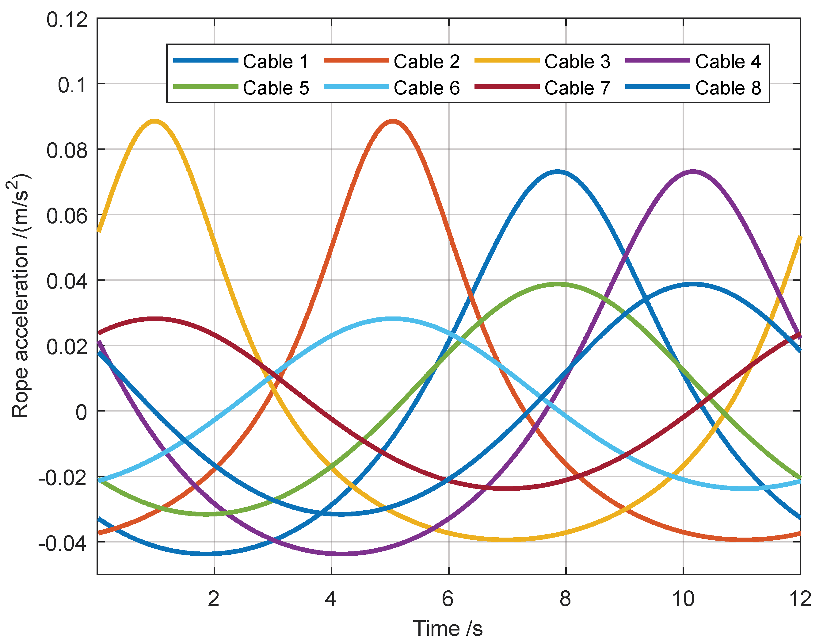
5.1. The Simulation for the End-Effector’s Motion

Here, a spatial arc trajectory, as shown in Figure 9, is designed for the end-effector of the cable-driven parallel robot to trace.

The arc is determined by O_c, R_c, and n_c three parameters. O_cis the center of the arc. R_c is the vector from the center to the initial point of the arc. n_c is the normal vector of the plane where the arc is. As a consequence, for any point on the arc, its position vector is obtained as follows:

$$P_c=O_c+e^{\eta \cdot n_c^{\times }}\cdot R_0$$

(34)

$$e^{\eta \cdot n_c^{\times }}=I+\sin \left(\eta \right)\cdot n_c^{\times }+\left(1-\cos \left(\eta \right)\right)\cdot n_c^{\times }\cdot n_c^{\times }$$

(35)

where η is the corresponding central angle of $P_c$.

In the simulation, the parameters of the spatial arc are set as follows:

$$\left\{\begin{array}{l}{O}_c={\left[\begin{array}{ccc}0.0\mathrm{m}& 0.2\mathrm{m}& 0.5\mathrm{m}\end{array}\right]}^{{\rm T}}\\ R_0={\left[\begin{array}{ccc}0.0\mathrm{m}& 0.0\mathrm{m}& 0.2\mathrm{m}\end{array}\right]}^{{\rm T}}\\ n_c={\left[\begin{array}{ccc}0& 0& 1\end{array}\right]}^{{\rm T}},\eta \in [0^{\circ }, {360}^{\circ }]\end{array}\right.$$

(36)

Combining Equation (34) and Equation (36), the values of $P_c$ in x, y, and z are obtained as follows:

$$\left\{\begin{array}{l}{P}_{cx}=0.2\cos (\omega t)+0\\ P_{cy}=0.2\sin (\omega t)+0.2\\ P_{cz}=0.5\end{array}\right.$$

(37)

Here, the simulation step size is set as 0.1 s, and the simulation time is 12 s. According to the simulation results, some states of the end-effector at different times during the simulation are shown in Figure 10. As illustrated in Figure 11, it represents the included angle ${\theta }_i$ and ${\varphi }_i$ for each cable.

Figure 10 shows the movement trajectories of the end-effector at different time points. These six subgraphs show changes in the position of the end effector from 0 s to 12 s. Through the observation of these trajectories, it can be seen that the end effector maintains a smooth and continuous trajectory during the whole motion, which indicates the effectiveness of the optimization algorithm.

Figure 11 shows the changing process of the angle ${\theta }_i$ and angle ${\varphi }_i$ under the circular trajectory movement. Each subgraph (a–h) corresponds to the change in angle between cables 1 and 8. As shown in

Table 4. The range of angles ${\theta }_i$ and ${\varphi }_i$.

Cable 1–8	${\mathit{\theta }}_{\mathit{i}}$ Angle Range	${\mathit{\varphi }}_{\mathit{i}}$ Angle Range
Cable 1	${45}^{\circ }<{\theta }_1<{30}^{\circ }$	${45}^{\circ }<{\varphi }_1<{65}^{\circ }$
Cable 2	${15}^{\circ }<{\theta }_2<{40}^{\circ }$	${90}^{\circ }<{\varphi }_2<{120}^{\circ }$
Cable 3	${80}^{\circ }<{\theta }_3<{90}^{\circ }$	${130}^{\circ }<{\varphi }_3<{170}^{\circ }$
Cable 4	${80}^{\circ }<{\theta }_4<{90}^{\circ }$	${135}^{\circ }<{\varphi }_4<{170}^{\circ }$
Cable 5	$0^{\circ }<{\theta }_5<{10}^{\circ }$	${80}^{\circ }<{\varphi }_5<{90}^{\circ }$
Cable 6	$0^{\circ }<{\theta }_6<{10}^{\circ }$	${80}^{\circ }<{\varphi }_6<{90}^{\circ }$
Cable 7	${15}^{\circ }<{\theta }_7<{40}^{\circ }$	${90}^{\circ }<{\varphi }_7<{110}^{\circ }$
Cable 8	${30}^{\circ }<{\theta }_8<{50}^{\circ }$	${45}^{\circ }<{\varphi }_8<{65}^{\circ }$

, it is the variation range of the sum of the eight ropes under the circular trajectory.

In Figure 11a,b,g,h, that is, in the time range of 0 s to 12 s for cable 1, cable 2, cable 7, and cable 8, the variation range of angle ${\theta }_i$ and angle ${\varphi }_i$ is large, indicating that the cable needs to make a large attitude adjustment to adapt to the trajectory motion during the entire motion process. Among them, the extreme value of angle ${\theta }_i$ of cable 1 appears near 3 s and 9 s, the extreme value of angle ${\varphi }_i$ appears near 2 s and 8 s, the extreme value of angle ${\theta }_i$ of cable 2 appears near 3 s and 9 s, the extreme value of angle ${\varphi }_i$ appears near 2 s and 8 s, the extreme value of angle ${\theta }_i$ of cable 7 appears near 3 s and 9 s, and the extreme value of angle ${\varphi }_i$ appears near 1 s and 7 s. The extreme value of the angle ${\theta }_i$ of cable 8 appears near 3 s and 9 s, and the extreme value of the angle ${\varphi }_i$ appears near 2 s and 8 s. In Figure 11e,f, the change range of angle ${\theta }_i$ and angle ${\varphi }_i$ of cable 5 and cable 6 from 0 s to 12 s is relatively gentle. That is, the cable maintains a relatively stable attitude adjustment. In Figure 11c,d, the angle ${\theta }_i$ of cable 3 and cable 4 shows a minimum at 3 s, while the angle ${\varphi }_i$ changes more gently.

Based on the inverse kinematics of the cable-driven parallel robot, when the position and attitude of the end-effector are known, the variation in the cables’ length can also be obtained. It is shown in Figure 12. The variation range of cables’ length is from −0.6 m to 0.6 m. The negative number represents the pulling of the cable. Otherwise, the release of cables is denoted by a positive number. Moreover, the linear velocity and linear acceleration of each cable are calculated and illustrated in Figure 13 and Figure 14. The velocity of each cable is changed from −0.1 m/s to 0.1 m/s, and the variation range of the cables’ acceleration is between −0.05 m/s² and 0.1 m/s². It can be concluded that the variation in length, velocity, and acceleration is continuous and smooth, and there is no step change. So, all cables will not tremble or quiver, which is very important for the cable functioning of the cable-driven parallel robot and also demonstrates the effectiveness of the inverse solution algorithm.

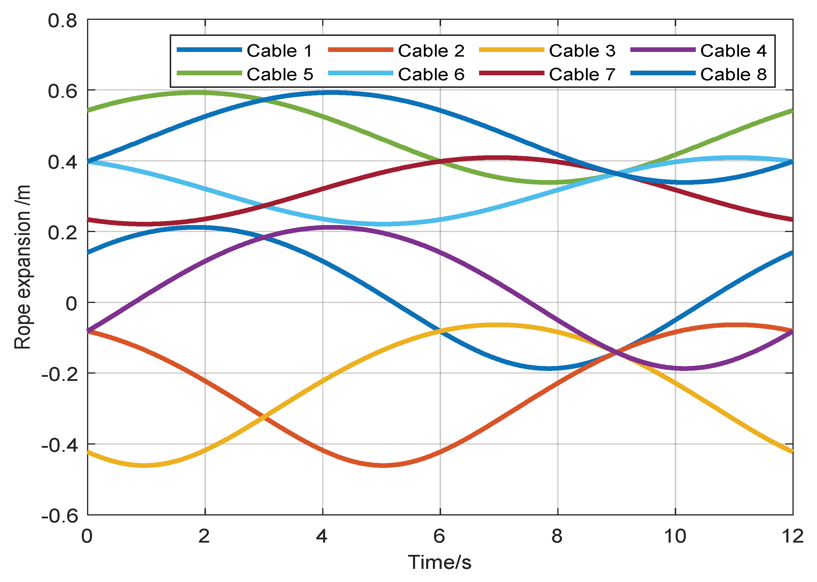
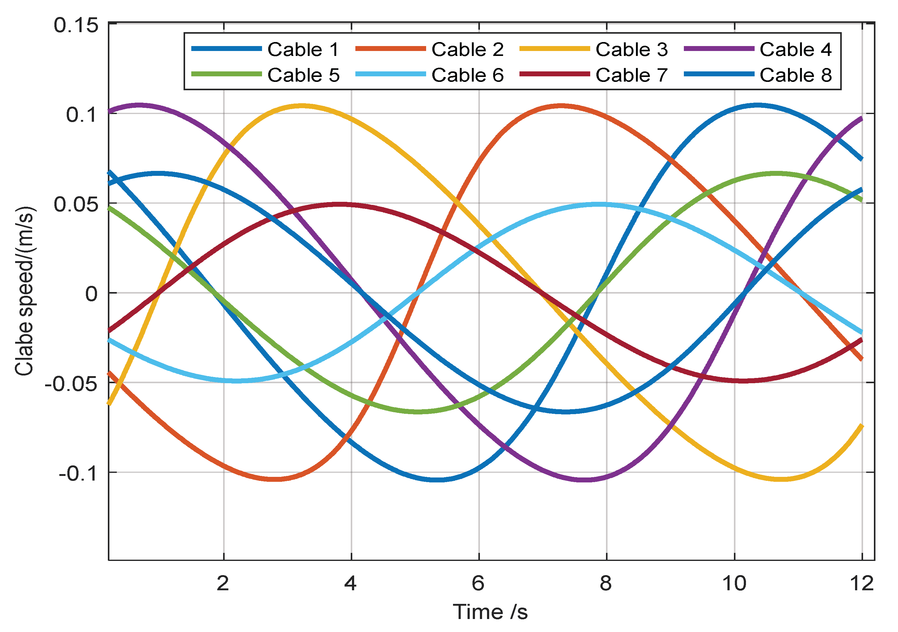
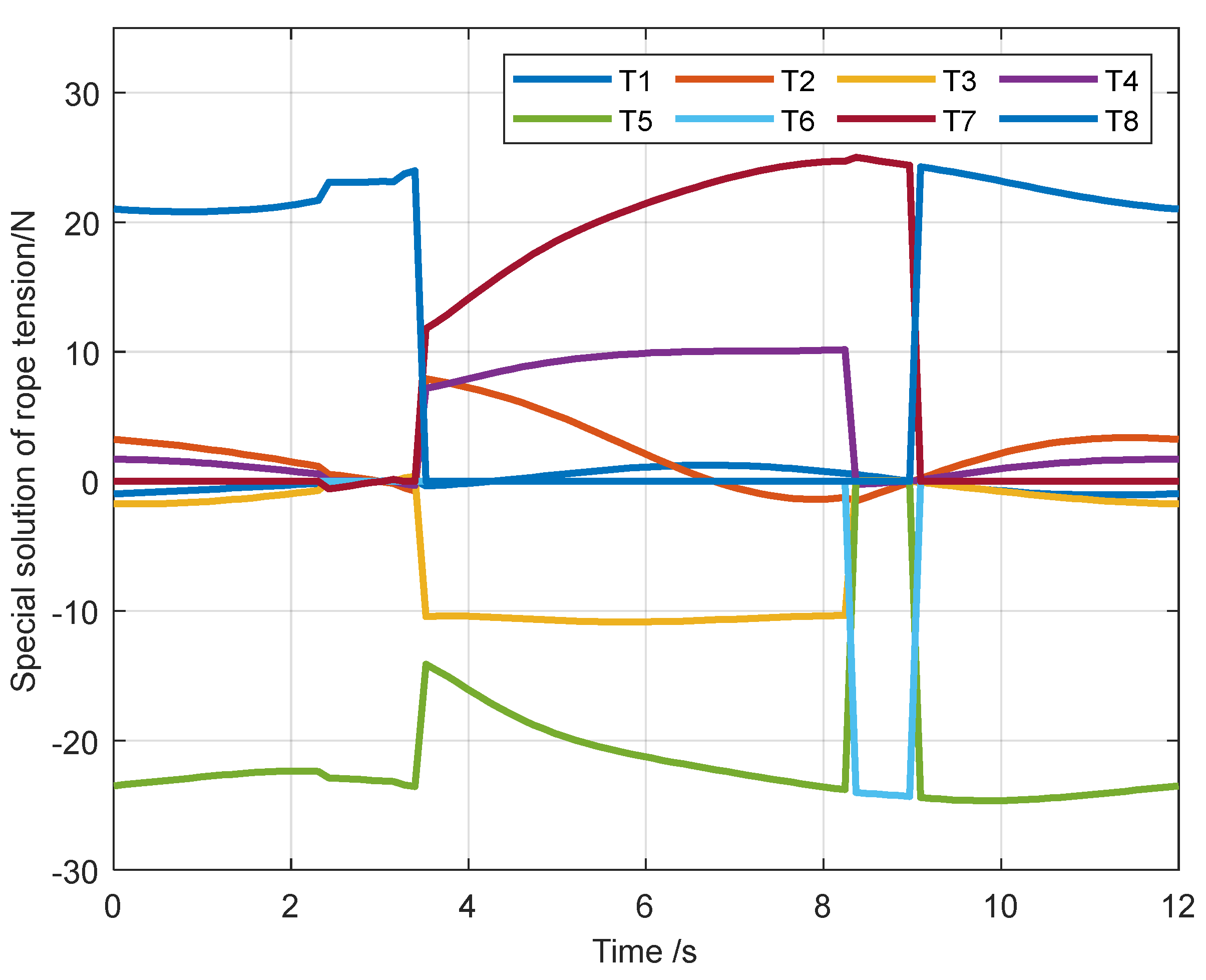
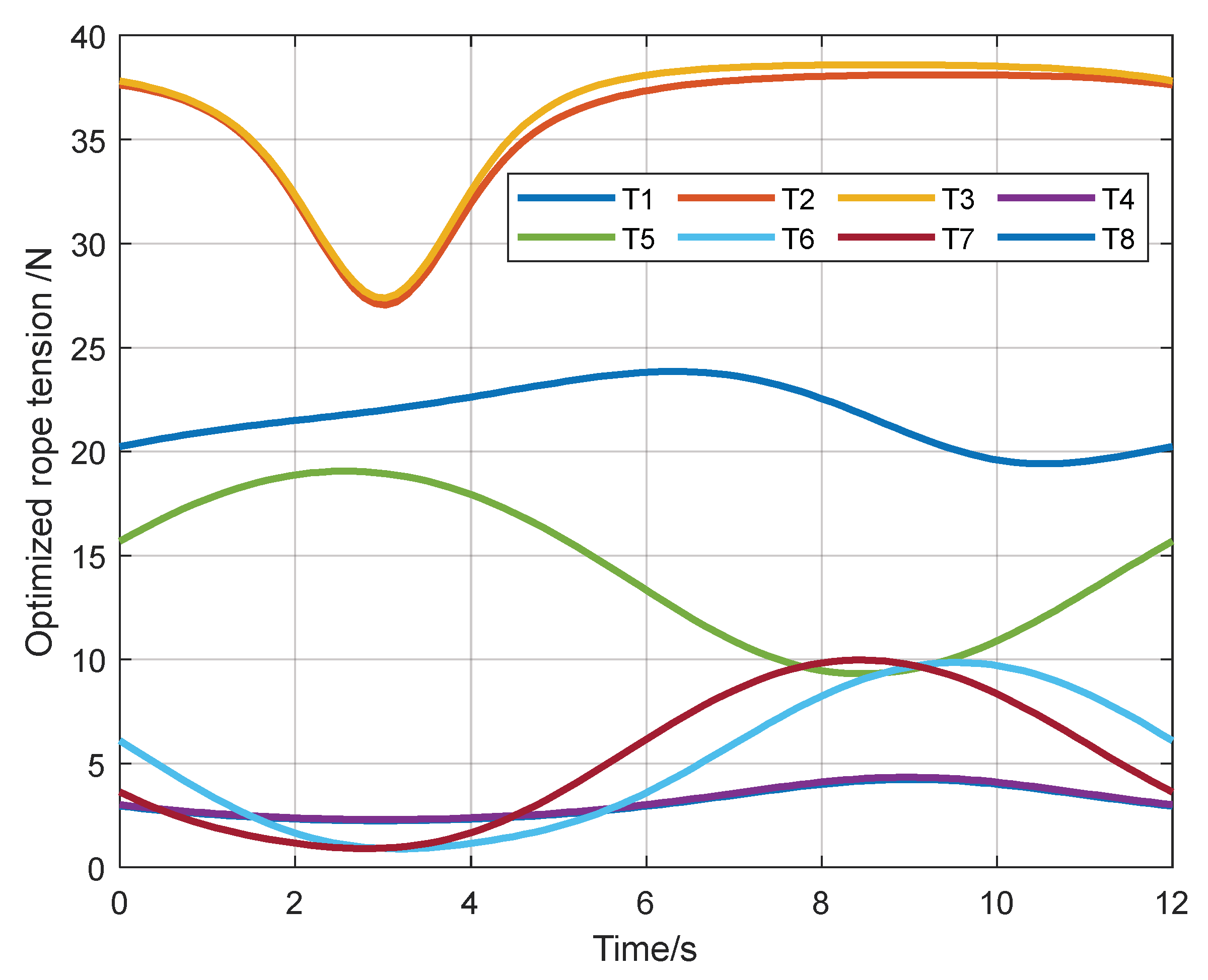
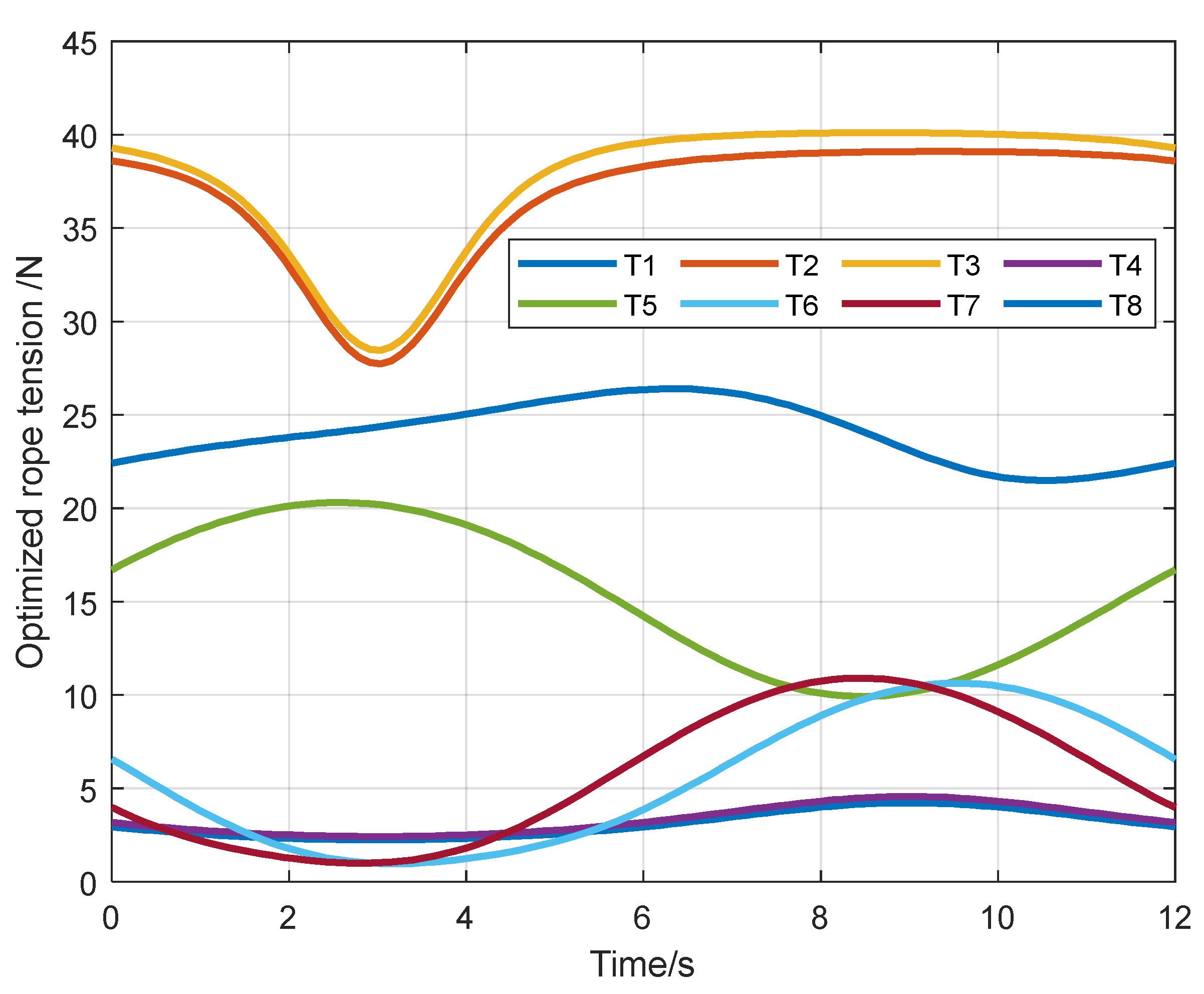
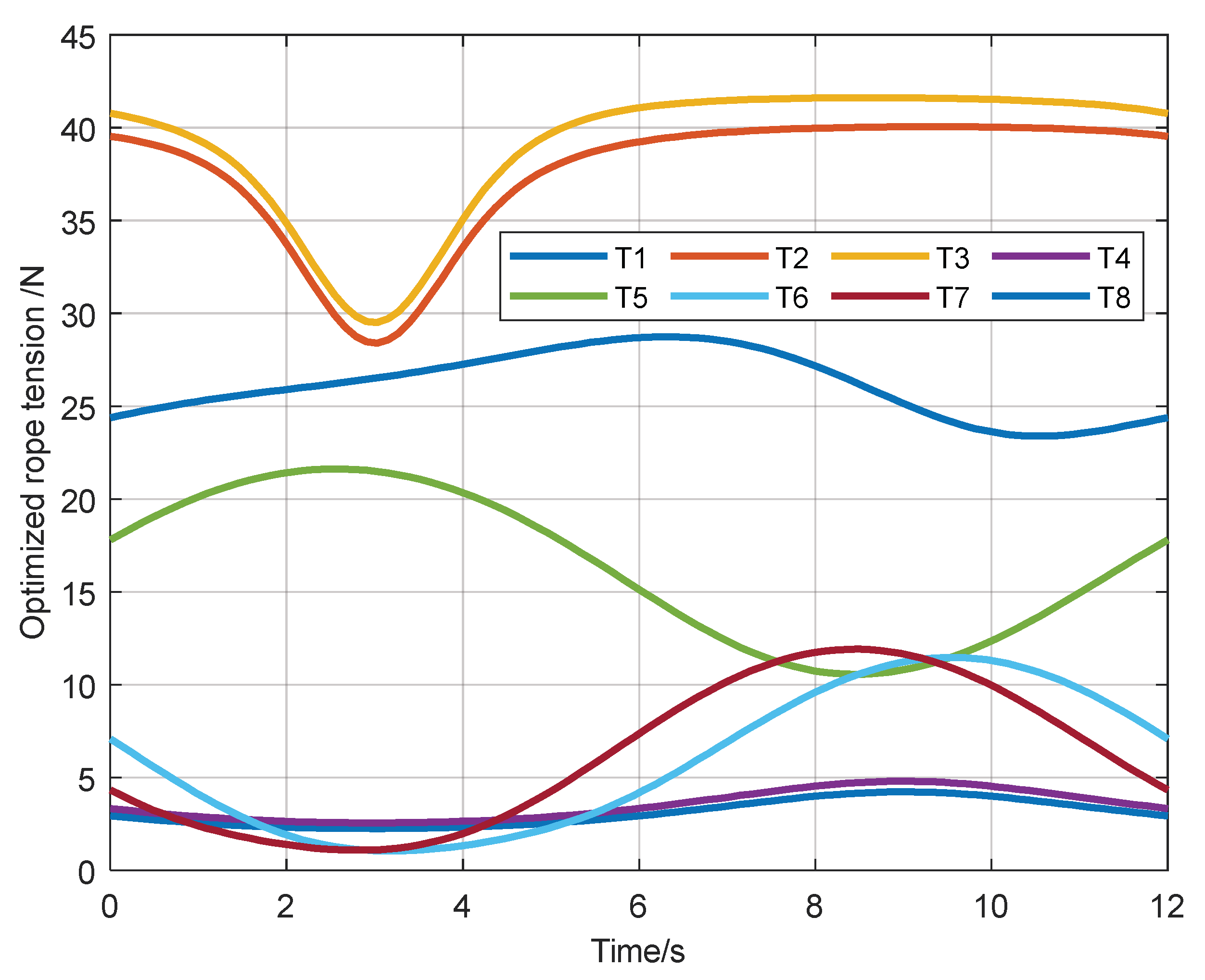
5.2. The Simulation for the Tension Optimization

As discussed above, when the pose, velocity, and acceleration are determined, there are finite sets of tension distributions that can satisfy the dynamics equation of the robot.

As can be obtained from Figure 15, the change curve of the cable tension special solution term is not smooth, and its value is negative, which is inconsistent with the actual experience, so the cable tension should be optimized through the general solution term.

Figure 16, Figure 17 and Figure 18 show the optimized cable tension, which can be obtained from the figure. After optimization, the tension curves of the four cables change continuously and steadily. At the initial moment, the tension of 1, 2, 3, and 5 of the cable is greater than the tension of 4, 6, 7, and 8. At the same time, it can be found that the higher the stiffness improvement coefficient is, the larger the average cable tension is, and the system stiffness is improved, but at the same time, the maximum cable tension is larger, and the maximum will cause the fatigue fracture of the cable. Considering the rigidity and cable strength of the system, it is suggested that the stiffness improvement coefficient should be 0.2 in the future test or simulation of the cable-driven parallel device.

6. Conclusions

The cable tension distribution of cable-driven parallel robots is one of the research focuses because it has a direct impact on the movement characteristics. To make the cable tension distribution more continuous and even, an optimization method based on the firefly algorithm is proposed for the tension distribution of cables. The structural design of the parallel robot is introduced in detail. The dynamic equation of the cable-driven parallel robot is derived from the Newton–Euler method. Then, an optimization algorithm for cable tension based on minimum variance optimization is presented to solve the problems of the insufficient stiffness of the optimized system and the discontinuity and non-uniqueness of cable tension. Finally, a simulation model is built using MATLAB software to verify the proposed method. The following conclusions can be obtained:

(1)

The cable tension optimization method introduced by minimum variance is adopted so that the optimized cable tension is evenly distributed near the average value of the preset extreme tension, and the optimization range of the tension is determined by the extreme tension value.

(2)

Taking the improved minimum variance of the correlation force as the optimization objective and using the improved minimum variance method to optimize the cable tension, the change in cable tension by the proposed method is smoother than that of the traditional method. In addition to this, all cable tension curves are continuous. Nevertheless, they are discontinuous for traditional methods.

It should be pointed out that this paper mainly considers optimization when cables are not. In the future, we will strive to do further research on cable tension distribution, taking into account the plastic deformation of cables.

References

1. Zarebidoki, M.; Dhupia, J.S.; Xu, W. A review of cable-driven parallel robots: Typical configurations, analysis techniques, and control methods. IEEE Robot. Autom. Mag. 2022, 29, 89–106. [Google Scholar] [CrossRef]
2. Mishra, U.A.; Caro, S. Forward kinematics for suspended under-actuated cable-driven parallel robots with elastic cables: A neural network approach. J. Mech. Robot. 2022, 14, 041008. [Google Scholar] [CrossRef]
3. Liu, Q.; Ye, L. Design and Research for Industrial Robot Using Goods Sorting in Warehouse. In Proceedings of the 2022 WRC Symposium on Advanced Robotics and Automation (WRC SARA), Beijing, China, 20 August 2022; IEEE: Piscataway, NJ, USA, 2022. [Google Scholar]
4. Zaccaria, F.; Idá, E.; Briot, S.; Carricato, M. Workspace computation of planar continuum parallel robots. IEEE Robot. Autom. Lett. 2022, 7, 2700–2707. [Google Scholar] [CrossRef]
5. Hou, S.H.; Tang, X.Q.; Cao, L.; Cui, Z.-W.; Sun, H.-H.; Yan, Y.-W. Research on end-force output of 8-cable driven parallel manipulator. Int. J. Autom. Comput. 2020, 17, 378–389. [Google Scholar] [CrossRef]
6. Rodriguez-Barroso, A.; Saltaren, R. Tension planner for cable-driven suspended robots with unbounded upper cable tension and two degrees of redundancy. Mech. Mach. Theory 2020, 144, 103675. [Google Scholar] [CrossRef]
7. McDonald, E.; Arsenault, M.; Beites, S. Design of a Suspended Cable-Driven Parallel Robot for The Semi-automation of Construction Tasks. In Proceedings of the Canadian Committee for the Theory of Machines and Mechanisms, Québec City, QC, Canada, 19–20 June 2023. [Google Scholar]
8. Laribi, M.A.; Carbone, G.; Zeghloul, S. On the optimal design of cable driven parallel robot with a prescribed workspace for upper limb rehabilitation tasks. J. Bionic Eng. 2019, 16, 503–513. [Google Scholar] [CrossRef]
9. Zhao, Y.; Liang, C.; Gu, Z.; Zheng, Y.; Wu, Q. A new design scheme for intelligent upper limb rehabilitation training robot. Int. J. Environ. Res. Public Health 2020, 17, 2948. [Google Scholar] [CrossRef] [PubMed]
10. Liu, J.; Zhang, A.; Li, E.; Guo, R. A review on the environment perception and control technologies for the hyperredundant manipulators in limited space. J. Sens. 2022, 2022, 7659012. [Google Scholar] [CrossRef]
11. Qian, S.; Bao, K.; Zi, B.; Wang, N. Kinematic calibration of a cable-driven parallel robot for 3D printing. Sensors 2018, 18, 2898. [Google Scholar] [CrossRef] [PubMed]
12. Jung, J. Workspace and stiffness analysis of 3D printing cable-driven parallel robot with a retractable beam-type end-effector. Robotics 2020, 9, 65. [Google Scholar] [CrossRef]
13. Zhang, B.; Shang, W.; Cong, S.; Li, Z. Dual-loop dynamic control of cable-driven parallel robots without online tension distribution. IEEE Trans. Syst. Man Cybern. Syst. 2022, 52, 6555–6568. [Google Scholar] [CrossRef]
14. Wang, Y.; Wang, K.; Chai, Y.; Mo, Z. Research on mechanical optimization methods of cable-driven lower limb rehabilitation robot. Robotica 2022, 40, 154–169. [Google Scholar] [CrossRef]
15. Song, D.; Zhang, L.; Xue, F. Configuration optimization and a tension distribution algorithm for cable-driven parallel robots. IEEE Access 2018, 6, 33928–33940. [Google Scholar] [CrossRef]
16. Picard, E.; Caro, S.; Plestan, F.; Claveau, F. Stiffness oriented tension distribution algorithm for cable-driven parallel robots. In Advances in Robot Kinematics 2020; Springer International Publishing: Cham, Switzerland, 2021. [Google Scholar]
17. Ameri, A.; Molaei, A.; Khosravi, M.A. Nonlinear observer-based tension distribution for cable-driven parallel robots. In Proceedings of the 5th International Conference on Cable-Driven Parallel Robots, Virtual, 7–9 July 2021; Springer International Publishing: Cham, Switzerland, 2021. [Google Scholar]
18. Dao, C.H.K.; Tuong, P.T.; Vu, N.D.; Nguyen, M.N. On Research of Cable Tension Distribution Algorithm for Four Cables-Three DOF Planar Cable-Driven Parallel Robot. J. Tech. Educ. Sci. 2023, 18, 8–17. [Google Scholar] [CrossRef]
19. Chen, Y.; Li, J.; Wang, S.; Han, G.; Sun, Y.; Luo, W. Dynamic Modeling and Robust Adaptive Sliding Mode Controller for Marine Cable-Driven Parallel Derusting Robot. Appl. Sci. 2022, 12, 6137. [Google Scholar] [CrossRef]
20. Kieu, V.N.D.; Huang, S.-C. Dynamic and wrench-feasible workspace analysis of a cable-driven parallel robot considering a nonlinear cable tension model. Appl. Sci. 2021, 12, 244. [Google Scholar] [CrossRef]
21. Cao, S.; Luo, Z.; Quan, C. Real-Time Tension Distribution Design for Cable-Driven Parallel Robot. Appl. Sci. 2022, 13, 10. [Google Scholar] [CrossRef]
22. Pott, A.; Bruckmann, T.; Mikelsons, L. Closed-form force distribution for parallel wire robots. In Computational Kinematics, Proceedings of the 5th International Workshop on Computational Kinematics, Forsthausweg, Germany, 6–8 May 2009; Springer: Berlin/Heidelberg, Germany, 2009. [Google Scholar]
23. Pott, A. An improved force distribution algorithm for over-constrained cable-driven parallel robots. In Computational Kinematics: Proceedings of the 6th International Workshop on Computational Kinematics (CK2013), Barcelona, Spain, 20–22 May 2013; Springer: Dordrecht, The Netherlands, 2014. [Google Scholar]
24. Gouttefarde, M.; Lamaury, J.; Reichert, C.; Bruckmann, T. A versatile tension distribution algorithm for n-DOF parallel robots driven by n + 2 cables. IEEE Trans. Robot. 2015, 31, 1444–1457. [Google Scholar] [CrossRef]
25. Lim, W.B.; Yeo, S.H.; Yang, G. Optimization of tension distribution for cable-driven manipulators using tension-level index. IEEE/ASME Trans. Mechatron. 2013, 19, 676–683. [Google Scholar] [CrossRef]
26. Parque, V.; Miyashita, T. Optimal Design of Cable-Driven Parallel Robots by Particle Schemes. In Proceedings of the 29th International Conference on Neural Information Processing, Virtual, 22–26 November 2022; Springer Nature: Singapore, 2022. [Google Scholar]
27. Choe, W. A Design of Parallel Wire Driven Robots for Ultrahigh Speed Motion Based on Stiffiness Analysis. In Proceedings of the Japan-USA Symposium on Flexible Automation, Boston, MA, USA, 7–10 July 1996. [Google Scholar]
Figure 1. The overall structure of the cable-driven parallel robot.
Applsci 14 06478 g001
Figure 2. Machine design schematic.
Applsci 14 06478 g002
Figure 3. Schematic diagram of the cable guide path.
Applsci 14 06478 g003
Figure 4. Dynamic analysis diagram of a cable-driven parallel robot.
Applsci 14 06478 g004
Figure 5. Global optimization flow chart.
Applsci 14 06478 g005
Figure 6. Analysis of the end-effector’s force and torque.
Applsci 14 06478 g006
Figure 7. Flow diagram of the algorithm.
Applsci 14 06478 g007
Figure 8. The simulation model of the cabledriven parallel robot.
Applsci 14 06478 g008
Figure 9. Simulation trajectory of the end-effector.
Applsci 14 06478 g009
Figure 10. Simulated motion trajectory of the end-effector. (Red represents cable; Green represents the simulation trajectory of the end-effector; Blue represents the end effector; Black represents the robot frame).
Applsci 14 06478 g010
Figure 11. The change process of angle θ i and angle ϕ i under circular trajectory motion.
Applsci 14 06478 g011aApplsci 14 06478 g011b
Figure 12. Curve of cable expansion over time.
Applsci 14 06478 g012
Figure 13. Cable velocity curves over time.
Applsci 14 06478 g013
Figure 14. Curve of the cable acceleration over time.
Applsci 14 06478 g014
Figure 15. Cable tension before optimization.
Applsci 14 06478 g015
Figure 16. The stiffness improvement coefficient is 0.1.
Applsci 14 06478 g016
Figure 17. The stiffness improvement coefficient is 0.2.
Applsci 14 06478 g017
Figure 18. The stiffness improvement coefficient is 0.3.
Applsci 14 06478 g018