Featured Application
Image generation of steel microstructures, enhancing materials research, quality control, and education by providing efficient and accurate visual representations without extensive reliance on traditional microscopy.
Abstract
Characterizing the microstructures of steel subjected to heat treatments is crucial in the metallurgical industry for understanding and controlling their mechanical properties. In this study, we present a novel approach for generating images of steel microstructures that mimic those obtained with optical microscopy, using the deep learning technique of generative adversarial networks (GAN). The experiments were conducted using different hyperparameter configurations, evaluating the effect of these variations on the quality and fidelity of the generated images. The obtained results show that the images generated by artificial intelligence achieved a resolution of 512 × 512 pixels and closely resemble real microstructures observed through conventional microscopy techniques. A precise visual representation of the main microconstituents, such as pearlite and ferrite in annealed steels, was achieved. However, the performance of GANs in generating images of quenched steels with martensitic microstructures was less satisfactory, with the synthetic images not fully replicating the complex, needle-like features characteristic of martensite. This approach offers a promising tool for generating steel microstructure images, facilitating the visualization and analysis of metallurgical samples with high fidelity and efficiency.
1. Introduction
Artificial intelligence (AI) techniques are being applied across various scientific fields, with significant exploration in materials science, particularly metallurgy. Deep learning, a subset of AI, offers innovative approaches for quantitatively studying material properties and observing microstructure images. Convolutional neural networks (CNNs) and other deep learning methods are employed for classification, segmentation, and feature extraction, facilitating expert analysis and advancing the understanding of process–structure–properties relationships [1,2,3,4,5,6]. These advancements in AI have led to improvements in steel quality control and microstructural analysis, highlighting the transformative potential of AI in metallurgy [7,8,9,10,11].
Another promising avenue is the generation of synthetic images using generative adversarial networks (GANs) [12], which offers a significant advantage for research [13,14,15,16,17,18,19]. One of the major challenges in materials science is the deficit of microstructure images due to the technical difficulty and cost of producing them. GANs can generate large amounts of synthetic data, providing a qualitative and quantitative leap in the study of microstructures, both in educational and research contexts. In recent years, GANs have been employed to generate realistic microstructural data efficiently [20,21,22,23,24].
Research in the field of steel and metallurgy, specifically involving GANs, has shown significant promise. Studies such as the work by Lee, J. et al. [25] emphasize the importance of predicting macro-scale material properties from microstructures. In this research, the investigators focused on creating and implementing various adversarial generative network models to produce highly authentic microstructural depictions of materials. Their dataset comprised light optical microscopy (LOM) and scanning electron microscopy (SEM) images of steel surfaces, showcasing microconstituents such as ferrite grains and mixed-phase constituents involving pearlites, retained austenite, and martensite. Additionally, the dataset included Li-battery cathode/anode microstructures. Using this diverse collection of images, they utilized three primary architectures: deep convolutional GAN (DCGAN), cycle-consistent GAN (Cycle GAN), and conditional GAN-based image-to-image conversion (Pix2Pix). Employing these frameworks, they fabricated virtual microscopic representations that closely mimicked the real microstructures present in their dataset.
The outcomes demonstrated that the AI-generated depictions were of superior quality, often indiscernible from authentic microscopic images to the unaided eye. The DCGAN yielded credible electron and optical microscopy representations of steel surfaces, accurately portraying the various microconstituents, while Cycle GAN enhanced this by producing higher-definition images and enabling style transference between optical and electron microscopy depictions. However, it should be noted that the training of the DCGAN did not specify or classify the microconstituents of steel, suggesting a non-supervised approach where all images were trained together without distinction. This lack of detailed labeling could limit the precision in generating specific microstructural features. Pix2Pix facilitated the creation of bespoke microstructures from hand-sketched designs, allowing for custom arrangements of ferrite, pearlite, austenite, and martensite.
Thakre, S. et al. [26] conducted a study to evaluate the capabilities of generative adversarial networks (GANs) in generating realistic microstructures of dual-phase (DP) steels, which are a heterogeneous mixture of soft ferrite and hard martensite phases. Using StyleGAN2, they generated microstructures from a limited dataset and assessed their similarity to real microstructures. Results indicated that while phase information was effectively captured, interface details were less accurate. Predictions of physical properties from GAN-generated microstructures aligned well with actual data, demonstrating that GANs can learn and reproduce relevant morphological features.
In another study, Narikawa, R. et al. [27] explored the application of GAN-based techniques to generate, translate, and enhance microstructural images of dual-phase (DP) steels, composed of soft ferrite and hard martensite phases. The study employed DCGAN to create realistic microstructures, CycleGAN for translating between optical and scanning electron microscopy images, and SRGAN to upscale low-resolution images. These methods produced high-quality virtual microstructures that were almost indistinguishable from real ones, effectively capturing phase information but showing less accuracy in interface details.
Sugiura, K. et al. [28] use a GAN approach for their study on steel image generation, employing SliceGAN to create 3D microstructure images from 2D images of ferrite-martensite dual-phase steels. This method significantly reduces the time required for 3D visualization. SliceGAN operates with a generator and discriminator working in tandem to produce precise 3D images. The study found that the martensite volume fractions in SliceGAN-generated images closely matched those in experimentally reconstructed images, highlighting SliceGAN’s effectiveness in 3D microstructural analysis and potential applications in materials science.
In a broader context of materials science, Jabbar et al. [29] also conducted experiments using GAN models to generate new material structures. Their datasets included information on atomic coordinates, lattice parameters, and various properties of crystal materials. The output of these GAN models primarily involved the creation of hypothetical crystal structures designed with specific desired properties such as band gaps, formation energy, and other physical characteristics. These structures were represented as data matrices, coordinate grids, or graphical models instead of conventional images, which is the focus of the present study.
The research demonstrated that GANs could efficiently generate microstructural data, facilitating advancements in data-driven materials design. Quantitative assessments, including phase fraction and morphology comparisons, showed that GAN-generated images accurately represented various microstructural features. The study suggests that combining GAN techniques with finite element method (FEM) analysis could further enhance the generation and utilization of materials data, supporting the design and optimization of microstructures based on desired properties. Despite achieving good results, there is room for improvement in the quality of optical images at resolutions higher than 256 × 256 pixels.
While several GAN architectures have been applied to microstructure image generation, each with varying success and limitations, our study focuses on the application of DCGANs for generating detailed steel microstructure images. Unlike CycleGAN and Pix2Pix, which excel in image-to-image translation tasks, DCGAN is specifically designed for generating realistic images from random noise vectors, making it well-suited for synthesizing steel microstructures. Additionally, the inclusion of various GAN architectures such as CycleGAN and SRGAN in comparative studies showcases the strengths and limitations of each approach, highlighting our unique contributions in optimizing DCGANs for producing outputs with higher resolution and achieving superior visual quality as assessed by domain experts.
This article is part of a series of previous publications by the authors specifically aimed at leveraging the advantages of artificial intelligence for interpreting carbon steel images. Initially, various machine learning algorithms were studied for classifying four types of steel using a public dataset of ultra-high-carbon steel microstructures (UHCSM), finding SVM to be the best classifier [30]. Subsequently, using our own dataset, a comparison was made between classic machine learning algorithms and deep learning for classifying images of steels subjected to annealing, quenching, and quenching with tempering, concluding that deep networks applying transfer learning with pre-trained models outperformed classical algorithms [31]. The topic of segmentation was also addressed using specific networks like DeepLabv3+, U-Net, and SegNet, with DeepLabv3+ with MobileNet as the feature extractor showing the best performance [32].
In this study, we explore the application of GANs to generate microstructures of annealed and quenched steels. Our focus is on optimizing hyperparameters through a trial-and-error process, constrained by GPU memory limitations. These constraints lead to realistic conditions in various environments where high-potential computing systems are unavailable. Our goal is to evaluate the impact of several hyperparameters, including the number of training epochs, learning rate, filter size, and batch size, on the quality of the generated images. The experiments presented here showcase the configurations that yielded the best results. We emphasize visual quality, as assessed by metallurgy experts, over purely quantitative metrics. It is crucial that the generated images convincingly replicate real microstructures to be considered successful. For our study, we utilized training images with a resolution of 512 × 512, which surpasses those found in existing literature.
2. Materials and Methods
2.1. Steel Samples and Dataset
To conduct the experiments, optical images of steel samples subjected to annealing and quenching heat treatments were used to obtain the microstructures of pearlite, ferrite, and martensite, independently. The steels used for obtaining micrographs were C25E and C45E for the annealing treatment and C45E, 37Cr4, and 34CrNiMo6 for the quenched steels. The detailed chemical composition of each is provided in Table 1.

Table 1.
Chemical composition (weight %) of low-carbon steel samples.
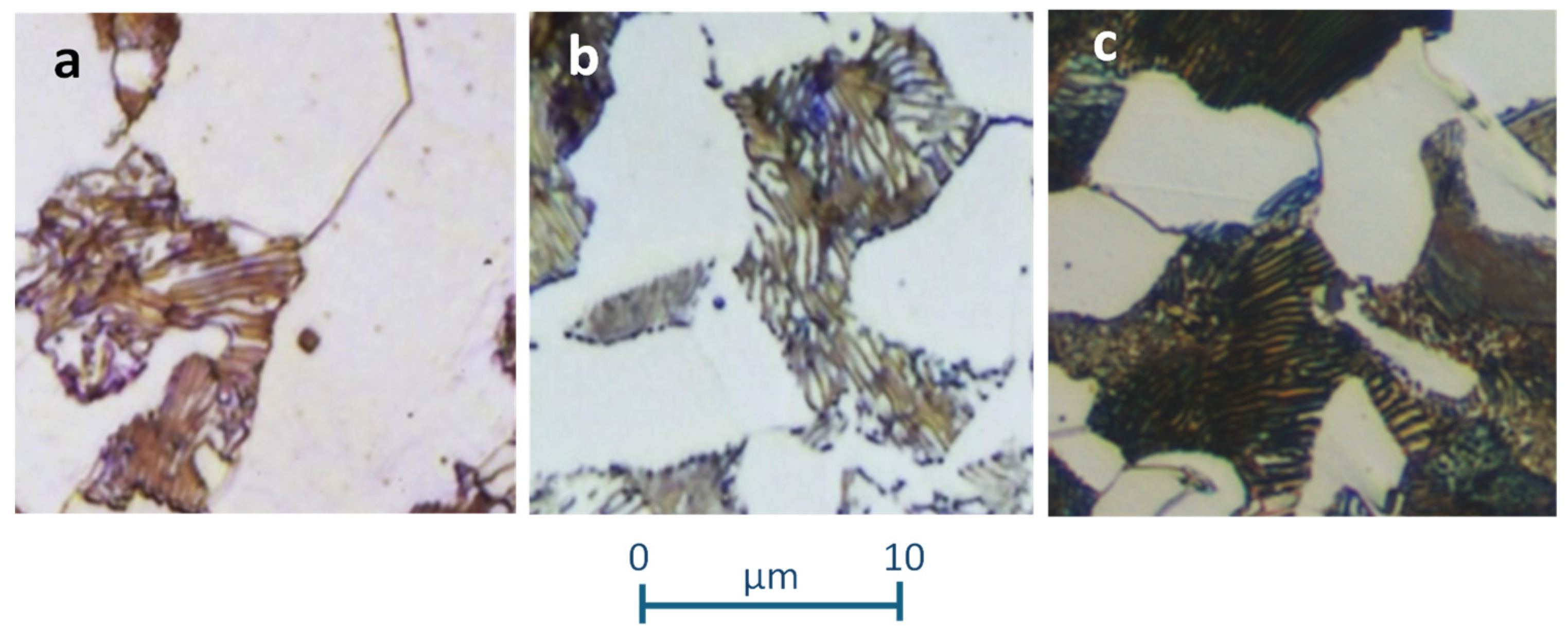
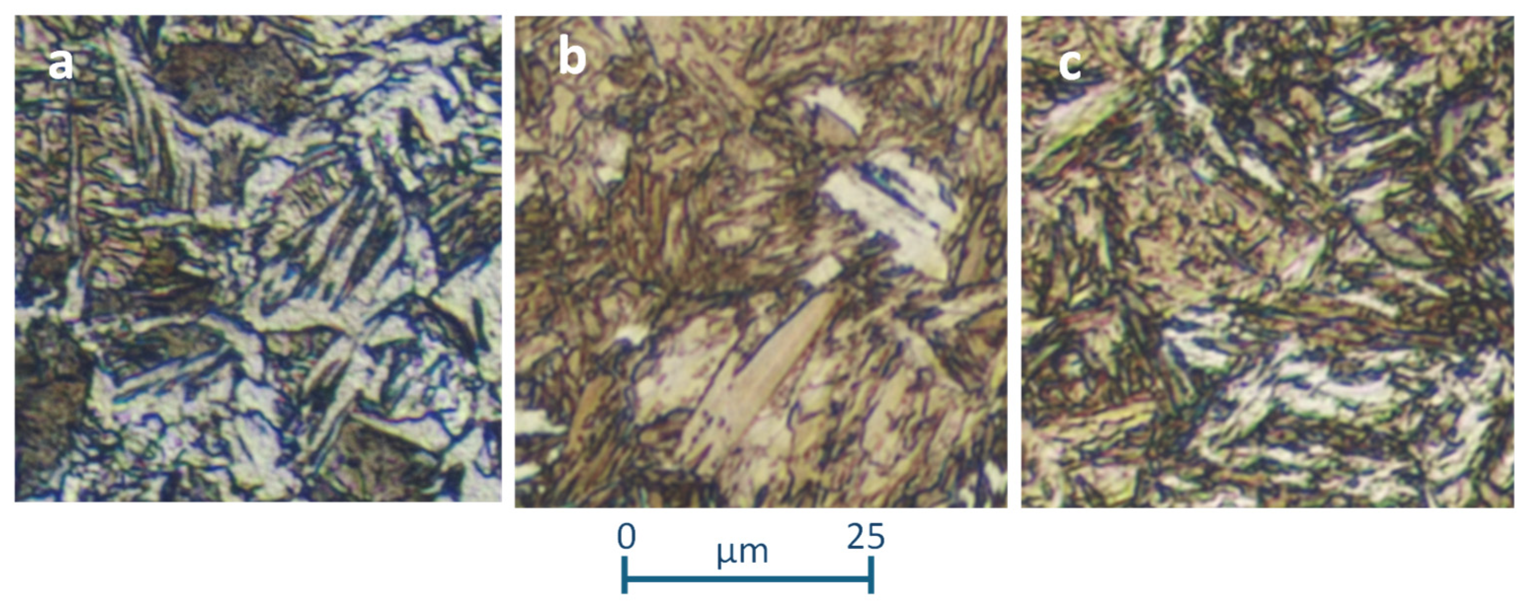
Following the heat treatments, the samples were prepared using the polishing procedure and chemical etching with Nital. The images were then obtained using an optical microscope at 400× and 1000× magnifications to distinguish different areas formed by steel microconstituents. The initial image dataset consists of 29 images for typical annealed samples and 40 for typical quenched samples, together a Widmanstätten structure, with a resolution of 2080 × 1542 pixels. Figure 1 and Figure 2 shows some samples where the areas of microconstituents generated in each heat treatment can be identified. In Figure 1, the lamellar area corresponds to pearlite and the white area to ferrite. The microstructures are very similar, although some heterogeneity has been included based on the carbon content of the steels (Table 1), as well as the cooling velocity during the treatment. Thus, Figure 1c presents a finer lamellar structure of the perlite due to the higher cooling velocity compared to Figure 1b.
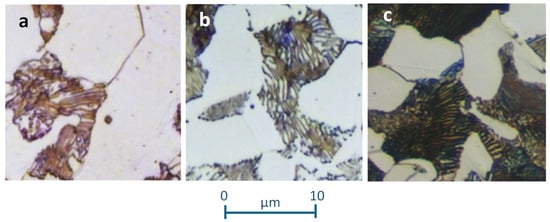
Figure 1.
Images of annealed steel samples showing microstructures with ferrite and pearlite (×1000). (a) C25E; (b) C45E steel; (c) C45E steel.
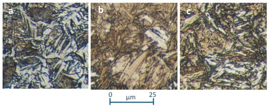
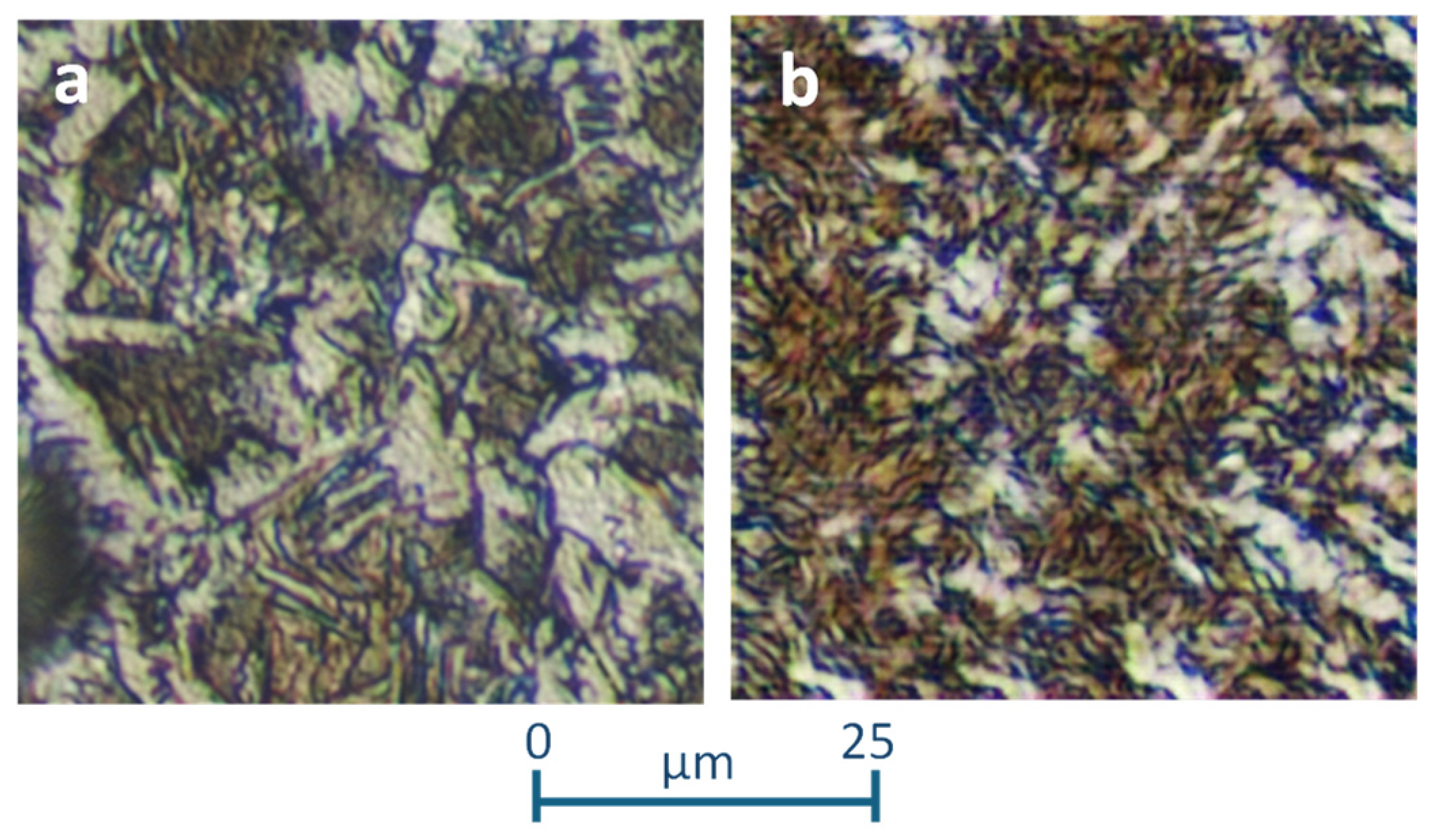
Figure 2.
Images (×400) of a Widmanstätten sample of a C25E steel (a), a complete martensite structure of a quenched 37Cr4 steel (b), and a martensite and lower bainite structure corresponding to a 34CrNiMo6 steel after an incomplete quenching treatment (c).
If the annealing treatment is carried out starting at a very high temperature, at which the austenite grains are large, the ferrite cannot nucleate at grain boundaries and the structure ferrite-perlite becomes atypical, receiving the name “Widmanstätten structure” (Figure 2a). Ferrite and perlite acquire acicular shapes in some way, which could create confusion for novice observers familiar with quenching structures. In any case, despite the acicular morphology of the microconstituents, the included heterogeneity remains relevant. Additionally, Figure 2c corresponds to a typical incomplete quenching treatment, where, besides the typical martensite appearing, some lower bainite can be observed. The appearance of the lower bainite is similar to the martensite but is more colored due to metallographic etching caused by existing inner Fe3C precipitates. The typical martensite coming from a complete quenching treatment can be observed in Figure 2b. Moreover, sometimes the three structures represented in Figure 2 can be obtained with high cooling velocities that sometimes are identified as quenching conditions; however, in reality, the results may be very different, as indicated above. The treatments referred to in Figure 2 have all been considered together in order to subject them to the methodology applied herein, as well as to evaluate the strength of the methodology under adverse conditions.
Once the image files were obtained, data augmentation [33,34] was implemented through cropping and rotation operations on the original images, increasing the number of images for training to 1392 for the annealed samples and 1440 for the quenched samples, with a resolution of 512 × 512 pixels.
2.2. Image Generative Models
In this study, we utilized DCGAN [35] for generating high-fidelity images of low-carbon steel microstructures. DCGANs consist of two neural networks: a generator and a discriminator. The generator creates synthetic images that mimic real optical microscopy images of low-carbon steel microstructures, while the discriminator evaluates their authenticity. Through iterative training, the generator improves its capability to produce realistic images. The DCGAN architecture was chosen for its effectiveness in producing high-quality and high-resolution images, closely resembling those obtained via traditional optical microscopy techniques.
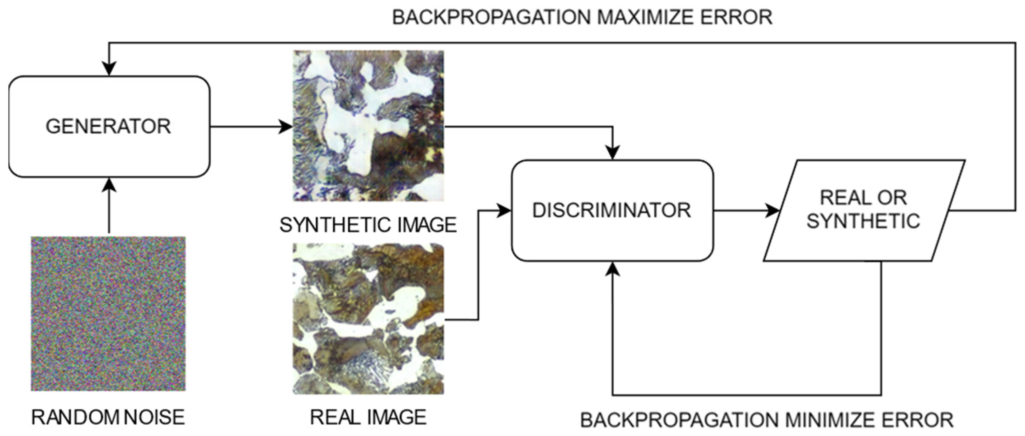
Figure 3 illustrates the schematic diagram of the DCGAN architecture used in this study. The generator network takes random noise as input and progressively transforms it into realistic images. In contrast, the discriminator network takes both real and generated steel images as input and functions as a classifier to distinguish between real and synthetic images. During the training process, both networks are updated iteratively. The discriminator is first trained on real images and synthetic images from the generator, with the goal of minimizing its classification error using a binary cross-entropy (BCE) loss function [36]. The generator is then trained to maximize the discriminator’s classification error by producing more realistic images, also using a BCE loss function but with the goal of making the discriminator classify synthetic images as real. This adversarial min-max optimization framework continues over many epochs, progressively enhancing the generator’s ability to produce highly realistic low carbon steel images that the discriminator cannot easily distinguish from real ones.
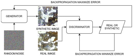
Figure 3.
Schematic diagram of the DCGAN architecture used for generating low-carbon steel microstructure images.
2.2.1. Generator Architecture
The generator network in our GAN is designed to transform a random noise vector Z of size 100 × 1 × 1 into a high-resolution image. The architecture consists of several transposed convolutional layers, each followed by batch normalization and ReLU activations, progressively upsampling the noise vector to the desired image dimensions. The layer structure and function can be described as follows:
Input Layer: The initial layer accepts the noise vector and applies a transposed convolution to increase spatial dimensions while reducing the number of feature maps.
Intermediate Layers: Subsequent layers continue this process, gradually refining the image. Each layer uses transposed convolutions to upsample the spatial dimensions, batch normalization to stabilize the learning process, and ReLU activations to introduce non-linearity, enabling the network to learn complex patterns.
Output Layer: The final transposed convolutional layer outputs a 512 × 512 image with 3 channels (RGB), scaled using a hyperbolic tangent (Tanh) activation function to the range [−1, 1].
The design parameters for the generator include a base number of 16 feature maps, following a sequence of 1024, 512, 256, 128, 64, 32, 16. This architecture ensures that the generator can produce detailed and high-quality images from a simple noise vector.
The detailed summary of the network, including the layer types, output shapes, and parameters is shown in Table 2. The generator network has a total of 12,825,312 parameters, all of which are trainable. The total computational complexity amounts to 55.18 giga multiply-adds (MACs).
Table 2.
Summary of the generator network architecture.
2.2.2. Discriminator Architecture
The discriminator distinguishes between real images from the dataset and synthetic images generated by the generator. The discriminator network takes an input image of size 512 × 512 with 3 channels (RGB) and processes it through a series of convolutional layers. The layer structure and function of the discriminator network is described below:
Input Layer: The initial convolutional layer reduces the image dimensions to 256 × 256 while increasing the number of feature maps to 16.
Intermediate Layers: Subsequent convolutional layers continue this process, halving the spatial dimensions and doubling the number of feature maps through layers 16, 32, 64, 128, 256, 512, and 1024. Batch normalization is applied to stabilize learning, and LeakyReLU activations introduce non-linearity.
Output Layer: The final layer outputs a single value using a Sigmoid activation function, representing the probability that the input image is real.
This architecture allows the discriminator to effectively learn and discern the nuanced differences between real and generated images, thereby providing feedback to the generator to improve its output.
A comprehensive overview of the network’s structure, including the layer types, output shapes, and parameters, is presented in Table 3. The network comprises 11,203,264 parameters, all of which are trainable, resulting in a total of 3.42 giga MACs.
Table 3.
Summary of the discriminator network architecture.
2.3. Training Loop
The training loop of the DCGAN involves initializing several essential components and iteratively updating the generator and discriminator networks. First, a binary cross-entropy loss function (BCELoss) is initialized to measure the discrepancy between real and synthetic outputs. A set of fixed latent vectors is used to monitor the generator’s progress, and smoothed labels for real and synthetic examples (real_label = 0.9, synthetic_label = 0.1) are employed to improve training stability. Adam optimizers are configured to update the parameters of both the generator (G) and discriminator (D) networks.
Extensive experiments were conducted to determine the optimal hyperparameters for the training process. The details of these hyperparameters are provided in Table 4. The training utilized one GPU, with the data loader using 2 workers.
Table 4.
Details of the experiments with relevant results. Common hyperparameters: Image Size = 512, Channels = 3, Latent Vector Size = 100, β1 = 0.5, β2 = 0.999, Filter Size = 4, Scale Parameter = 0.2, GPU = 1, Data Loader Workers = 2.
In each epoch and for each batch of data, the discriminator is first updated to minimize its classification error by correctly labeling real and generated samples. Then, the generator is updated to maximize the classification error of the discriminator by generating more realistic images that the discriminator classifies as real. During these updates, the losses are calculated, gradients are backpropagated, and network parameters are adjusted. Progress is monitored by periodically printing loss statistics and generating images from the fixed latent vectors to visualize the generator’s performance, as will be shown in the Results section. The impact of using different hyperparameters will be further examined in the Discussion section.
2.4. Experiments
Various experiments were conducted by modifying the hyperparameters of the model to evaluate their impact on the quality of the generated images. The hyperparameters modified include the number of training epochs, the learning rate (LR), the number of filters in each layer of the generator and discriminator, and the batch size. The experiments presented here produced the best results, with hyperparameters chosen through a trial-and-error process where GPU memory limitations played a crucial role in determining the best configuration.
In the Results section, only the experiments that produced qualitatively acceptable image generation in relation to the training images are included. Qualitative evaluation was performed by domain experts who compared the generated images with the real training images. The details of the three experiments that yielded relevant results are shown in Table 4.
2.5. Computational Resources
The experiments were performed on a computing system featuring an Intel(R) Core(TM) i7-5930K CPU @ 3.50 GHz, 64 GB of RAM, and an NVIDIA® GEFORCE RTX 3080 (10 GB). The software environment included the PyTorch framework, which was utilized for coding and producing image generation models. Specifically, PyTorch version 2.4.0 was used, along with CUDA version 12.1 to leverage GPU acceleration. The operating system was Ubuntu 20.04.6 LTS. All codes used in this research are available upon request to the authors.
3. Results
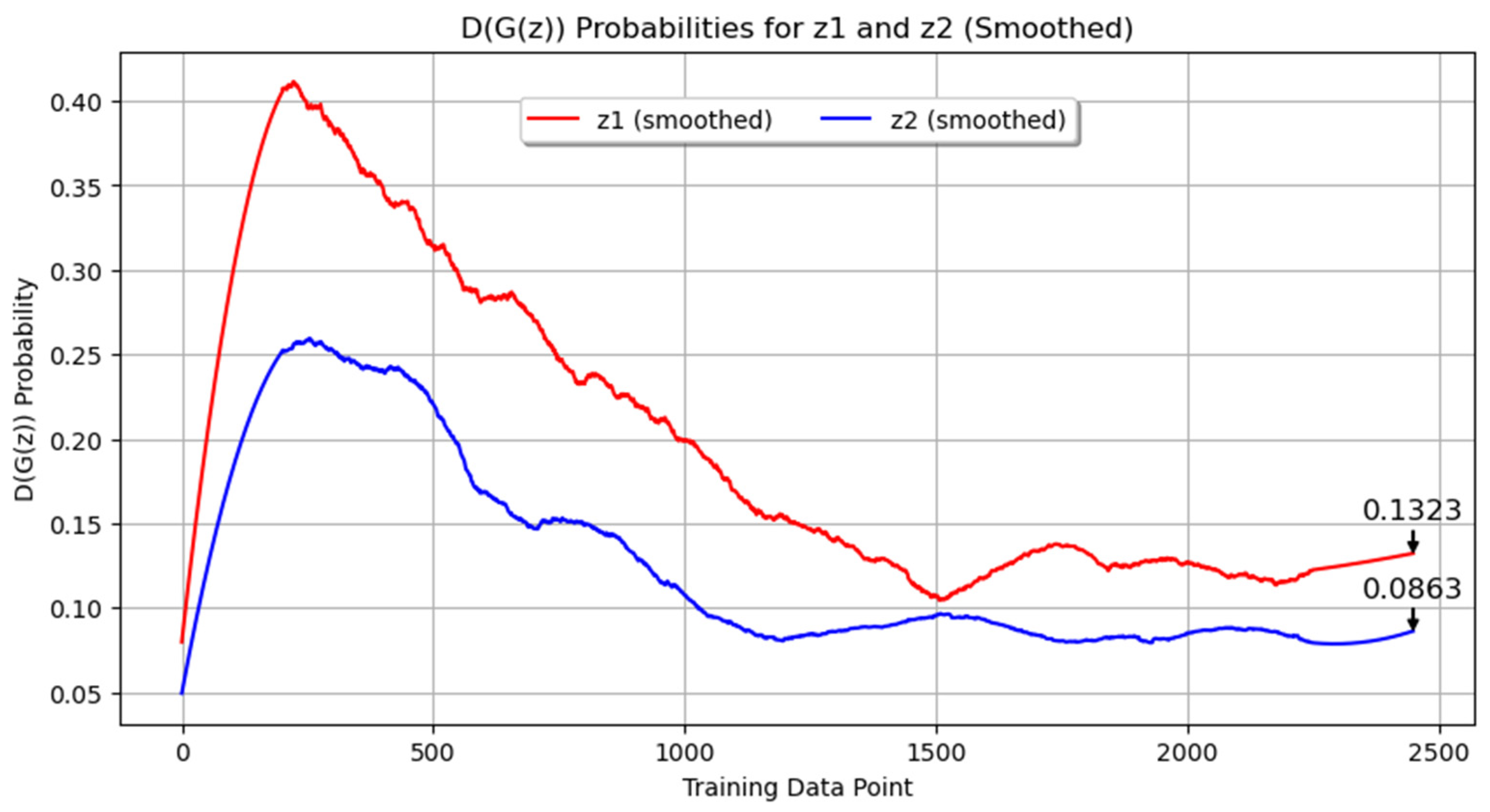
In this section, the outcomes from our experiments with the GAN architecture are detailed, and the best results achieved with the computational capabilities of the equipment are presented. The graphs of the generator and discriminator loss during training are included, and their significance is interpreted. Both the original training values and the smoothed values using the Savitzky–Golay filter [37] are represented for greater clarity. Additionally, the smoothed probability graphs D(G(z1)) and D(G(z2)) are included. Here, z1 refers to the latent vectors used to generate synthetic images, and z2 refers to the same latent vectors used for subsequent evaluations. D(G(z1)) is the discriminator’s probability that the images generated from z1 are real, evaluated before the generator is updated, while (G(z2)) is the probability that the images generated from z2 are real, evaluated after the generator update. These graphs provide qualitative insights into the discriminator’s ability to distinguish real images from generated ones throughout the training process. Following this, the impact of various hyperparameters on the quality of the generated images is discussed, with more detailed information provided in the Discussion section. The generated images are shown compared with the real images to illustrate the effectiveness of the training process.
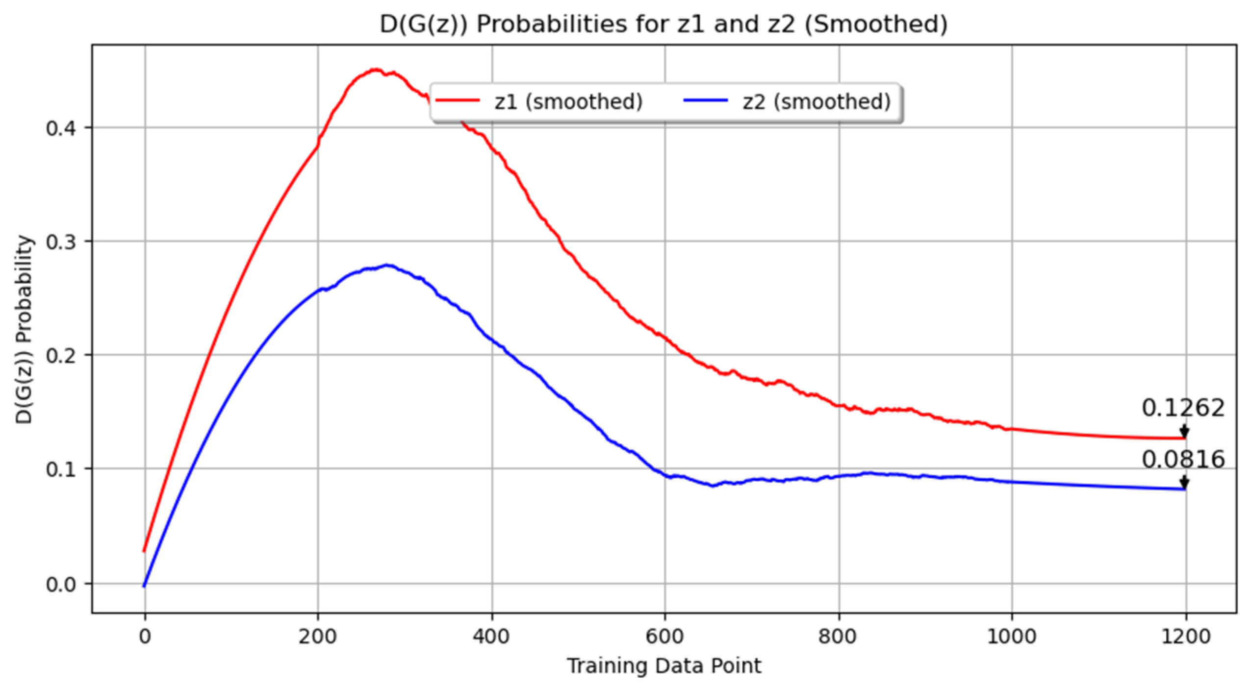
In our first experiment with annealed steel images, the GAN was trained for 350 epochs using a filter size of 16 and a batch size of 4. The training progress of the generator and discriminator losses are shown in Figure 4. Figure 4a presents the original data, while Figure 4b shows the smoothed data using the Savitzky–Golay filter. The final smoothed loss values were 2.3425 for the generator and 0.7181 for the discriminator. These results indicate that while the generator’s loss was consistently higher than the discriminator’s loss throughout the training process, both networks were actively learning. In Figure 5, the probability metrics D(G(z1)) and D(G(z2)) are depicted. D(G(z1)) is shown in red, while D(G(z2)) is shown in blue. Throughout the data log, D(G(z1)) remained consistently higher than D(G(z2)), with final values of 0.1323 and 0.0863, respectively. This suggests that the discriminator found it easier to identify images generated from z2 as synthetic compared to those from z1.
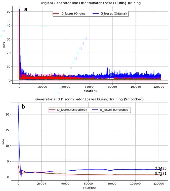
Figure 4.
Generator and discriminator loss during training for pearlite and ferrite image generation over 350 epochs with 16 filters and a batch size of 4. (a) Original; (b) Smoothed.
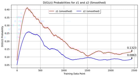
Figure 5.
Probability metrics for Experiment 1:D(G(z1)) and D(G(z2)).
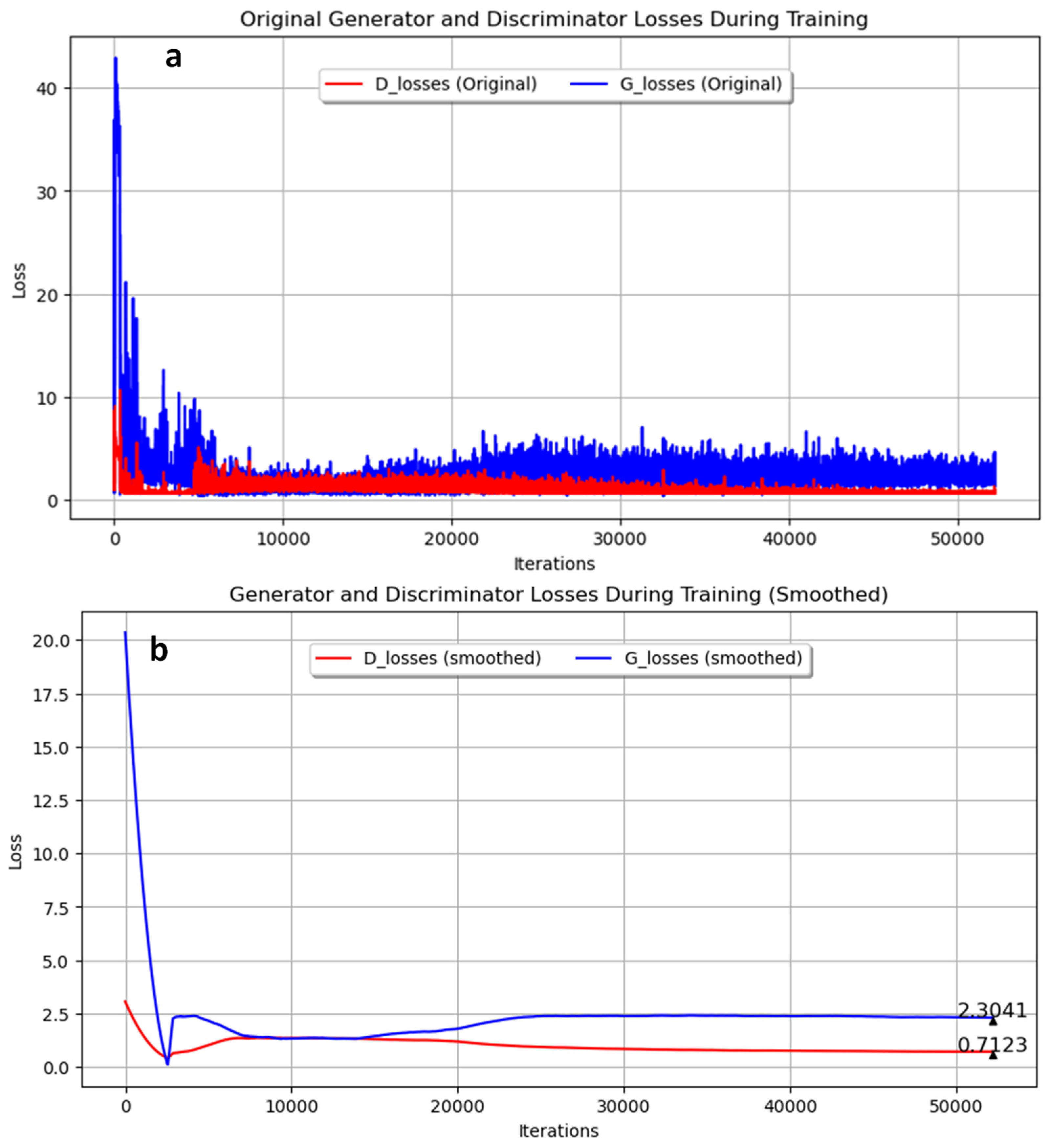
In the second experiment, the GAN was trained with annealed steel images for 300 epochs, using a filter size of 16 and a batch size of 8. The training progress is shown in Figure 6. Figure 6a presents the original training data, while Figure 6b shows the smoothed data. The final smoothed loss values were 2.3041 for the generator and 0.7123 for the discriminator. Similar to Experiment 1, the generator’s loss remained higher than the discriminator’s loss throughout the training process, indicating active learning in both networks. However, a different batch size of 8 was used in this experiment, compared to 4 in Experiment 1.

Figure 6.
Loss during training for pearlite and ferrite image generation over 300 epochs with 16 filters and mini-batch size of 8. (a) Original; (b) Smoothed.
Figure 7 displays the probability metrics D(G(z1)) and D(G(z2)). In this plot, D(G(z1)) is represented in red and D(G(z2)) in blue. As in Experiment 1, D(G(z1)) was consistently higher than D(G(z2)), with final values of 0.1223 and 0.0863, respectively. This indicates that the discriminator found it easier to identify images generated from z2 as synthetic compared to those from z1. The persistent challenge for the generator in producing indistinguishable images from the discriminator’s perspective is highlighted here as well.
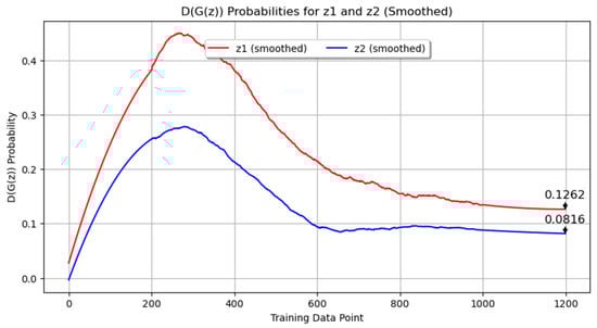
Figure 7.
Probability metrics D(G(z1)) and D(G(z2)) for Experiment 2.
Figure 8a compares a real image with images generated from Experiment 1, Figure 8b, and Experiment 2, Figure 8c. While the probability metrics indicated learning in both experiments, the visual comparison reveals that the quality of the generated images varies and may require more epochs for significant improvement.
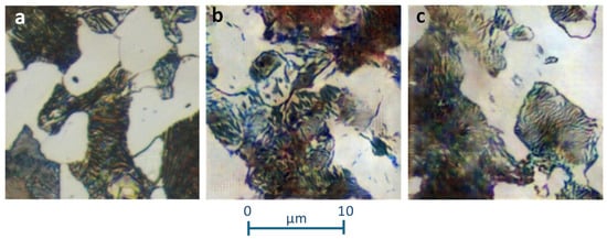
Figure 8.
Comparison of real and generated images of C45E steel from Experiments 1 and 2. (a) Real image and (b,c) synthetic images of Experiments 1 and 2, respectively.
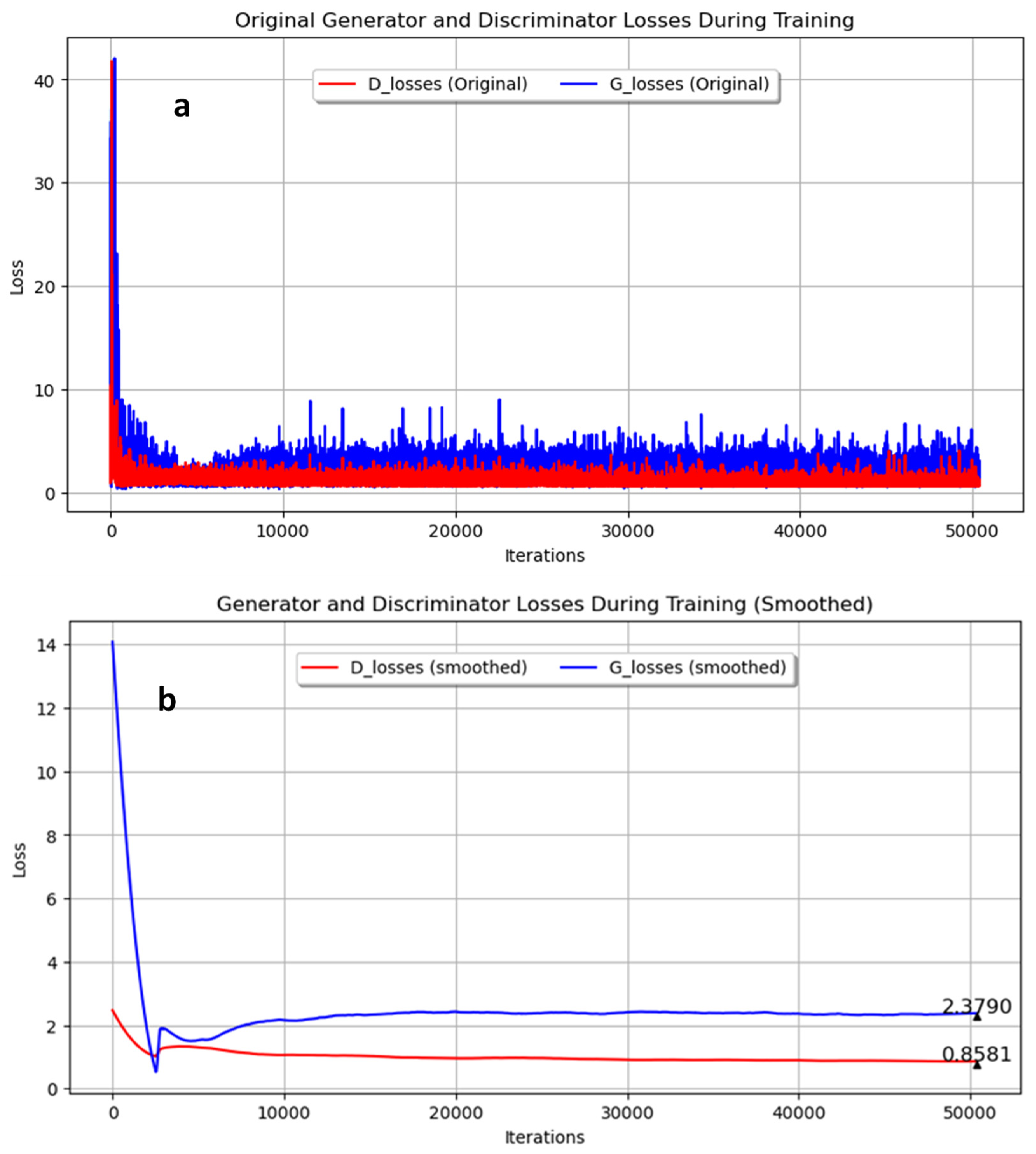
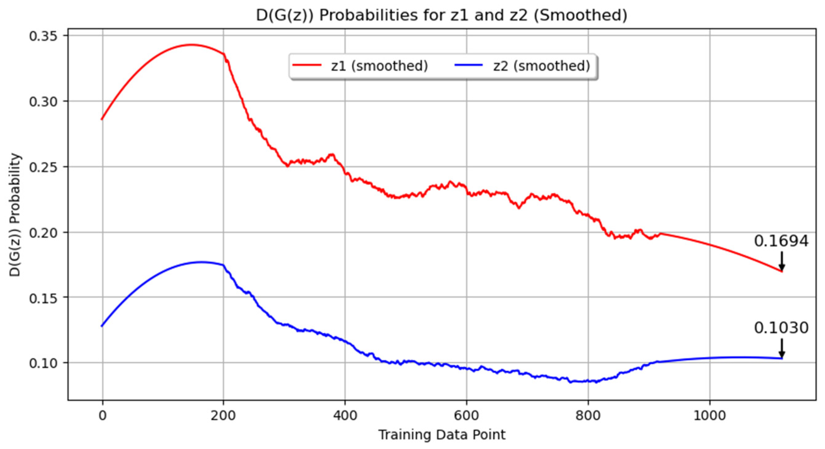
An additional experiment was conducted to generate images with the microconstituent martensite, originally produced in quenched samples together with the Widmanstätten structure. Figure 9 shows the evolution of the loss during training for both the generator and discriminator networks, with the original data and the smoothed data. The final smoothed loss values were 2.3790 for the generator and 0.8581 for the discriminator. These results suggest a balanced adversarial game, as the trends in the losses of the generator and discriminator were close to each other, indicating that both networks were improving concurrently and maintaining stable training dynamics. Figure 10 displays the smoothed probability metrics D(G(z1)) and D(G(z2)), which followed a similar trend to previous experiments, with final values of 0.1694 and 0.1030, respectively. Figure 11 presents a comparison between real and synthetic images. Despite the reduction in epochs, the generated images still demonstrated a high level of detail. While some blurry areas are present, the lamellar regions of pearlite and clear areas of ferrite are distinguishable, showing an acceptable level of detail for consideration as a microstructure resulting from the quenching process of low-carbon steel.
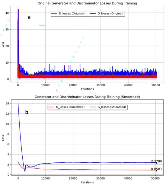
Figure 9.
Training progress of generator and discriminator losses for Experiment 3. (a) Original; (b) Smoothed.
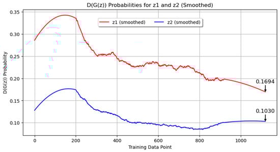
Figure 10.
Smoothed probability metrics D(G(z1)) and D(G(z2)) for Experiment 3.

Figure 11.
Comparison of real and synthetic images for Experiment 3. (a) real; (b) synthetic.
To contrast the previous results, other commonly used metrics in image generation were employed. The metrics used for evaluation were calculated using a script that measures inception score, Frechet inception distance (FID), and kernel inception distance (KID). The script utilizes a pre-trained Inception v3 model to extract features from real and generated images, then computes these metrics to assess the quality and diversity of the generated images. The results of these metrics are shown in Table 5 and are analyzed in detail in the Discussion section.
Table 5.
Evaluation metrics for Experiments 1, 2, and 3.
Additional images are provided in the Appendix A to enhance the understanding and perception of the results. Figure A1, Figure A2 and Figure A3 show the synthetic images produced in Experiments 1, 2, and 3, respectively, involving annealed steel in the first two experiments and quenched steel in the third. The hyperparameters used in each experiment are detailed in the figure captions. These visual representations provide an additional layer of validation for the effectiveness and variability of the GAN models under different training conditions.
4. Discussion
Our experiments with the GAN architecture yielded several valuable insights into the training dynamics and the impact of various hyperparameters on the quality of generated images. Initially, we started with 128 filters and 300 epochs, but this configuration resulted in out-of-memory errors. We observed that decreasing the batch size significantly improved the results. Furthermore, increasing the number of epochs up to the memory limit also enhanced image quality. Higher batch sizes, starting from sixteen, deteriorated the quality of the generated images, whereas a batch size of eight significantly enhanced image quality, leading us to conclude that lower batch sizes improve the results. Testing with eight filters showed a decline in performance compared to using sixteen filters. We also found that increasing the number of filters can improve the results, but there is a limitation due to the memory capacity of the device. Therefore, a trade-off must be reached between the number of filters, epochs, and memory to obtain the best images. Ultimately, the optimal configuration was found to be 400 epochs, 16 filters, and a batch size of 4, which yielded the best results. These findings suggest that larger batch sizes and higher filter counts negatively impact the quality of the generated images, likely due to the limitations of the GPU memory, which may not efficiently handle these larger configurations. Throughout the experiments, several key observations were made regarding the adversarial game between the generator and discriminator, the significance of the probability metrics D(G(z1)) and D(G(z2)), and the visual quality of the generated images.
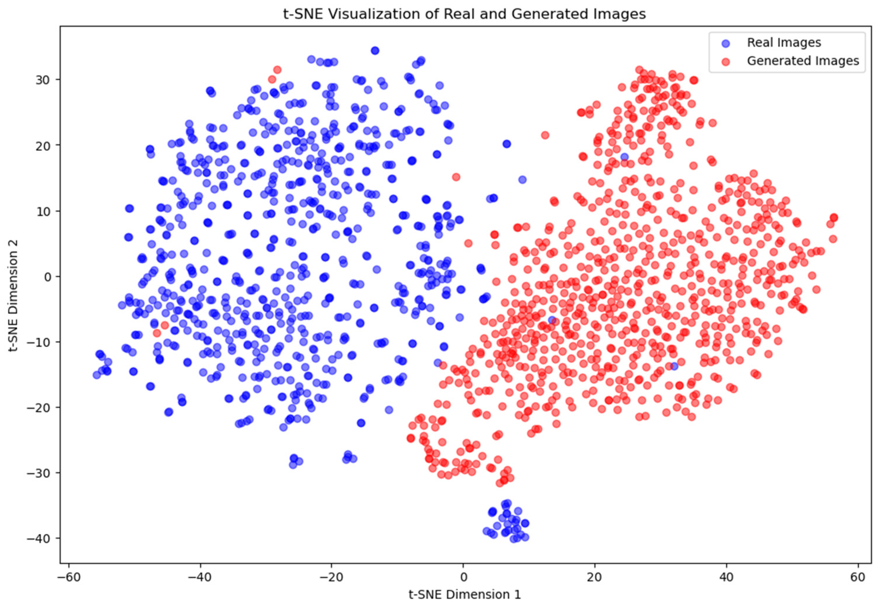
The t-SNE [38] plots generated for each experiment reveal distinct patterns in the distribution of features from the training and generated images. For Experiment 1, the t-SNE plot (Figure 12) shows that the points representing the training images, indicated by blue dots, and the points representing the generated images, indicated by red dots, are clearly separated. This clear separation indicates that the features extracted from the generated images were significantly different from those of the training images, suggesting that the generator was not able to replicate the training data distribution effectively.
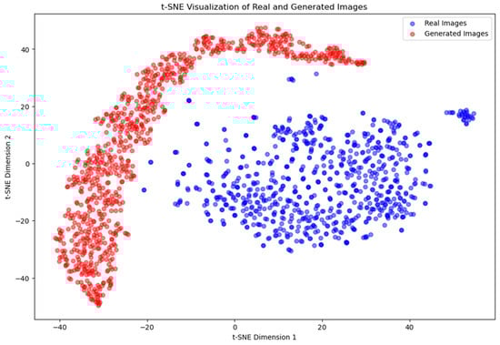
Figure 12.
t-SNE visualization of real and synthetic images for Experiment 1.
Similarly, in Experiment 3, the t-SNE plot (Figure 13) exhibits a clear separation between the points representing the training images and the generated images, with no overlap. The generated images again form an elongated and curved shape, with a noticeable spread among the points. This reinforces the observation that the generator was not able to capture the underlying data distribution of the training images sufficiently well. This can be justified by the high heterogeneity included in the image set of the Widmanstätten structure, which has been critical in generating latent variables during the computing process, resulting in no good results.
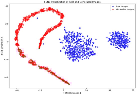
Figure 13.
t-SNE visualization of real and generated images for Experiment 3.
In Experiment 2, while the separation between the two groups remains, the clusters are somewhat closer to each other compared to Experiments 1 and 3. This slight reduction in distance, as shown in the t-SNE plot (Figure 14), suggests a marginal improvement in the generator’s ability to approximate the training data distribution. Despite this, the generated images are still not convincingly similar to the training images based on the feature distribution. However, they appear visually convincing at first glance, indicating that the generator is making progress in producing realistic images, even though it has not yet fully captured the underlying feature distribution.

Figure 14.
t-SNE visualization of real and generated images for Experiment 2.
From the perspective of GANs, the clear separation between the real and generated image features in the t-SNE plots indicates suboptimal performance of the generator. Ideally, for high-quality GAN training, the features of generated images should overlap significantly with those of the training images, reflecting that the generator has learned to produce images that are indistinguishable from the real ones. The observed separation suggests that, despite extensive experimentation and optimization of hyperparameters, the GAN’s training has not fully captured the complexities of the training data. These results represent the best performance achieved under the current experimental conditions, indicating that further advancements may require novel approaches or significant changes to the model architecture.
4.1. Training Dynamics and Loss Metrics
In Experiment 1, with annealed steel images trained for 350 epochs, it was observed that the generator’s loss was consistently higher than the discriminator’s loss. This indicates that the generator was struggling to produce images that the discriminator could not easily identify as synthetic. However, the proximity of the losses suggested that both networks were actively learning and improving. The use of the Savitzky–Golay filter to smooth the loss curves provided clearer insights into the overall trends, revealing a balanced adversarial game where neither network was overpowering the other.
Similarly, in Experiment 2, with annealed steel images trained for 300 epochs and a larger batch size of 8, the results indicated a persistent challenge for the generator. The final smoothed loss values showed a similar pattern to Experiment 1, reinforcing the importance of monitoring both the original and smoothed data to understand the training progress fully.
4.2. Probability Metrics
The probability metrics D(G(z1)) and D(G(z2)) provided additional qualitative insights into the discriminator’s ability to distinguish real images from generated ones. In both Experiment 1 and Experiment 2, D(G(z1)) remained consistently higher than D(G(z2)), indicating that the discriminator found it easier to identify images generated from z2 as synthetic compared to those from z1. These metrics are crucial for understanding the nuanced performance of the discriminator beyond simple loss values, highlighting specific challenges the generator faces in different stages of training.
In Experiment 3, conducted with quenched carbon steel images, the number of training images was increased, which exceeded the GPU memory capacity and required adjustments in training parameters. Despite these adjustments, the generated images demonstrated a high level of detail, indicating effective learning within the given constraints. The final smoothed probability values of D(G(z1)) and D(G(z2)) were 0.1694 and 0.1030, respectively, following a similar trend to previous experiments.
4.3. Additional Metrics
In this section, we analyze the results obtained from the additional evaluation metrics: inception score (IS), Frechet inception distance (FID), and kernel inception distance (KID). These metrics provide a quantitative assessment of the quality and diversity of the generated images, offering insights beyond the qualitative probability metrics D(G(z1)) and D(G(z2)).
The inception score measures both the quality and diversity of generated images, with higher scores indicating better performance. In our experiments, the IS varied significantly. Experiment 1 scored 1.373 ± 0.015, Experiment 2 scored 2.391 ± 0.152, and Experiment 3 scored 1.673 ± 0.049. The highest score in Experiment 2 suggests that the images generated were more diverse and of higher quality compared to the other experiments. This improvement is likely due to the adjustment in batch size, which provided a more stable training process.
Frechet inception distance measures the distance between feature distributions of real and generated images, with lower scores indicating better alignment with real image distributions. Experiment 1 had an FID score of 1124.113, Experiment 2 scored 456.309, and Experiment 3 scored 686.987. These scores indicate that Experiment 2 produced images closest in distribution to the real images, followed by Experiment 3, while Experiment 1 had the highest divergence. This finding aligns with the inception score results, reinforcing that the changes in training parameters for Experiment 2 positively impacted generative quality.
The Kernel inception distance also measures similarity between real and generated image distributions, with lower scores indicating better performance. The KID scores were 3.350 for Experiment 1, 2.153 for Experiment 2, and 3.012 for Experiment 3. Similar to the FID results, the KID indicates that Experiment 2 had the best performance, suggesting more effective learning and generation of images closely resembling the real ones.
The additional metrics provide a comprehensive evaluation of the GAN’s performance. Experiment 2 consistently showed the best results across all metrics, indicating that the adjustments made to the training parameters were effective for the training dataset.
4.4. Visual Quality of Generated Images
While the t-SNE plots, probability metrics, and loss values provide additional quantitative measures of the GAN’s performance, the visual quality of the generated images is highly important. The comparison between real and generated images in Figure 8 and Figure 11 reveals distinct outcomes for different experiments. In Experiments 1 and 2, the generated images captured essential microstructural details such as lamellar regions of pearlite and clear areas of ferrite, which closely resemble the microstructures of annealed carbon steel as recognized by metallurgy experts. However, in Experiment 3, the generated images of martensite presented some doubts when viewed by experts. Although they demonstrated a high level of detail, the images were not as convincingly realistic as those from the annealed steel experiments. These qualitative observations suggest that, despite the metrics, the visual inspection by experts reveals a nuanced understanding of the GAN’s performance, highlighting areas where the generated images align well with expected microstructures and where they fall short. Really, what happens is that some synthetic microstructures are unreal, as they combine constituents that are not compatible with steel after a quenching treatment, i.e., ferrite and martensite.
5. Conclusions
The experiments highlight the importance of a balanced adversarial game between the generator and discriminator to achieve stable training dynamics and high-quality image generation. The use of smoothed loss curves and probability metrics provides deeper insights into the training process, beyond what is visible from raw data alone. Future work could explore optimizing hyperparameters further, using advanced techniques such as Wasserstein GANs (WGANs) with gradient penalty (GP) [39], as well as addressing hardware limitations to enable longer training periods and larger batch sizes [40].
Overall, the results demonstrate the potential of GANs in generating realistic microstructures for materials science applications, provided that careful attention is given to both quantitative metrics and visual quality assessments. The experiments with annealed steel images showed promising results, closely aligning with expert expectations for annealed carbon steel microstructures, while the experiment with martensite highlighted areas for further improvement in generating highly convincing microstructures under constrained training conditions.
Importantly, these generation experiments are not merely exercises in image synthesis. They are crucial for new image generation and data augmentation, which are valuable for subsequent analyses and applications. This research is particularly significant because it allows us to expand the image database, which is a critical bottleneck in this field. By increasing the database, models can be continuously developed to update and enhance previous research on classification and segmentation. Additionally, the understanding of the physical properties of steels based on the observation of microstructures will be advanced, which will be a future line of investigation.
Moreover, progress is aimed at creating synthetic microstructural images that can be tailored according to the microconstituent of interest, with custom-made images of high educational value being generated. Overall, the potential of GANs as powerful tools for materials science is highlighted by this study, provided that both quantitative and qualitative aspects are carefully managed. By generating realistic microstructures, materials development can be accelerated, processing conditions optimized, and new material compositions explored more efficiently.
Author Contributions
Conceptualization, J.M.-R., F.G.-S. and V.M.-E.; methodology, J.M.-R., F.G.-S., J.C.-S., A.M.-M. and V.M.-E.; software, J.M.-R. and F.G.-S.; validation, J.C.-S., A.M.-M. and J.M.-R.; formal analysis, J.M.-R., F.G.-S. and V.M.-E.; investigation, J.M.-R., A.M.-M. and J.C.-S.; resources, A.M.-M., J.C.-S., F.G.-S. and V.M.-E.; data curation, J.M.-R. and F.G.-S.; writing—original draft preparation, J.M.-R.; writing—review and editing, J.M.-R., F.G.-S. and V.M.-E.; visualization, F.G.-S. and V.M.-E.; supervision, F.G.-S., J.C.-S., A.M.-M. and V.M.-E.; All authors have read and agreed to the published version of the manuscript.
Funding
This research did not receive any specific grant from funding agencies in the public, commercial, or not-for-profit sectors.
Institutional Review Board Statement
Not applicable.
Informed Consent Statement
Not applicable.
Data Availability Statement
Data are contained within the article.
Conflicts of Interest
The authors declare no conflicts of interest.
Appendix A
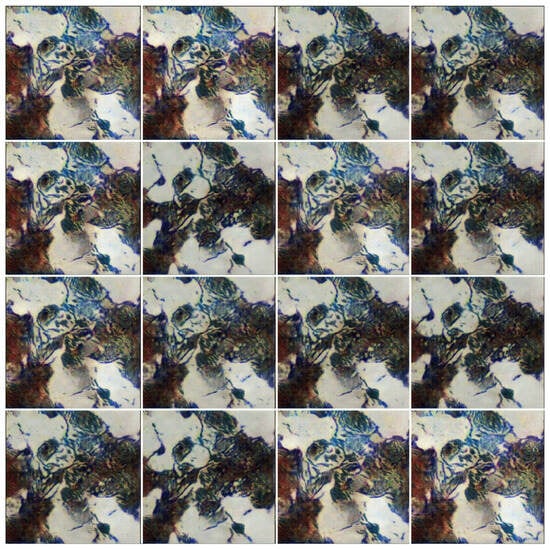
Figure A1.
Experiment 1: Annealed steel synthetic images. Hyperparameters: epochs = 350, learning rate = 0.0002, number of filters = 16, kernel size = 4, batch size = 4.
Figure A1.
Experiment 1: Annealed steel synthetic images. Hyperparameters: epochs = 350, learning rate = 0.0002, number of filters = 16, kernel size = 4, batch size = 4.
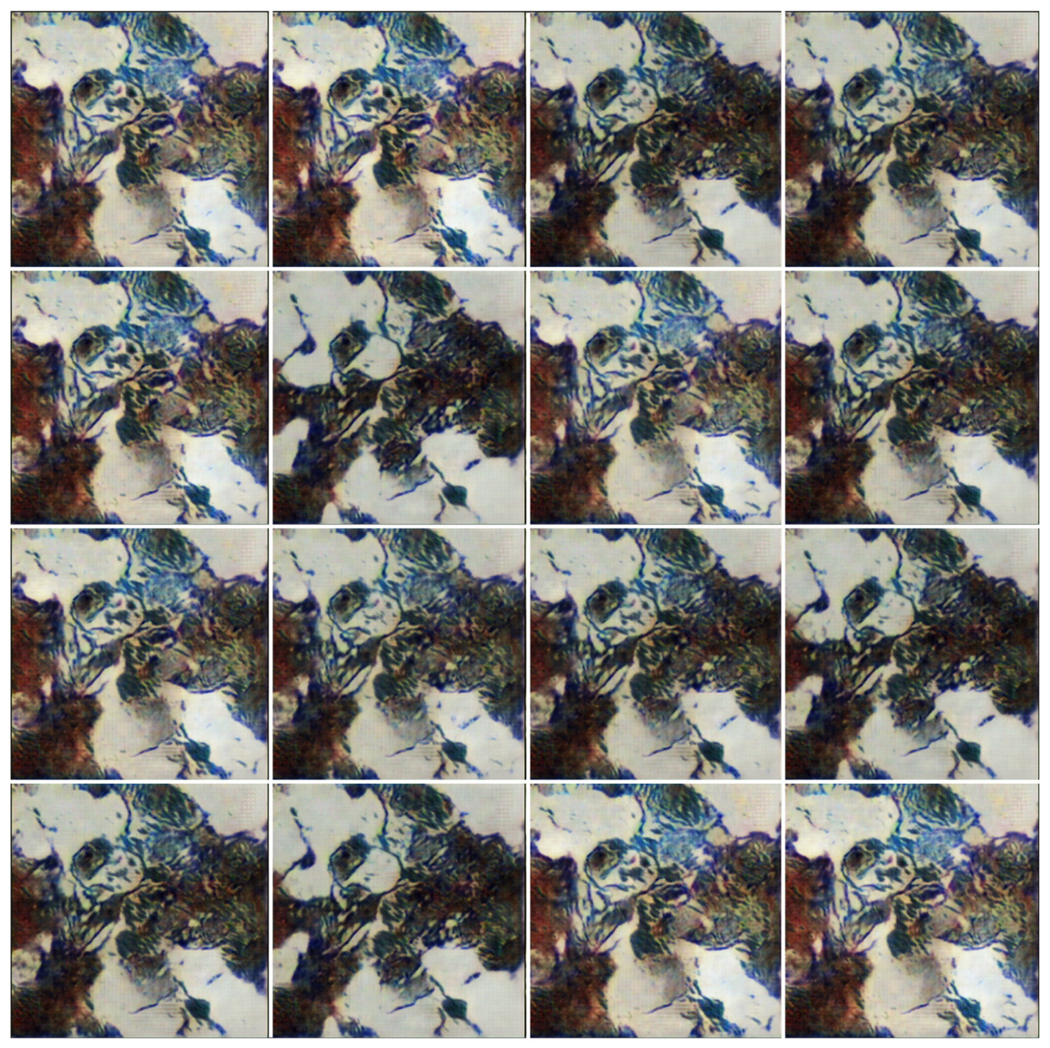
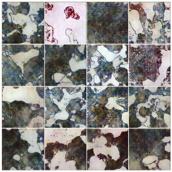
Figure A2.
Experiment 2: Annealed steel synthetic images. Hyperparameters: epochs = 300, learning rate = 0.0002, number of filters = 16, kernel size = 4, batch size = 8.
Figure A2.
Experiment 2: Annealed steel synthetic images. Hyperparameters: epochs = 300, learning rate = 0.0002, number of filters = 16, kernel size = 4, batch size = 8.

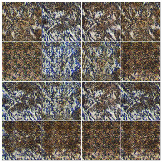
Figure A3.
Experiment 3: Quenched steel synthetic images. Hyperparameters: epochs = 300, learning rate = 0.0002, number of filters = 16, kernel size = 4, batch size = 8.
Figure A3.
Experiment 3: Quenched steel synthetic images. Hyperparameters: epochs = 300, learning rate = 0.0002, number of filters = 16, kernel size = 4, batch size = 8.

References
- Torquato, S.; Haslach, H.W. Random Heterogeneous Materials: Microstructure and Macroscopic Properties. Appl. Mech. Rev. 2002, 55, B62–B63. [Google Scholar] [CrossRef]
- Kamrava, S.; Tahmasebi, P.; Sahimi, M. Linking Morphology of Porous Media to Their Macroscopic Permeability by Deep Learning. Transp. Porous Media 2020, 131, 427–448. [Google Scholar] [CrossRef]
- Cang, R.; Li, H.; Yao, H.; Jiao, Y.; Ren, Y. Improving Direct Physical Properties Prediction of Heterogeneous Materials from Imaging Data via Convolutional Neural Network and a Morphology-Aware Generative Model. Comput. Mater. Sci. 2018, 150, 212–221. [Google Scholar] [CrossRef]
- Yabansu, Y.C.; Altschuh, P.; Hötzer, J.; Selzer, M.; Nestler, B.; Kalidindi, S.R. A Digital Workflow for Learning the Reduced-Order Structure-Property Linkages for Permeability of Porous Membranes. Acta Mater. 2020, 195, 668–680. [Google Scholar] [CrossRef]
- Yang, Z.; Yabansu, Y.C.; Jha, D.; Liao, W.-K.; Choudhary, A.N.; Kalidindi, S.R.; Agrawal, A. Establishing Structure-Property Localization Linkages for Elastic Deformation of Three-Dimensional High Contrast Composites Using Deep Learning Approaches. Acta Mater. 2019, 166, 335–345. [Google Scholar] [CrossRef]
- Jiao, Y.; Stillinger, F.H.; Torquato, S. A Superior Descriptor of Random Textures and Its Predictive Capacity. Proc. Natl. Acad. Sci. USA 2009, 106, 17634–17639. [Google Scholar] [CrossRef]
- Choudhary, K.; DeCost, B.; Chen, C.; Jain, A.; Tavazza, F.; Cohn, R.; Park, C.W.; Choudhary, A.; Agrawal, A.; Billinge, S.J.L.; et al. Recent Advances and Applications of Deep Learning Methods in Materials Science. Npj Comput. Mater. 2022, 8, 59. [Google Scholar] [CrossRef]
- Muntin, A.V.; Zhikharev, P.Y.; Ziniagin, A.G.; Brayko, D.A. Artificial Intelligence and Machine Learning in Metallurgy. Part 1. Methods and Algorithms. Metallurgist 2023, 67, 886–894. [Google Scholar] [CrossRef]
- Pan, G.; Wang, F.; Shang, C.; Wu, H.; Wu, G.; Gao, J.; Wang, S.; Gao, Z.; Zhou, X.; Mao, X. Advances in Machine Learning- and Artificial Intelligence-Assisted Material Design of Steels. Int. J. Miner. Metall. Mater. 2023, 30, 1003–1024. [Google Scholar] [CrossRef]
- Agrawal, A.; Choudhary, A. Deep Materials Informatics: Applications of Deep Learning in Materials Science. MRS Commun. 2019, 9, 779–792. [Google Scholar] [CrossRef]
- Alrfou, K.; Kordijazi, A.; Zhao, T. Computer Vision Methods for the Microstructural Analysis of Materials: The State-of-the-Art and Future Perspectives. arXiv 2022, arXiv:2208.04149. [Google Scholar]
- Goodfellow, I.J.; Pouget-Abadie, J.; Mirza, M.; Xu, B.; Warde-Farley, D.; Ozair, S.; Courville, A.; Bengio, Y. Generative Adversarial Networks. arXiv 2014, arXiv:1406.2661. [Google Scholar] [CrossRef]
- Iyer, A.; Dey, B.; Dasgupta, A.; Chen, W.; Chakraborty, A. A Conditional Generative Model for Predicting Material Microstructures from Processing Methods. arXiv 2019, arXiv:1910.02133. [Google Scholar]
- DeCost, B.L.; Lei, B.; Francis, T.; Holm, E.A. High Throughput Quantitative Metallography for Complex Microstructures Using Deep Learning: A Case Study in Ultrahigh Carbon Steel. Microsc. Microanal. 2019, 25, 21–29. [Google Scholar] [CrossRef]
- Bostanabad, R. Reconstruction of 3D Microstructures from 2D Images via Transfer Learning. Comput.-Aided Des. 2020, 128, 102906. [Google Scholar] [CrossRef]
- Li, X.; Zhang, Y.; Zhao, H.; Burkhart, C.; Brinson, L.C.; Chen, W. A Transfer Learning Approach for Microstructure Reconstruction and Structure-Property Predictions. Sci. Rep. 2018, 8, 13461. [Google Scholar] [CrossRef]
- Shams, R.; Masihi, M.; Boozarjomehry, R.B.; Blunt, M.J. Coupled Generative Adversarial and Auto-Encoder Neural Networks to Reconstruct Three-Dimensional Multi-Scale Porous Media. J. Pet. Sci. Eng. 2020, 186, 106794. [Google Scholar] [CrossRef]
- Cang, R.; Xu, Y.; Chen, S.; Liu, Y.; Jiao, Y.; Yi Ren, M. Microstructure Representation and Reconstruction of Heterogeneous Materials Via Deep Belief Network for Computational Material Design. J. Mech. Des. 2017, 139, 071404. [Google Scholar] [CrossRef]
- Saxena, D.; Cao, J. Generative Adversarial Networks (GANs): Challenges, Solutions, and Future Directions. ACM Comput. Surv. 2022, 54, 63. [Google Scholar] [CrossRef]
- Mosser, L.; Dubrule, O.; Blunt, M.J. Stochastic Reconstruction of an Oolitic Limestone by Generative Adversarial Networks. Transp. Porous Media 2018, 125, 81–103. [Google Scholar] [CrossRef]
- Mosser, L.; Dubrule, O.; Blunt, M.J. Reconstruction of Three-Dimensional Porous Media Using Generative Adversarial Neural Networks. Phys. Rev. E 2017, 96, 043309. [Google Scholar] [CrossRef] [PubMed]
- Singh, R.; Shah, V.; Pokuri, B.; Sarkar, S.; Ganapathysubramanian, B.; Hegde, C. Physics-Aware Deep Generative Models for Creating Synthetic Microstructures. arXiv 2018, arXiv:1811.09669. [Google Scholar]
- Yang, Z.; Li, X.; Catherine Brinson, L.; Choudhary, A.N.; Chen, W.; Agrawal, A. Microstructural Materials Design Via Deep Adversarial Learning Methodology. J. Mech. Des. 2018, 140, 111416. [Google Scholar] [CrossRef]
- Xiao, S.; Bordas, S.P.A.; Kim, T.-Y. Editorial: Deep Learning in Computational Materials Science. Front. Mater. 2023, 10, 1198344. [Google Scholar] [CrossRef]
- Lee, J.-W.; Goo, N.H.; Park, W.B.; Pyo, M.; Sohn, K.-S. Virtual Microstructure Design for Steels Using Generative Adversarial Networks. Eng. Rep. 2021, 3, e12274. [Google Scholar] [CrossRef]
- Thakre, S.; Karan, V.; Kanjarla, A.K. Quantification of Similarity and Physical Awareness of Microstructures Generated via Generative Models. Comput. Mater. Sci. 2023, 221, 112074. [Google Scholar] [CrossRef]
- Narikawa, R.; Fukatsu, Y.; Wang, Z.-L.; Ogawa, T.; Adachi, Y.; Tanaka, Y.; Ishikawa, S. Generative Adversarial Networks-based Synthetic Microstructures for Data-driven Materials Design. Adv. Theory Simul. 2022, 5, 2100470. [Google Scholar] [CrossRef]
- Sugiura, K.; Ogawa, T.; Adachi, Y. Hourly Work of 3D Microstructural Visualization of Dual Phase Steels by SliceGAN. Adv. Theory Simul. 2022, 5, 2200132. [Google Scholar] [CrossRef]
- Jabbar, R.; Jabbar, R.; Kamoun, S. Recent Progress in Generative Adversarial Networks Applied to Inversely Designing Inorganic Materials: A Brief Review. Comput. Mater. Sci. 2022, 213, 111612. [Google Scholar] [CrossRef]
- Muñoz-Ródenas, J.; Miguel, V.; García-Sevilla, F.; Coello, J.; Martínez-Martínez, A. Machine Learning Approaches for Classification of Ultra High Carbon Steel Micrographs. Key Eng. Mater. 2023, 959, 119–127. [Google Scholar] [CrossRef]
- Muñoz-Rodenas, J.; García-Sevilla, F.; Coello-Sobrino, J.; Martínez-Martínez, A.; Miguel-Eguía, V. Effectiveness of Machine-Learning and Deep-Learning Strategies for the Classification of Heat Treatments Applied to Low-Carbon Steels Based on Microstructural Analysis. Appl. Sci. 2023, 13, 3479. [Google Scholar] [CrossRef]
- Muñoz-Rodenas, J.; García-Sevilla, F.; Miguel-Eguía, V.; Coello-Sobrino, J.; Martínez-Martínez, A. A Deep Learning Approach to Semantic Segmentation of Steel Microstructures. Appl. Sci. 2024, 14, 2297. [Google Scholar] [CrossRef]
- Ma, B.; Wei, X.; Liu, C.; Ban, X.; Huang, H.; Wang, H.; Xue, W.; Wu, S.; Gao, M.; Shen, Q.; et al. Data Augmentation in Microscopic Images for Material Data Mining. Npj Comput. Mater. 2020, 6, 125. [Google Scholar] [CrossRef]
- Shorten, C.; Khoshgoftaar, T.M. A Survey on Image Data Augmentation for Deep Learning. J. Big Data 2019, 6, 60. [Google Scholar] [CrossRef]
- Radford, A.; Metz, L.; Chintala, S. Unsupervised Representation Learning with Deep Convolutional Generative Adversarial Networks. arXiv 2015, arXiv:1511.06434. [Google Scholar]
- Hinton, G.E. 20—CONNECTIONIST LEARNING PROCEDURES11. This Chapter Appeared in Volume 40 of Artificial Intelligence in 1989, Reprinted with Permission of North-Holland Publishing. It Is a Revised Version of Technical Report CMU-CS-87-115, Which Has the Same Title and Was Prepared in June 1987 While the Author Was at Carnegie Mellon University. The Research Was Supported by Contract N00014-86-K-00167 from the Office of Naval Research and by Grant IST-8520359 from the National Science Foundation. In Machine Learning; Kodratoff, Y., Michalski, R.S., Eds.; Morgan Kaufmann: San Francisco, CA, USA, 1990; pp. 555–610. ISBN 9780080510552. [Google Scholar]
- Savitzky, A.; Golay, M.J.E. Smoothing and Differentiation of Data by Simplified Least Squares Procedures. Anal. Chem. 1964, 36, 1627–1639. [Google Scholar] [CrossRef]
- Van der Maaten, L.; Hinton, G. Visualizing Data Using T-SNE. J. Mach. Learn. Res. 2008, 9, 2579–2605. [Google Scholar]
- Gulrajani, I.; Ahmed, F.; Arjovsky, M.; Dumoulin, V.; Courville, A. Improved Training of Wasserstein GANs. arXiv 2017, arXiv:1704.00028. [Google Scholar]
- Karras, T.; Aila, T.; Laine, S.; Lehtinen, J. Progressive Growing of GANs for Improved Quality, Stability, and Variation. arXiv 2017, arXiv:1710.10196. [Google Scholar]


Disclaimer/Publisher’s Note: The statements, opinions and data contained in all publications are solely those of the individual author(s) and contributor(s) and not of MDPI and/or the editor(s). MDPI and/or the editor(s) disclaim responsibility for any injury to people or property resulting from any ideas, methods, instructions or products referred to in the content. |
© 2024 by the authors. Licensee MDPI, Basel, Switzerland. This article is an open access article distributed under the terms and conditions of the Creative Commons Attribution (CC BY) license (https://creativecommons.org/licenses/by/4.0/).