New Physically-Based Mathematical Model and Experiments for a Recently Invented Solar Pot

Abstract

The studied solar pot is a recent invention, which is made for environmentally friendly cooking or heating (by utilizing solar energy) of foods and liquids. Its structure is similar to a double pipe heat exchanger, it has an outer mantle and an inner cooking tank. The goals of the paper are proposing a new physically-based mathematical model describing the solar pot and carrying out computer experiments with it, assembling an experimental system of the pot connected with a solar collector and performing measurements on it. Based on the results, the solar pot can successfully be used for cooking or sterilizing foods or liquids during the studied time period, in Hungary. In particular, based on measured data, the temperature level needed for heat treatment (75 °C) can be maintained in the cooking tank for several hours (~5 h, on the average) in a typical day in May.

1. Introduction

The thermal energy provided by the sun is used to treat food in different ways. Examples include drying [1], baking and cooking [2]. Solar food preparation devices operated with solar energy are known, in which solar energy directly heats a surface or air along it in a closed box, and the heat is transferred from there to the closed vessel placed in the box [3]. With this solution, the preparation of food by cooking cannot be solved in many cases [4]. However, there are solar cookers able to produce the temperature required for cooking, which is 73.9 °C according to [5]. Typical types are the reflective panel [6], the parabolic [7] and the evacuated tube solar cooker [8]. These are the so-called direct-type food processing devices. Indirect types use a solar collector to produce the thermal energy needed for food processing.

In [9] a solar cooker with solar collector and heat storage is investigated in China that uses oil as heat transfer medium. The main elements of the system are the solar collector, the heat storage and the cooking plate, which can be converted into a traditional electric cooking plate when supplemented with a heating element, enabling cooking even when there is not enough solar energy available. The main goal of the research was to investigate the effect of the quartzite heat storage medium on the system. For this, a mathematical model describing the performance of the system was prepared. The design with heat storage was compared with a version with one and two heat storage tanks. Based on the results, the version with quartzite heat storage increases the performance of the system, and the investment cost also decreases. The solar share was 71% which clearly means a significant reduction in the carbon dioxide emission with regard to the cooking activity. In the investigations of the present paper on a mantle-pot equipment that we call solar pot, working with only solar heat, the solar share is even higher, 100%. Nevertheless, the completion of the pot with some auxiliary heating may come into consideration in the future, as it is mentioned in the Conclusions. (It would decrease the solar share but increase the operating period of the pot.)

In [10] a research is conducted on an indirect type solar food processing device with nanofluid working medium. One of the main elements of the system is the parabolic solar collector, at the focal point of which the working medium is heated by flowing through it. The other important element is the cooking unit, which consists of a copper pot and the copper pipe that surrounds it (wrapped around it). The heated working medium flows in this pipe, thus transferring the heat to the cooking space. A separate tank was also installed between the cooking unit and the collector, through which the working medium also flows. Due to the parabolic collector, the spiral heat exchanger and the additional tank, the structure of the system is more complex and thus its implementation is obviously more expensive than the system of the solar pot of this paper, which uses a more conventional evacuated tube collector and the solar pot similar to a simple, jacketed heat exchanger. The authors investigated the effect of mixing nano-sized particles with the oil serving as the working medium, how the mass fraction of the particles and the volumetric flow rate of the medium affect the development of the system’s energy efficiency. The mass fraction was varied between 0 and 0.5% by mass, and the flow rate between 0.25 and 0.55 ${\displaystyle \frac{\mathrm{L}}{\mathrm{m}\mathrm{i}\mathrm{n}}}$. Based on their tests, it was found that while the efficiency of the collector increases continuously with the increase in volumetric flow rate, the highest efficiency is achieved in the case of the cooking unit at 0.25 ${\displaystyle \frac{\mathrm{L}}{\mathrm{m}\mathrm{i}\mathrm{n}}}$. Increasing the mass ratio increases the energy efficiency of both main units. The energy efficiency of the entire system increases by 20.08% in the case of a particle concentration of 0.5% by mass and a flow rate of 0.25 ${\displaystyle \frac{\mathrm{L}}{\mathrm{m}\mathrm{i}\mathrm{n}}}$, and 2 litres of water at 30 °C could be heated to boiling point in 31.51% less time as in the case of the version using oil only. In [11] an indirect-type solar cooker is prepared in Egypt with flat plate collectors equipped with reflectors. They used phase change material, magnesium nitrate hexahydrate, mixed with steel shavings as heat storage material. The equipment is capable of cooking general meals in the midday and afternoon hours. In the evening it can be used to prepare special dishes that can be cooked at low temperatures for a long time (e.g., beans). In the night and morning hours it can be used to keep or reheat food. In [12] it was investigated how the performance of the system changes when the collector is supplemented with reflectors in an indirect solar food processing system equipped with a flat plate collector with water as working medium and supplemented with a heat storage tank containing a phase change material. They found that without a reflector, the highest average temperature of the absorber is 92 °C, the highest temperature of the outlet working medium is 71 °C, and the highest energy efficiency is 63%. It can be stated that the system is not suitable for cooking as the minimum safe temperature for cooking is 73.9 °C according to [5]. On the other hand, thanks to the addition of reflectors, these values were respectively 130 °C, 103.65 °C and 79%. The device was used to cook 1 kg of rice and 1 kg of pasta in 1.5 L of water. In both cases they were successful. It should be mentioned that the additions made in order to increase the performance of the equipment significantly increased the complexity of the system. The system examined in this paper has a simpler design and does not contain phase change material. In [13] a solar pressure cooker is investigated, which is connected to an evacuated tube solar collector to provide the necessary energy for operation. The water heated in the collector flows directly into the cooking chamber (under pressure) without the intervention of a heat exchanger. Thus, during operation, the condition of the heat-treated raw material/food must be difficult to check. The system we are examining is more practical, the cooking space is accessible during operation too, as it is hydraulically separated from the collector circuit under pressure. In [13] they used experiments to investigate the thermal behaviour of the equipment, under different weather conditions (radiation intensity, ambient temperature), regarding the boiling of different masses of water. Based on their results, a larger mass of water boils proportionally in less time, so the efficiency of the system improves when larger quantities are boiled. In [14] a large-scale cooking system was made capable of supplying energy to several cooking units at the same time. The flat plate collector system also includes a heat storage tank made of oil and stone, in addition to the cooking units. The flow of the working medium is not forced, no pump is needed. The system has been successfully used for food preparation in several developing countries (e.g., Mali, India). The system, that is the subject of this paper’s research, works with a pump, so its placement/implementation can be done in a less constrained manner, it is also simpler and does not contain heat storage.

The main elements of the system examined in this paper are the solar collector and the so-called solar pot. In the literature, there are mathematical models for collectors and solar heating systems [15,16], however, as it is a new invention, no model has yet been worked out for the solar pot. In terms of design, the solar pot is similar to a tube-in-tube heat exchanger or a solar storage tank. Models for those are already available in the literature. There are two main types of models. One is the black-box type and the other one is the physically-based model. The physically-based model relies on the physical background of the modelled system or process, which is therefore often difficult to set up in the case of a complex system [17]. Black-box modelling does not take into account the physical background, it represents a more result-oriented approach, the creation of the model is typically simpler [18,19].

The Hottel-Whillier-Bliss physically-based mathematical model worked out for flat plate collectors [20] can be used to describe the temperature distribution of the working medium along the length of the collector as a function of place and time. In [21] a physically-based mathematical model was developed that can be used to describe the temporal behaviour of a flat plate collector. Estimation of the temperature of the outlet working medium is made possible by a differential equation formulated on the basis of the energy balance of the collector. Reference [22] presents several physically-based mathematical models describing the dynamic behaviour of unglazed flat plate collectors. In [23] the possibility of a device that can be used for heating and domestic hot water production was developed, in which the collector is equipped with a mirror. In connection with this, a physically-based model was worked out for evacuated tube solar collectors, which can be used to estimate the total solar radiation reaching the collector. In [24] a black-box type neural network model was made, which can be used to model the thermal behaviour of a flat plate collector. Knowing the intensity of solar radiation, the ambient temperature and the temperature of the working medium entering the collector, with a constant mass flow, the temperature of the outlet heat transfer medium can be predicted with the model. In [25] a black-box model based on multiple linear regression was developed for solar collectors. As a result, the appropriate temperature of the outlet working medium can be calculated. The identified and validated model was compared to the physically-based model of [21]. The results showed that the model in [25] was able to predict the temperature of the outlet working medium more accurately. The importance of the model, in addition to the appropriate accuracy (average accuracy better than 5%), is due to its simplicity. It requires little calculation and can be used for any type of collector (e.g., evacuated tube collector).

There are several mixed storage models in the literature. In [15] a physically-based mathematical model was developed. An ordinary differential equation based on the energy balance of the tank allows the temperature of the tank to be calculated. The model does not take into account the heat capacity of the solar storage material. In [26] a physically-based mathematical model for a mixed storage was worked out, based on the heat balance of the storage, which can be used to calculate the temperature of the storage. A similar model can be found in [27]. In [28] a black-box model based on multiple linear regression was developed for mixed solar storages, which can be used to determine the geometric average temperature of the storage.

When modelling tube-in-tube heat exchangers, energy balance is often assumed between the working media of the two sides, neglecting the environmental heat exchange [29,30]. In [31] various mathematical models for tube-in-tube heat exchangers similar to the solar pot examined in this paper were developed. The physically-based model takes into account the heat exchange with the environment, too. A black-box type mathematical model was also developed in [31] based on multiple linear regression, which also takes environmental heat exchange into account. The models were validated using measurements on a heat exchanger. Based on the results, the physically-based model not neglecting the heat exchange with the environment can estimate the temperature of the outlet working medium more accurately than the other model version assuming energy balance between the two sides of a heat exchanger. The black-box model proved to be more accurate than both models, in case of considerable environmental heat exchange. In [32] there are physically-based models for tube-in-tube heat exchangers. The first one is a model with distributed parameters, which can be used to calculate the temperature of the working medium on the cold and hot sides of the heat exchanger. The second one is a second-order concentrated parameter model, which can be used to determine the outlet temperature of the cold and hot side working fluids. According to the authors’ conclusion, second-order concentrated parameter models based on the logarithmic mean temperature difference approach can reliably describe the dynamics of heat exchangers.

The contribution of the present paper is as follows:

• A new physically-based mathematical model is proposed to describe the examined, recently invented solar pot. Computer simulations are made with the model, based on which conclusions are drawn regarding the practical applicability of the solar pot.
• An experimental system of the hydraulically connected solar pot and a solar collector is physically assembled. The different variables of the system (different temperature values) are measured. Based on measured data, conclusions are drawn regarding the practical applicability of the solar pot.

The structure of the paper is the following: Section 2 contains the description of the modelled and measured system. Section 3 presents the physically-based model of the solar pot along with the simulation results. In Section 4, the measurements made on the experimental system and the measured data are shown. Section 5 serves with conclusions and future research proposals.

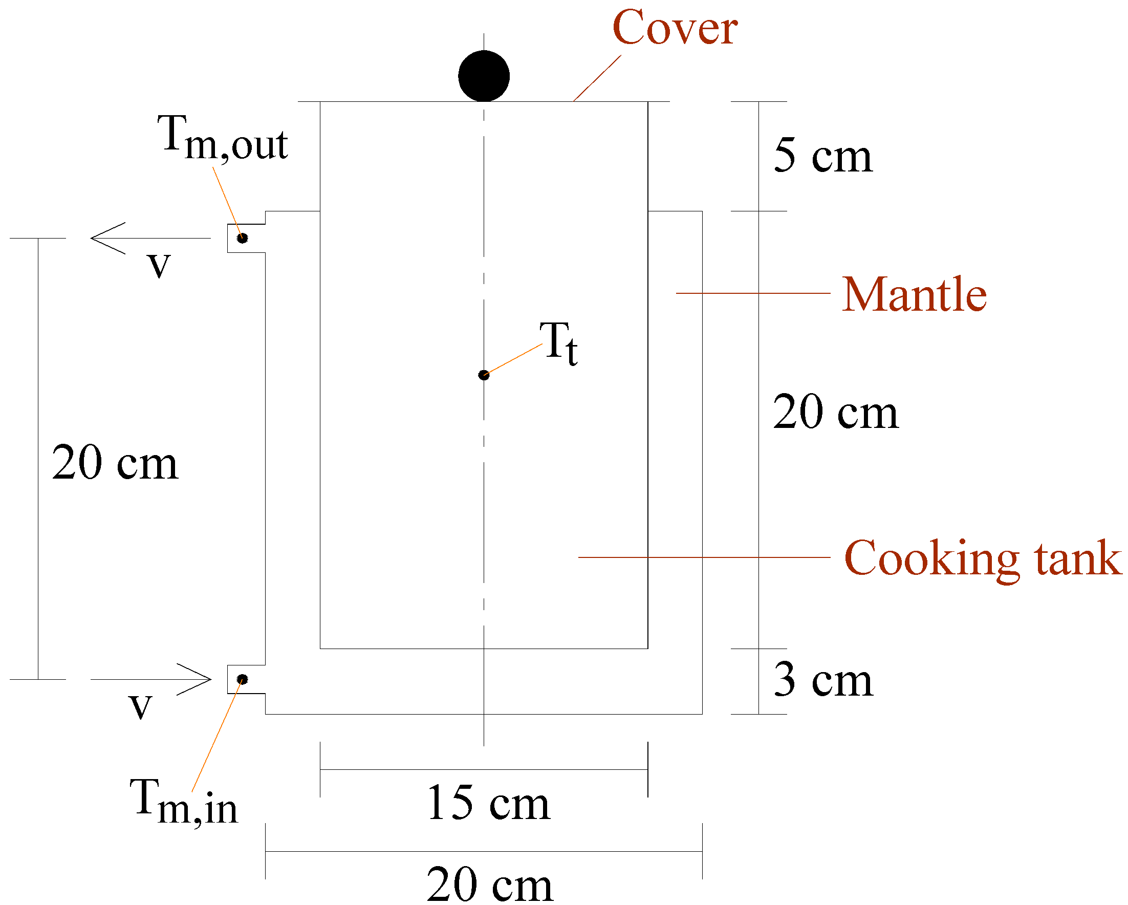
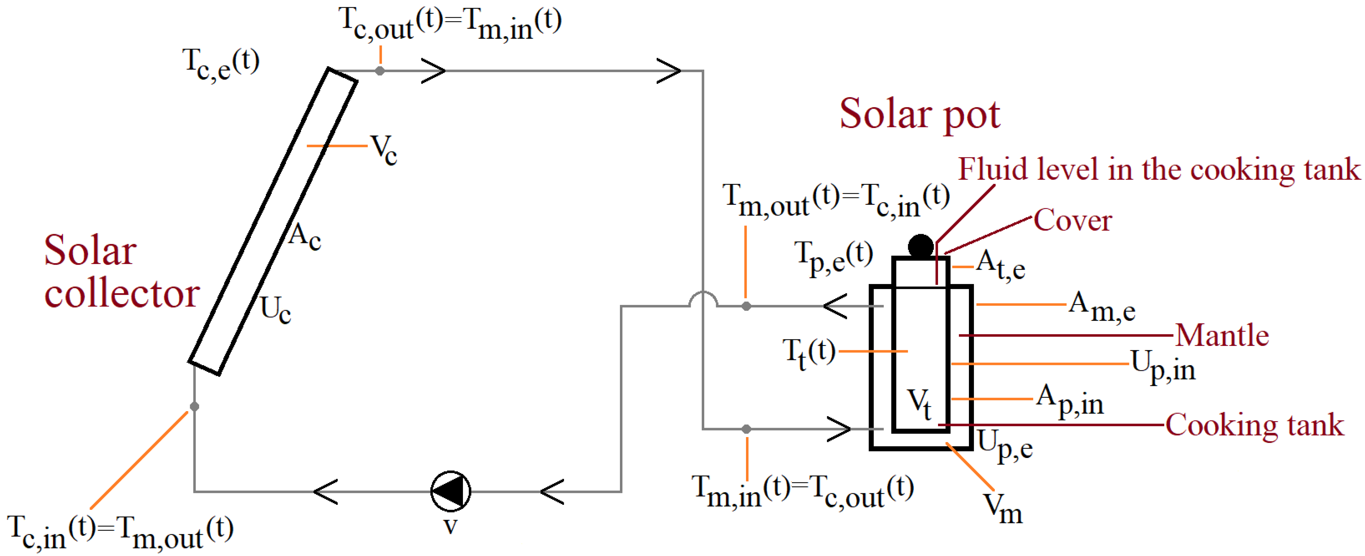
2. System Description

The solar pot (shown in Figure 1) is a recent invention, which gained a utility model protection in 2021 from the Hungarian Intellectual Property Office under patent number 5489 [33]. Currently, the pot is in prototype status, that is, a single specimen of it has been produced, from stainless steel (AISI 304) with a thickness of 2 mm, so far, for research purposes. However, it is already published by means of the mentioned patent, so it could be produced by a proper manufacturer commercially, in compliance with the related legal regulations.

The device is made for environmentally friendly cooking or heating of foods and liquids. Its structure is similar to a double pipe heat exchanger. It has an outer mantle and an inner cooking tank. Cooking or heating is done as follows. The mantle heats the cooking tank by circulating working medium (water or else) along the cooking tank’s outer surface. The mantle forms a closed hydraulic circuit with a solar collector. The working medium in the mantle and the interior of the cooking tank are hydraulically separated from each other, which implies heating and cooking can be executed hygienically. The pot can also be used for reheating foods or heating liquids not only in connection with food preparation. Using the device, heating and cooking can be made with the utilization of renewable solar energy. The solar pot has the advantage that it can be connected to an existing solar heating system. It is an indirect-type food processing equipment, which can be used with any collector using liquid as working fluid. If there is insufficient solar energy, one can heat the pot with a stove or a cooking plate as well.

In the experimental system of this paper, the solar pot is connected to an evacuated tube solar collector. Figure 2 presents the sketch of the pot containing the main geometric sizes and measuring points (for three temperatures) on it.

The experimental solar heating system with the solar pot and the time-dependent variables along with the parameters of the system are shown in Figure 3.

In Figure 3, t denotes the time dependence of the variables. These variables are the following:

• ${\mathrm{T}}_{\mathrm{c},\mathrm{e}}$: temperature of the solar collectors’s environment (outdoors), °C,
• ${\mathrm{T}}_{\mathrm{c},\mathrm{i}\mathrm{n}}$: solar collector inlet (water) temperature, °C,
• ${\mathrm{T}}_{\mathrm{c},\mathrm{o}\mathrm{u}\mathrm{t}}$: solar collector outlet (water) temperature, °C,
• ${\mathrm{T}}_{\mathrm{t}}$: temperature in the cooking tank, °C,
• ${\mathrm{T}}_{\mathrm{p},\mathrm{e}}$: temperature of the solar pot’s environment (indoors), °C,
• ${\mathrm{T}}_{\mathrm{m},\mathrm{i}\mathrm{n}}$: mantle inlet (water) temperature, °C,
• ${\mathrm{T}}_{\mathrm{m},\mathrm{o}\mathrm{u}\mathrm{t}}$: mantle outlet (water) temperature, °C.

As the fluid in the mantle is considered mixed, the (homogeneous) temperature inside the mantle is (consequently) considered the same as the mantle outlet temperature. (Basically, this temperature also corresponds to the, geometrically, mean fluid temperature in the mantle.) As the pipes connecting the solar pot and the collector are insulated and their volume is neglected, we consider the solar collector outlet temperature and the mantle inlet temperature equal $\left({\mathrm{T}}_{\mathrm{c},\mathrm{o}\mathrm{u}\mathrm{t}}={\mathrm{T}}_{\mathrm{m},\mathrm{i}\mathrm{n}}\right)$. The same holds for the solar collector inlet temperature and the mantle outlet temperature $\left({\mathrm{T}}_{\mathrm{c},\mathrm{i}\mathrm{n}}={\mathrm{T}}_{\mathrm{m},\mathrm{o}\mathrm{u}\mathrm{t}}\right)$.

The constant parameters of the system are the following:

• ${\mathrm{A}}_{\mathrm{c}}$: surface area of the collector (one side), ${\mathrm{m}}^2$,
• ${\mathrm{A}}_{\mathrm{m},\mathrm{e}}$: surface area of the mantle to the environment, ${\mathrm{m}}^2$,
• ${\mathrm{A}}_{\mathrm{t},\mathrm{e}}$: surface area of the cooking tank to the environment, ${\mathrm{m}}^2$,
• ${\mathrm{A}}_{\mathrm{p},\mathrm{i}\mathrm{n}}$: surface area between the mantle and the cooking tank, ${\mathrm{m}}^2$,
• ${\mathrm{U}}_{\mathrm{c}}$: overall heat loss coefficient of the solar collector, ${\displaystyle \frac{\mathrm{W}}{{\mathrm{m}}^2\mathrm{K}}}$,
• ${\mathrm{U}}_{\mathrm{p},\mathrm{e}}$: overall heat loss coefficient of the solar pot, ${\displaystyle \frac{\mathrm{W}}{{\mathrm{m}}^2\mathrm{K}}}$,
• ${\mathrm{U}}_{\mathrm{p},\mathrm{i}\mathrm{n}}$: overall heat transfer coefficient between the mantle and the cooking tank, ${\displaystyle \frac{\mathrm{W}}{{\mathrm{m}}^2\mathrm{K}}}$,
• v: volumetric flow rate of the pump, ${\displaystyle \frac{{\mathrm{m}}^3}{\mathrm{s}}}$,
• ${\mathrm{V}}_{\mathrm{c}}$: volume of the collector, ${\mathrm{m}}^3$,
• ${\mathrm{V}}_{\mathrm{m}}$: volume of the mantle, ${\mathrm{m}}^3$,
• ${\mathrm{V}}_{\mathrm{t}}$: volume of the cooking tank, ${\mathrm{m}}^3$.

During the tests, the cooking tank is filled with water up to the top of the mantle and covered by a stainless steel plate. The stainless steel cover can be removed during the cooking process to check the state of the handled food or drink. Accordingly, there is atmospheric pressure inside the cooking tank. We also circulate water between the solar pot and the solar collector as the working fluid.

3. Mathematical Modelling

The model of the solar pot is a physically-based mathematical model based on the energy balance of the pot. It consists of two submodels (due to the jacketed structure of the pot), one for the mantle temperature and the other for the cooking tank temperature, constituting a system of differential equations. Both equations are non-homogeneous linear differential equations with constant coefficients. The model uses temperature differences only, which allows the use of either Celsius or Kelvin values.

3.1. Mathematical Model

Equations (1) and (2) represent the model of the solar pot. Equation (1) is for the mantle, while Equation (2) is for the cooking tank temperature:

$${\displaystyle \frac{\mathrm{d}{\mathrm{T}}_{\mathrm{m},\mathrm{o}\mathrm{u}\mathrm{t}}}{\mathrm{d}\mathrm{t}}}={\displaystyle \frac{\mathrm{v}}{{\mathrm{V}}_{\mathrm{m}}}}\left({\mathrm{T}}_{\mathrm{m},\mathrm{i}\mathrm{n}}-{\mathrm{T}}_{\mathrm{m},\mathrm{o}\mathrm{u}\mathrm{t}}\right)+{\displaystyle \frac{{\mathrm{A}}_{\mathrm{m},\mathrm{e}}{\mathrm{U}}_{\mathrm{p},\mathrm{e}}}{\mathsf{\rho }\mathrm{c}{\mathrm{V}}_{\mathrm{m}}}}\left({\mathrm{T}}_{\mathrm{p},\mathrm{e}}-{\mathrm{T}}_{\mathrm{m},\mathrm{o}\mathrm{u}\mathrm{t}}\right)+{\displaystyle \frac{{\mathrm{A}}_{\mathrm{p},\mathrm{i}\mathrm{n}}{\mathrm{U}}_{\mathrm{p},\mathrm{i}\mathrm{n}}}{\mathsf{\rho }\mathrm{c}{\mathrm{V}}_{\mathrm{m}}}}\left({\mathrm{T}}_{\mathrm{t}}-{\mathrm{T}}_{\mathrm{m},\mathrm{o}\mathrm{u}\mathrm{t}}\right),$$

(1)

$${\displaystyle \frac{\mathrm{d}{\mathrm{T}}_{\mathrm{t}}}{\mathrm{d}\mathrm{t}}}={\displaystyle \frac{{\mathrm{A}}_{\mathrm{p},\mathrm{i}\mathrm{n}}{\mathrm{U}}_{\mathrm{p},\mathrm{i}\mathrm{n}}}{\mathsf{\rho }\mathrm{c}{\mathrm{V}}_{\mathrm{t}}}}\left({\mathrm{T}}_{\mathrm{m},\mathrm{o}\mathrm{u}\mathrm{t}}-{\mathrm{T}}_{\mathrm{t}}\right)+{\displaystyle \frac{{\mathrm{A}}_{\mathrm{t},\mathrm{e}}{\mathrm{U}}_{\mathrm{p},\mathrm{e}}}{\mathsf{\rho }\mathrm{c}{\mathrm{V}}_{\mathrm{t}}}}\left({\mathrm{T}}_{\mathrm{p},\mathrm{e}}-{\mathrm{T}}_{\mathrm{t}}\right),$$

(2)

where the density of water is $\mathsf{\rho }$ and the specific heat capacity is c.

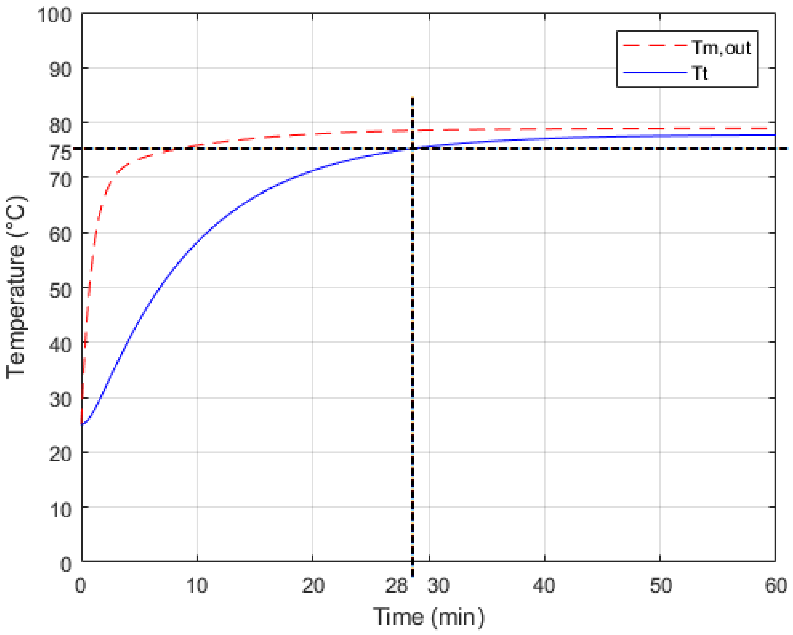
3.2. Simulation Results

Equations (1) and (2) were fed into the Matlab/Simulink programming environment. The computer realization of the model can be seen in Figure 4.

To run the model, the values of the solar pot’s parameters need to be provided. ${\mathrm{A}}_{\mathrm{m},\mathrm{e}}=0.19 {\mathrm{m}}^2$, ${\mathrm{A}}_{\mathrm{t},\mathrm{e}}=0.041 {\mathrm{m}}^2$, ${\mathrm{A}}_{\mathrm{p},\mathrm{i}\mathrm{n}}=0.112 {\mathrm{m}}^2$, ${\mathrm{V}}_{\mathrm{m}}=3.691 \mathrm{L}(=3.691·{10}^{-3} {\mathrm{m}}^3)$, and ${\mathrm{V}}_{\mathrm{t}}=4.418 \mathrm{L}(=4.418·{10}^{-3} {\mathrm{m}}^3)$ are geometric parameters of the physically manufactured solar pot (see Figure 1 in Section 2). The density ($\mathsf{\rho }$) and specific heat capacity (c) of water are also needed. These values are $1000 {\displaystyle \frac{\mathrm{k}\mathrm{g}}{{\mathrm{m}}^3}}$ and $4200 {\displaystyle \frac{\mathrm{J}}{\mathrm{k}\mathrm{g}\mathrm{K}}}$, respectively.

The determinations of ${\mathrm{U}}_{\mathrm{p},\mathrm{e}}=20.4 {\displaystyle \frac{\mathrm{W}}{{\mathrm{m}}^2\mathrm{K}}}$ (overall heat loss coefficient) and ${\mathrm{U}}_{\mathrm{p},\mathrm{i}\mathrm{n}}=351 {\displaystyle \frac{\mathrm{W}}{{\mathrm{m}}^2\mathrm{K}}}$ (overall heat transfer coefficient) are made by calculations based on recommendations from the literature.

${\mathrm{U}}_{\mathrm{p},\mathrm{e}}$ is the overall heat loss coefficient between the mantle and the solar pot’s environment. It is determined by considering the following:

• Convective heat transfer between the inside of the mantle and the inner surface of the mantle’s wall. (This wall is adjacent to the environment.) Taking into account the liquid in the mantle (water) and the material of the mantle’s wall (stainless steel), and assuming forced convective heat transfer along the inner surface of the mantle’s wall, the heat transfer coefficient is $850 {\displaystyle \frac{\mathrm{W}}{{\mathrm{m}}^2\mathrm{K}}}$, which is an average value according to [34].
• Thermal conduction inside the mantle’s wall. Taking into account the material of the mantle’s wall, which is stainless steel (with a thickness of 0.002 m), the thermal conductivity coefficient is $15 {\displaystyle \frac{\mathrm{W}}{\mathrm{m}\mathrm{K}}}$, which is an average value according to [34].
• Convective heat transfer between the outer surface of the mantle’s wall and the solar pot’s environment. Taking into account the material of the mantle’s wall (stainless steel) and the air surrounding the pot from outside, and assuming free convective heat transfer along the surface of the wall, the heat transfer coefficient is $21 {\displaystyle \frac{\mathrm{W}}{{\mathrm{m}}^2\mathrm{K}}}$, which is an average value according to [34].

The above details were fed into the [35] online program, which made the necessary calculations for the overall heat loss coefficient. The result is ${\mathrm{U}}_{\mathrm{p},\mathrm{e}}=20.4 {\displaystyle \frac{\mathrm{W}}{{\mathrm{m}}^2\mathrm{K}}}$.

In the value of ${\mathrm{A}}_{\mathrm{t},\mathrm{e}}$ (which is the responsible surface regarding the heat loss of the cooking tank to the environment), the surface area of both the cover and that part of the tank’s wall which is above the mantle are included. Furthermore, ${\mathrm{U}}_{\mathrm{p},\mathrm{e}}$ is applied to this surface when determining the heat loss of the cooking tank to the environment. Of course, this approach contains certain simplifications (which is clearly advantageous when one would like to apply the model in the practice) since it does not take into account that there is some air between the tank’s fluid and the cover. Nevertheless, it must underestimate the pot’s real heat performance a bit since the air has some (advantageous) thermal insulating effect. It also means that we do not provide even a slight advantage for the solar pot when presenting its potential applicability. In addition, we carried out simulations (not detailed here) where we tried to model the special effect of the air under the cover. In fact, the difference was so slight (within 1% regarding the modelled temperature values) that we think they are not worth dealing with in the present model.

${\mathrm{U}}_{\mathrm{p},\mathrm{i}\mathrm{n}}$ is the overall heat transfer coefficient between the mantle and the cooking tank. It is determined by considering the following:

• Convective heat transfer between the inside of the mantle and the outer surface of the cooking tank’s wall. Taking into account the liquid in the mantle (water) and the material of the cooking tank wall (stainless steel), and assuming forced convective heat transfer along the surface of the wall, the heat transfer coefficient is $850 {\displaystyle \frac{\mathrm{W}}{{\mathrm{m}}^2\mathrm{K}}}$, which is an average value according to [34].
• Thermal conduction inside the mantle’s wall. (For more details, see Note 2 above.)
• Convective heat transfer between the inner surface of the cooking tank’s wall and the inside of the cooking tank. Taking into account the material of the wall (stainless steel) and the liquid in the cooking tank (water), and assuming free convective heat transfer along the surface of the wall, the heat transfer coefficient is $650 {\displaystyle \frac{\mathrm{W}}{{\mathrm{m}}^2\mathrm{K}}}$, which is an average value according to [34].

The above details were fed into the [35] online program, which made the necessary calculations for the overall heat transfer coefficient. The result is ${\mathrm{U}}_{\mathrm{p},\mathrm{i}\mathrm{n}}=351 {\displaystyle \frac{\mathrm{W}}{{\mathrm{m}}^2\mathrm{K}}}$.

${\mathrm{T}}_{\mathrm{p},\mathrm{e}}\left(\mathrm{t}\right)$ is assumed to be constant as the solar pot is located in an air-conditioned mobile container, so ${{\mathrm{T}}_{\mathrm{p},\mathrm{e}}:\mathrm{T}}_{\mathrm{p},\mathrm{e}}\left(\mathrm{t}\right):25 °\mathrm{C}$, in accordance with the temperature set inside the container. The initial values of the model are also set to this value, so ${\mathrm{T}}_{\mathrm{m},\mathrm{o}\mathrm{u}\mathrm{t}}\left(0\right):25 °\mathrm{C}$ and ${\mathrm{T}}_{\mathrm{t}}\left(0\right):25 °\mathrm{C}$. (Accordingly, our model can be applied for a solar pot inside a building, which is a rather general situation, since the outside effects, like the effect of sky, solar irradiance, wind speed etc. are not considered.) For the sake of simplicity, ${\mathrm{T}}_{\mathrm{m},\mathrm{i}\mathrm{n}}\left(\mathrm{t}\right){(=\mathrm{T}}_{\mathrm{c},\mathrm{o}\mathrm{u}\mathrm{t}}\left(\mathrm{t}\right))$ is set constant in the simulations, 80 °C. Choosing this temperature value, it was taken into consideration that it can easily be reached and maintained for a longer time on a typical day in May in Hungary and that this inlet temperature is probably high enough for the cooking tank to reach the minimum temperature for sterilizing foods—based on our preliminary assumption. This minimum temperature is 73.9 °C, but in this work 75 °C is aimed due to safety purposes. The simulations were carried out with two different volumetric flow rate ($\mathrm{v}$) values, which can be realized in the experimental system as well. The results of the simulations are presented in Figure 5 and Figure 6. More specifically, Figure 5 presents the modelled ${\mathrm{T}}_{\mathrm{m},\mathrm{o}\mathrm{u}\mathrm{t}}$ and ${\mathrm{T}}_{\mathrm{t}}$ temperatures in case of $\mathrm{v}=100 {\displaystyle \frac{\mathrm{L}}{\mathrm{h}}}(=2.78·{10}^{-5} {\displaystyle \frac{{\mathrm{m}}^3}{s}})$, while Figure 6 presents them in case of $\mathrm{v}=200 {\displaystyle \frac{\mathrm{L}}{\mathrm{h}}}(=5.56·{10}^{-5} {\displaystyle \frac{{\mathrm{m}}^3}{s}})$. The running time of the simulations was 1 h in both cases.

In Figure 5 and Figure 6, it can be seen that the cooking tank temperature reaches 75 °C, which is normally enough for the sterilization of foods. It can also be stated that this temperature is reached in less time with higher flow rate. With $100 {\displaystyle \frac{\mathrm{L}}{\mathrm{h}}}$, it took 38 min (see Figure 5), while with $200 {\displaystyle \frac{\mathrm{L}}{\mathrm{h}}}$, it required 28 min (see Figure 6). In addition, the maximum (final) tank temperature was 76.5 °C in case of $100 {\displaystyle \frac{\mathrm{L}}{\mathrm{h}}}$ and 77.7 °C with $200 {\displaystyle \frac{\mathrm{L}}{\mathrm{h}}}$.

3.3. Exact Calculation of the Equilibrium

Equations (3) and (4) represent the determining formulas for the equilibrium values of the modelled temperatures (${\mathrm{T}}_{\mathrm{m},\mathrm{o}\mathrm{u}\mathrm{t}}$ and ${\mathrm{T}}_{\mathrm{t}}$) in accordance with that the derivatives (at the left hand side of Equations (1) and (2) should be zero in the equilibrium. The equilibrium values of ${\mathrm{T}}_{\mathrm{m},\mathrm{o}\mathrm{u}\mathrm{t}}$ and ${\mathrm{T}}_{\mathrm{t}}$ are denoted by ${\mathrm{T}}_{\mathrm{m},\mathrm{o}\mathrm{u}\mathrm{t},\mathrm{e}\mathrm{q}}$ and ${\mathrm{T}}_{\mathrm{t},\mathrm{e}\mathrm{q}}$, respectively.

$$0={\displaystyle \frac{\mathrm{v}}{{\mathrm{V}}_{\mathrm{m}}}}\left({\mathrm{T}}_{\mathrm{m},\mathrm{i}\mathrm{n}}-{\mathrm{T}}_{\mathrm{m},\mathrm{o}\mathrm{u}\mathrm{t},\mathrm{e}\mathrm{q}}\right)+{\displaystyle \frac{{\mathrm{A}}_{\mathrm{m},\mathrm{e}}{\mathrm{U}}_{\mathrm{p},\mathrm{e}}}{\mathsf{\rho }\mathrm{c}{\mathrm{V}}_{\mathrm{m}}}}\left({\mathrm{T}}_{\mathrm{p},\mathrm{e}}-{\mathrm{T}}_{\mathrm{m},\mathrm{o}\mathrm{u}\mathrm{t},\mathrm{e}\mathrm{q}}\right)+{\displaystyle \frac{{\mathrm{A}}_{\mathrm{p},\mathrm{i}\mathrm{n}}{\mathrm{U}}_{\mathrm{p},\mathrm{i}\mathrm{n}}}{\mathsf{\rho }\mathrm{c}{\mathrm{V}}_{\mathrm{m}}}}\left({\mathrm{T}}_{\mathrm{t},\mathrm{e}\mathrm{q}}-{\mathrm{T}}_{\mathrm{m},\mathrm{o}\mathrm{u}\mathrm{t},\mathrm{e}\mathrm{q}}\right),$$

(3)

$$0={\displaystyle \frac{{\mathrm{A}}_{\mathrm{p},\mathrm{i}\mathrm{n}}{\mathrm{U}}_{\mathrm{p},\mathrm{i}\mathrm{n}}}{\mathsf{\rho }\mathrm{c}{\mathrm{V}}_{\mathrm{t}}}}\left({\mathrm{T}}_{\mathrm{m},\mathrm{o}\mathrm{u}\mathrm{t},\mathrm{e}\mathrm{q}}-{\mathrm{T}}_{\mathrm{t},\mathrm{e}\mathrm{q}}\right)+{\displaystyle \frac{{\mathrm{A}}_{\mathrm{t},\mathrm{e}}{\mathrm{U}}_{\mathrm{p},\mathrm{e}}}{\mathsf{\rho }\mathrm{c}{\mathrm{V}}_{\mathrm{t}}}}\left({\mathrm{T}}_{\mathrm{p},\mathrm{e}}-{\mathrm{T}}_{\mathrm{t},\mathrm{e}\mathrm{q}}\right),$$

(4)

from which the equilibrium temperatures can be expressed explicitly as follows:

$$\begin{array}{l}{\mathrm{T}}_{\mathrm{m},\mathrm{o}\mathrm{u}\mathrm{t},\mathrm{e}\mathrm{q}}\\ ={\displaystyle \frac{{\mathrm{A}}_{\mathrm{p},\mathrm{i}\mathrm{n}}{\mathrm{U}}_{\mathrm{p},\mathrm{i}\mathrm{n}}\mathrm{v}\mathsf{\rho }\mathrm{c}{\mathrm{T}}_{\mathrm{m},\mathrm{i}\mathrm{n}}+{\mathrm{A}}_{\mathrm{p},\mathrm{i}\mathrm{n}}{\mathrm{U}}_{\mathrm{p},\mathrm{i}\mathrm{n}}{\mathrm{A}}_{\mathrm{m},\mathrm{e}}{\mathrm{U}}_{\mathrm{p},\mathrm{e}}{\mathrm{T}}_{\mathrm{p},\mathrm{e}}+{\mathrm{A}}_{\mathrm{m},\mathrm{e}}{U}_{p,e}^2{\mathrm{A}}_{\mathrm{t},\mathrm{e}}{\mathrm{T}}_{\mathrm{p},\mathrm{e}}+{\mathrm{A}}_{\mathrm{p},\mathrm{i}\mathrm{n}}{\mathrm{U}}_{\mathrm{p},\mathrm{i}\mathrm{n}}{\mathrm{A}}_{\mathrm{t},\mathrm{e}}{{\mathrm{U}}_{\mathrm{p},\mathrm{e}}\mathrm{T}}_{\mathrm{p},\mathrm{e}}+{\mathrm{A}}_{\mathrm{t},\mathrm{e}}{\mathrm{U}}_{\mathrm{p},\mathrm{e}}\mathrm{v}\mathsf{\rho }\mathrm{c}{\mathrm{T}}_{\mathrm{m},\mathrm{i}\mathrm{n}}}{{\mathrm{A}}_{\mathrm{p},\mathrm{i}\mathrm{n}}{\mathrm{U}}_{\mathrm{p},\mathrm{i}\mathrm{n}}\mathrm{v}\mathsf{\rho }\mathrm{c}+{\mathrm{A}}_{\mathrm{t},\mathrm{e}}{\mathrm{U}}_{\mathrm{p},\mathrm{e}}\mathrm{v}\mathsf{\rho }\mathrm{c}+{\mathrm{A}}_{\mathrm{p},\mathrm{i}\mathrm{n}}{\mathrm{U}}_{\mathrm{p},\mathrm{i}\mathrm{n}}{\mathrm{A}}_{\mathrm{m},\mathrm{e}}{\mathrm{U}}_{\mathrm{p},\mathrm{e}}+{\mathrm{A}}_{\mathrm{m},\mathrm{e}}{U}_{p,e}^2{\mathrm{A}}_{\mathrm{t},\mathrm{e}}+{\mathrm{A}}_{\mathrm{p},\mathrm{i}\mathrm{n}}{\mathrm{U}}_{\mathrm{p},\mathrm{i}\mathrm{n}}{\mathrm{A}}_{\mathrm{t},\mathrm{e}}{\mathrm{U}}_{\mathrm{p},\mathrm{e}}}},\end{array}$$

(5)

$${\mathrm{T}}_{\mathrm{t},\mathrm{e}\mathrm{q}}={\displaystyle \frac{{\mathrm{A}}_{\mathrm{p},\mathrm{i}\mathrm{n}}{\mathrm{U}}_{\mathrm{p},\mathrm{i}\mathrm{n}}\mathrm{v}\mathsf{\rho }\mathrm{c}{\mathrm{T}}_{\mathrm{m},\mathrm{i}\mathrm{n}}+{\mathrm{A}}_{\mathrm{p},\mathrm{i}\mathrm{n}}{\mathrm{U}}_{\mathrm{p},\mathrm{i}\mathrm{n}}{\mathrm{A}}_{\mathrm{m},\mathrm{e}}{\mathrm{U}}_{\mathrm{p},\mathrm{e}}{\mathrm{T}}_{\mathrm{p},\mathrm{e}}+{\mathrm{A}}_{\mathrm{m},\mathrm{e}}{U}_{p,e}^2{\mathrm{A}}_{\mathrm{t},\mathrm{e}}{\mathrm{T}}_{\mathrm{p},\mathrm{e}}+{\mathrm{A}}_{\mathrm{p},\mathrm{i}\mathrm{n}}{\mathrm{U}}_{\mathrm{p},\mathrm{i}\mathrm{n}}{\mathrm{A}}_{\mathrm{t},\mathrm{e}}{{\mathrm{U}}_{\mathrm{p},\mathrm{e}}\mathrm{T}}_{\mathrm{p},\mathrm{e}}+{\mathrm{A}}_{\mathrm{t},\mathrm{e}}{\mathrm{U}}_{\mathrm{p},\mathrm{e}}\mathrm{v}\mathsf{\rho }\mathrm{c}{\mathrm{T}}_{\mathrm{p},\mathrm{e}}}{{\mathrm{A}}_{\mathrm{p},\mathrm{i}\mathrm{n}}{\mathrm{U}}_{\mathrm{p},\mathrm{i}\mathrm{n}}\mathrm{v}\mathsf{\rho }\mathrm{c}+{\mathrm{A}}_{\mathrm{t},\mathrm{e}}{\mathrm{U}}_{\mathrm{p},\mathrm{e}}\mathrm{v}\mathsf{\rho }\mathrm{c}+{\mathrm{A}}_{\mathrm{p},\mathrm{i}\mathrm{n}}{\mathrm{U}}_{\mathrm{p},\mathrm{i}\mathrm{n}}{\mathrm{A}}_{\mathrm{m},\mathrm{e}}{\mathrm{U}}_{\mathrm{p},\mathrm{e}}+{\mathrm{A}}_{\mathrm{m},\mathrm{e}}{U}_{p,e}^2{\mathrm{A}}_{\mathrm{t},\mathrm{e}}+{\mathrm{A}}_{\mathrm{p},\mathrm{i}\mathrm{n}}{\mathrm{U}}_{\mathrm{p},\mathrm{i}\mathrm{n}}{\mathrm{A}}_{\mathrm{t},\mathrm{e}}{\mathrm{U}}_{\mathrm{p},\mathrm{e}}}}.$$

(6)

After substituting the above parameter values (${\mathrm{A}}_{\mathrm{m},\mathrm{e}}=0.19{\mathrm{m}}^2$, ${\mathrm{A}}_{\mathrm{t},\mathrm{e}}=0.041{\mathrm{m}}^2$, …) into Equations (5) and (6), 77.9 °C and 78.9 °C is resulted in case of $100 {\displaystyle \frac{\mathrm{L}}{\mathrm{h}}}$ and $200 {\displaystyle \frac{\mathrm{L}}{\mathrm{h}}}$, respectively, for ${\mathrm{T}}_{\mathrm{m},\mathrm{o}\mathrm{u}\mathrm{t},\mathrm{e}\mathrm{q}}$, and 76.8 °C and 77.8 °C is resulted in case of $100 {\displaystyle \frac{\mathrm{L}}{\mathrm{h}}}$ and $200 {\displaystyle \frac{\mathrm{L}}{\mathrm{h}}}$, respectively, for ${\mathrm{T}}_{\mathrm{t},\mathrm{e}\mathrm{q}}$. Taking into account that the simulated final tank temperature was 76.5 °C and 77.7 °C in case of $100 {\displaystyle \frac{\mathrm{L}}{\mathrm{h}}}$ and $200 {\displaystyle \frac{\mathrm{L}}{\mathrm{h}}}$, respectively, at the end of Section 3.2, we can state that the (estimated) numerical (simulated) temperature values are well in accordance with the exact equilibrium values. (It is normal that the monotonically increasing simulated values are slightly lower since the equilibrium could be reached in infinitely long time, in principle.) Considering that the initial temperature values in the simulations (25 °C) was rather far from the exact equilibrium values, it is suggested that the equilibrium is (globally asymptotically) stable.

4. Experimentation

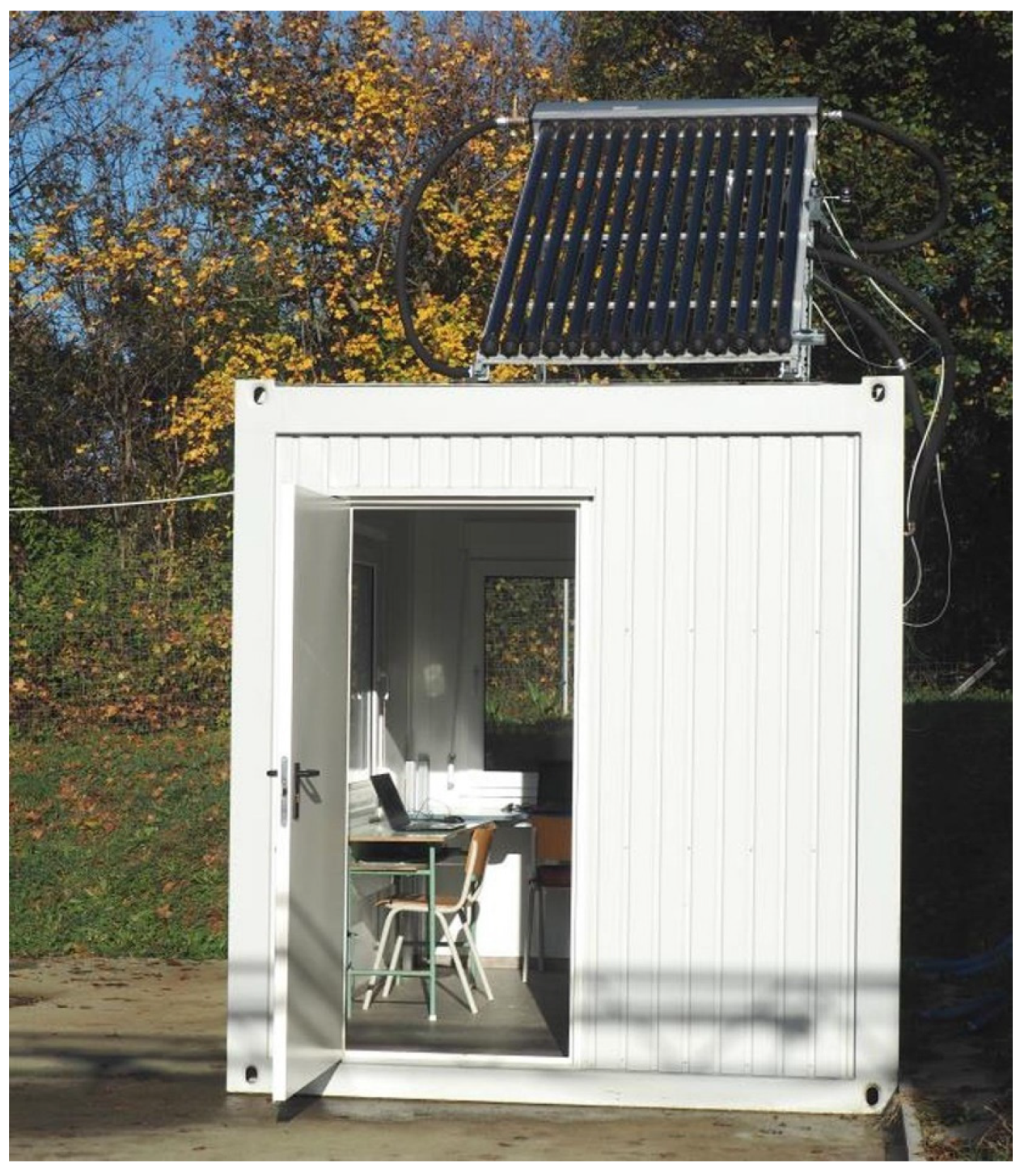
4.1. Experimental System

During the measurements, the values of ${\mathrm{T}}_{\mathrm{c},\mathrm{e}}$, ${\mathrm{T}}_{\mathrm{m},\mathrm{i}\mathrm{n}} (={\mathrm{T}}_{\mathrm{c},\mathrm{o}\mathrm{u}\mathrm{t}})$, ${\mathrm{T}}_{\mathrm{m},\mathrm{o}\mathrm{u}\mathrm{t}} (={\mathrm{T}}_{\mathrm{c},\mathrm{i}\mathrm{n}})$, ${\mathrm{T}}_{\mathrm{p},\mathrm{e}}$, ${\mathrm{T}}_{\mathrm{t}}$ and $\mathrm{v}$ are measured. The temperatures are measured with K-type thermocouples (with an average uncertainty of 1 °C), the pump flow rate is measured with a Kobold Unirota URM-33 33H G5 (Nyíregyháza, Hungary) 0 type flow meter (with an average uncertainty of $6 {\displaystyle \frac{\mathrm{L}}{\mathrm{h}}}$). As additional information, the (global) solar irradiance on the collector’s plane is also measured (in ${\displaystyle \frac{\mathrm{W}}{{\mathrm{m}}^2}}$). The type of the solar irradiance sensor is Theodor Friedrichs 6003.3000 BG (Elmshorn, Germany) (with an average uncertainty of $30 {\displaystyle \frac{\mathrm{W}}{{\mathrm{m}}^2}}$). The collector, with $2.2 {\mathrm{m}}^2$, is oriented to the south, its tilt angle is 40°.

The pipes connecting the solar pot and the collector are insulated and their volume is neglected. As a result, we consider the mantle inlet water temperature and the solar collector outlet water temperature equal $\left({\mathrm{T}}_{\mathrm{m},\mathrm{i}\mathrm{n}}={\mathrm{T}}_{\mathrm{c},\mathrm{o}\mathrm{u}\mathrm{t}}\right)$. The same goes for the mantle outlet water temperature and the solar collector inlet water temperature $\left({\mathrm{T}}_{\mathrm{m},\mathrm{o}\mathrm{u}\mathrm{t}}={\mathrm{T}}_{\mathrm{c},\mathrm{i}\mathrm{n}}\right)$. The structure of the experimental system, installed at the campus of the Hungarian University of Agriculture and Life Sciences (Gödöllő, Hungary), is shown in Figure 3, the physically manufactured solar pot is presented in Figure 1 and the connected evacuated tube solar collector can be seen in Figure 7.

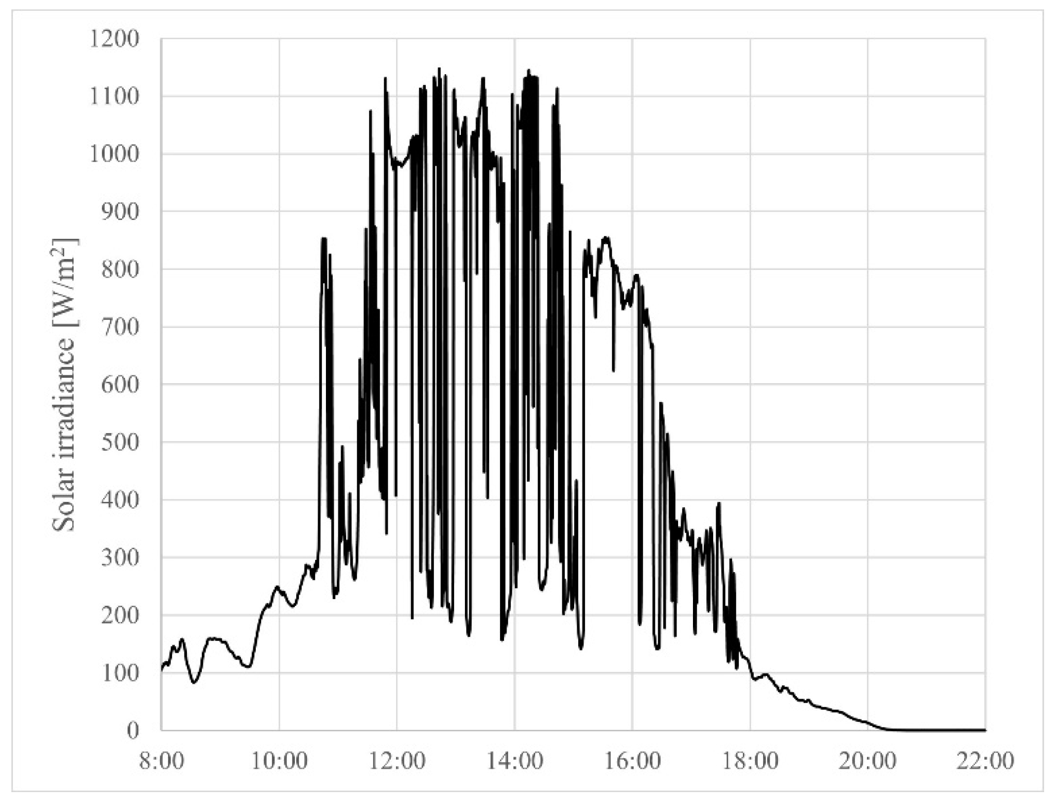
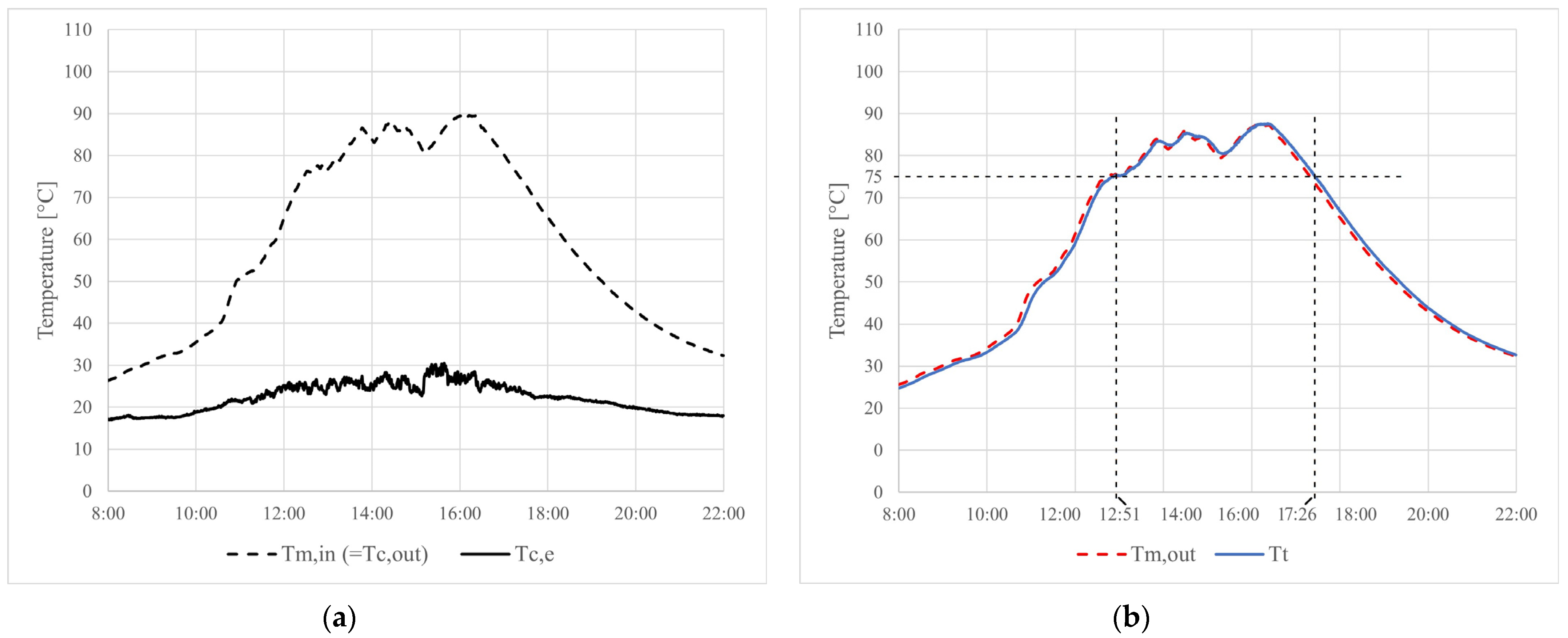
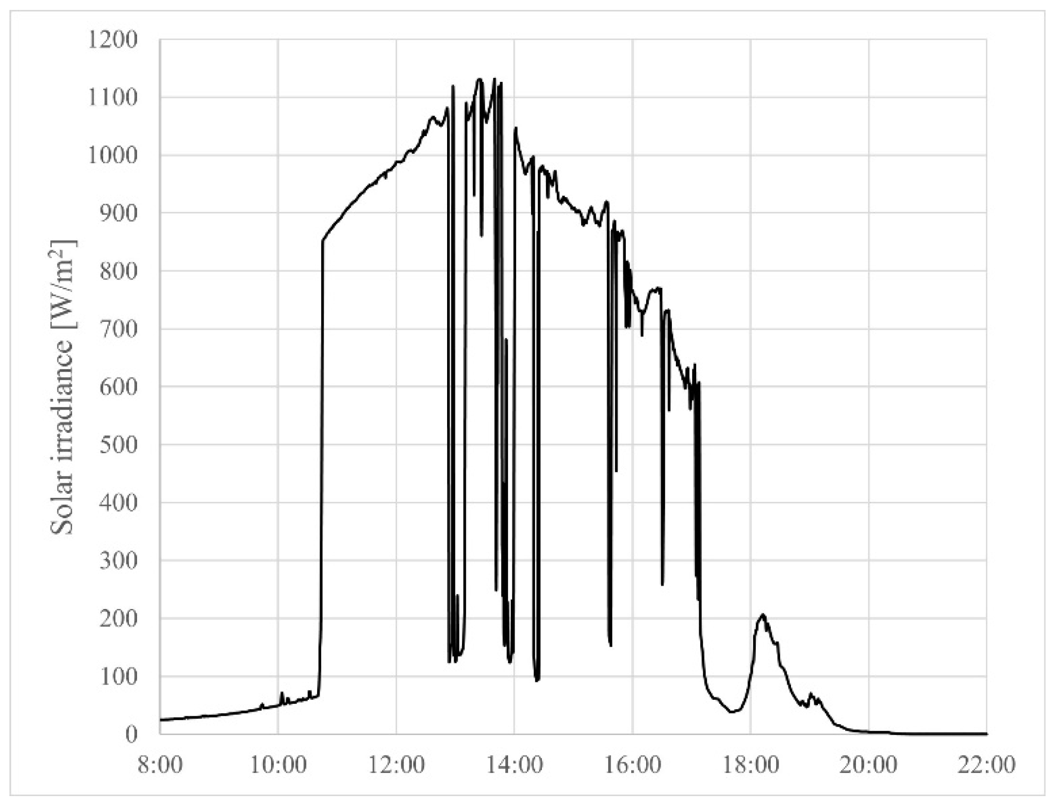
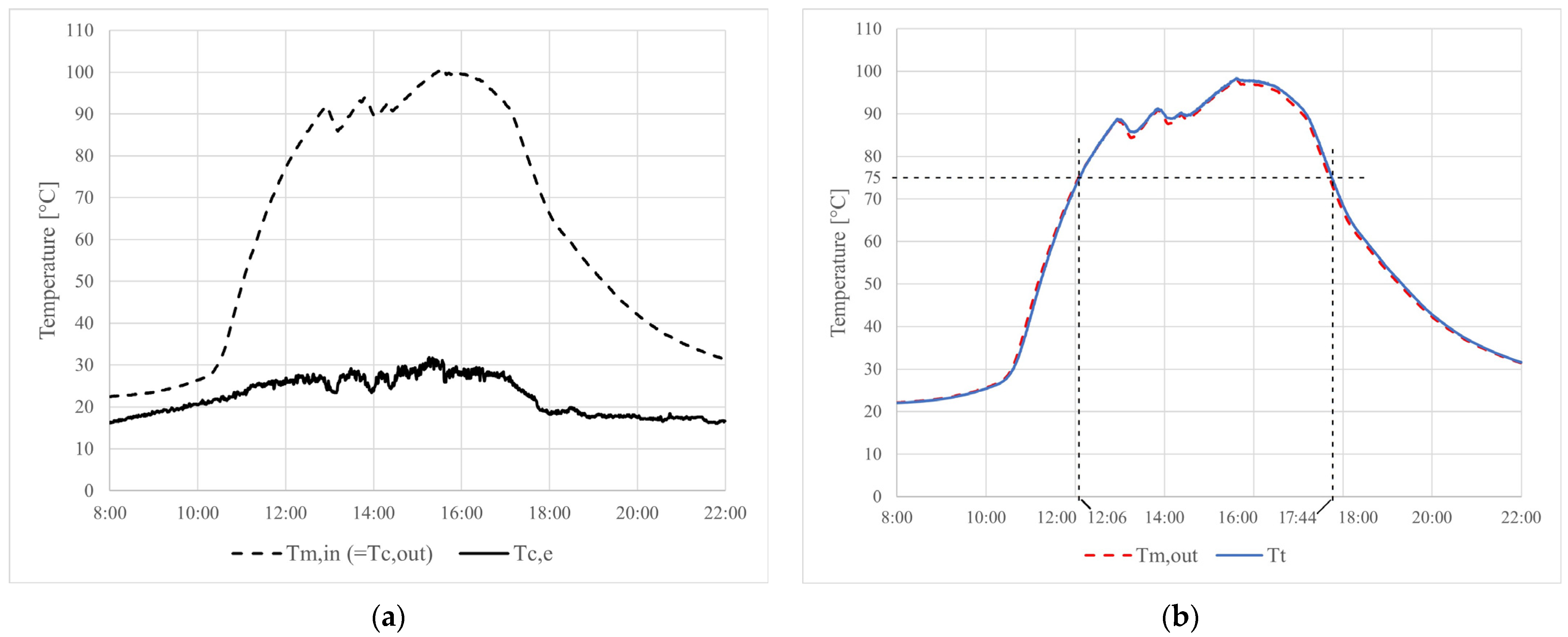
4.2. Experimental Results

During the measurements, the same flow rates were used as in the simulations. The temperature of the solar pot’s environment (${\mathrm{T}}_{\mathrm{p},\mathrm{e}}$) was also constant 25 °C as the temperature of the mobile container where the solar pot is located was set to this value with an air-conditioner. Figure 8, Figure 9, Figure 10, Figure 11, Figure 12, Figure 13, Figure 14 and Figure 15 present the graphs of all measurement results. Figure 9 and Figure 11 show the measurement results of two days (26 May 2024 and 28 May 2024) when the flow rate was set to $100 {\displaystyle \frac{\mathrm{L}}{\mathrm{h}}}$. In Figure 13 and Figure 15, the measured data of two days (29 and 30 May 2024) are presented when the flow rate was set to $200 {\displaystyle \frac{\mathrm{L}}{\mathrm{h}}}$. On the left side of the figures (a), the graphs of ${\mathrm{T}}_{\mathrm{m},\mathrm{i}\mathrm{n}} (={\mathrm{T}}_{\mathrm{c},\mathrm{o}\mathrm{u}\mathrm{t}})$ and ${\mathrm{T}}_{\mathrm{c},\mathrm{e}}$ can be seen, on the right (b), there are the graphs of ${\mathrm{T}}_{\mathrm{m},\mathrm{o}\mathrm{u}\mathrm{t}}$ and ${\mathrm{T}}_{\mathrm{t}}$. As additional information, Figure 8, Figure 10, Figure 12 and Figure 14 show the solar irradiance on the four measured days.

Figure 9, Figure 11, Figure 13 and Figure 15 demonstrate that the cooking tank temperature reached the safe cooking temperature of 75 °C during the measurements in the early afternoon, between 12:00 and 13:00. The temperature of the cooking tank was higher than this value until late afternoon, between 17:20 and 18:00. The only exception was on 30 May when the tank temperature decreased below 75 °C at 16:18 due to the cloudier weather than usual. According to the measurements, it can be stated that the volumetric flow rate has no considerable influence on the heating. Both examined flow rate values made the safe cooking possible for a satisfactory time interval within each measured day. The measured values of ${\mathrm{T}}_{\mathrm{m},\mathrm{o}\mathrm{u}\mathrm{t}}$ and ${\mathrm{T}}_{\mathrm{t}}$ are almost equal, which is in accordance with the final modelled temperature values in the simulations (see Figure 5 and Figure 6).

In summary, the measured results reinforce the simulated ones, which underlie that the solar pot is really able to cook (sterilize) safely (liquid) foods and drinks.

5. Conclusions

In the paper, a new physically-based mathematical model was proposed and an experimental system was assembled for a recently invented solar pot. The solar pot, as an environmentally friendly technical tool, utilizes renewable solar heat, provided by a solar collector as the heat source, for cooking or heating foods, drinks or other liquids. Based on both the simulated and the measured results, the solar pot, containing an inner cooking tank (where the cooking or heating task is realized) and an outer mantle (connected directly to the solar collector), can be used successfully to cook or sterilize different dishes and liquids. In particular, based on measured data, the temperature level needed for heat treatment (75 °C) can be maintained in the cooking tank for several hours (~5 h, on the average) in a typical day in May in Hungary.

Future research plans include the investigation of how long does it take for the solar pot-collector system to cook different dishes (like pasta, meat etc.) in different seasons and weather conditions. The possibility and relevance of different types of auxiliary (not solar) heating solutions (in addition to the solar collector) may also be examined, in order to extend the operating period of the solar pot. With respect to the proposed mathematical model, the establishment of a maximally precise version of it (considering sky effects, the effect of air under the cover, the temperature dependence of certain parameters, like the mass density and the specific heat capacity of water, etc.) may come into question in the future.

References

1. Kalita, N.; Muthukumar, P.; Dalal, A. Performance investigation of a hybrid solar dryer with electric and biogas backup air heaters for chilli drying. Therm. Sci. Eng. Prog. 2024, 52, 102646. [Google Scholar] [CrossRef]
2. Mehling, H. Use of phase change materials for food applications—State of the art in 2022. Appl. Sci. 2023, 13, 3354. [Google Scholar] [CrossRef]
3. Saxena, A.; Cuce, E.; Tiwari, G.N.; Kumar, A. Design and thermal performance investigation of a box cooker with flexible solar collector tubes: An experimental research. Energy 2020, 206, 118144. [Google Scholar] [CrossRef]
4. Bigelow, A.W.; Tabatchnick, J.; Hughes, C. Testing Solar Cookers for Cooking Efficiency. Sol. Energy Adv. 2024, 4, 100053. [Google Scholar] [CrossRef]
5. USDA (Food Safety and Inspection Service, U.S. Department of Agriculture). Safe Minimum Internal Temperature Chart. Available online: https://www.fsis.usda.gov/food-safety/safe-food-handling-and-preparation/food-safety-basics/safe-temperature-chart (accessed on 6 June 2024).
6. Gupta, P.K.; Misal, A.; Agrawal, S. Development of low cost reflective panel solar cooker. Mater. Today Proc. 2021, 45, 3010–3013. [Google Scholar] [CrossRef]
7. Saini, P.; Pandey, S.; Goswami, S.; Dhar, A.; Mohamed, M.E.; Powar, S. Experimental and numerical investigation of a hybrid solar thermal-electric powered cooking oven. Energy 2023, 280, 128188. [Google Scholar] [CrossRef]
8. Hosseinzadeh, M.; Faezian, A.; Mirzababaee, S.M. Parametric analysis and optimization of a portable evacuated tube solar cooker. Energy 2020, 194, 116816. [Google Scholar] [CrossRef]
9. Zhou, C.; Wang, Y.; Li, J.; Ma, X.; Li, Q.; Yang, M.; Zhao, X.; Zhu, Y. Simulation and economic analysis of an innovative indoor solar cooking system with energy storage. Sol. Energy 2023, 263, 111816. [Google Scholar] [CrossRef]
10. Hosseinzadeh, M.; Sadeghirad, R.; Zamani, H.; Kianifar, A.; Mirzababaee, S.M. The performance improvement of an indirect solar cooker using multi-walled carbon nanotube-oil nanofluid: An experimental study with thermodynamic analysis. Renew. Energy 2021, 165, 14–24. [Google Scholar] [CrossRef]
11. Hussein, H.M.S.; El-Ghetany, H.H.; Nada, S.A. Experimental investigation of novel indirect solar cooker with indoor PCM thermal storage and cooking unit. Energy Convers. Manag. 2008, 49, 2237–2246. [Google Scholar] [CrossRef]
12. Getnet, M.Y.; Gunjo, D.G.; Sinha, D.K. Experimental investigation of thermal storage integrated indirect solar cooker with and without reflectors. Results Eng. 2023, 18, 101022. [Google Scholar] [CrossRef]
13. Kumar, R.; Adhikari, R.S.; Garg, H.P.; Kumar, A. Thermal performance of a solar pressure cooker based on evacuated tube solar collector. Appl. Therm. Eng. 2001, 21, 1699–1706. [Google Scholar] [CrossRef]
14. Schwarzer, K.; Krings, T. Demonstrations-und Feldtest von Solarkochern mit Temporärem Speicher in Indien und Mali; Shaker Verlag: Aachen, Germany, 1996. (In German) [Google Scholar]
15. Buzás, J.; Farkas, I. Solar domestic hot water system simulation using blockoriented software. In The 3rd ISES-europe Solar World Congress; CD-ROM Proceedings: København, Denmark, 2000; pp. 1–9. [Google Scholar]
16. Castellanos, L.S.M.; Noguera, A.L.G.; Velásquez, E.I.G.; Caballero, G.E.C.; Lora, E.E.S.; Cobas, V.R.M. Mathematical modeling of a system composed of parabolic trough solar collectors integrated with a hydraulic energy storage system. Energy 2020, 208, 118255. [Google Scholar] [CrossRef]
17. Kalogirou, S.A.; Panteliou, S.; Dentsoras, A. Modeling of Solar Domestic Water Heating Systems Using Artificial Neural Networks. Sol. Energy 1999, 65, 335–342. [Google Scholar] [CrossRef]
18. Brus, L.; Zambrano, D. Black-box identification of solar collector dynamics with variant time delay. Control Eng. Pract. 2010, 18, 1133–1146. [Google Scholar] [CrossRef]
19. Zheng, J.; Febrer, R.; Castro, J.; Kizildag, D.; Rigola, J. A new high-performance flat plate solar collector. Numerical modelling and experimental validation. Appl. Energy 2023, 355, 122221. [Google Scholar] [CrossRef]
20. Hottel, H.C.; Woertz, B.B. The performance of flat plate solar heat collectors. Trans. ASME 1942, 64, 91–104. [Google Scholar] [CrossRef]
21. Buzás, J.; Farkas, I.; Biró, A.; Németh, R. Modelling and simulation aspects of a solar hot water system. Math. Comput. Simul. 1998, 48, 33–46. [Google Scholar] [CrossRef]
22. Hilmer, F.; Vajen, K.; Ratka, A.; Ackermann, H.; Fuhs, W.; Melsheimer, O. Numerical solution and validation of a dynamic model of solar collectors working with varying fluid flow rate. Sol. Energy 1999, 65, 305–321. [Google Scholar] [CrossRef]
23. Mao, C.; Li, M.; Li, N.; Shan, M.; Yang, X. Mathematical model development and optimal design of the horizontal all-glass evacuated tube solar collectors integrated with bottom mirror reflectors for solar energy harvesting. Appl. Energy 2019, 238, 54–68. [Google Scholar] [CrossRef]
24. Víg, P.G. Modelling of Solar Collector Systems with Neural Network. Ph.D. Thesis, Szent István University, Gödöllő, Hungary, 2007. (In Hungarian). [Google Scholar]
25. Kicsiny, R. Multiple linear regression based model for solar collectors. Sol. Energy 2014, 110, 496–506. [Google Scholar] [CrossRef]
26. Hiris, D.P.; Pop, O.G.; Balan, M.C. Analytical modeling and validation of the thermal behavior of seasonal storage tanks for solar district heating. Energy Rep. 2022, 8, 741–755. [Google Scholar] [CrossRef]
27. Badescu, V. Optimal control of flow in solar collector systems with fully mixed water storage tanks. Energy Convers. Manag. 2008, 49, 169–184. [Google Scholar] [CrossRef]
28. Kicsiny, R. Black-box model for solar storage tanks based on multiple linear regression. Renew. Energy 2018, 125, 857–865. [Google Scholar] [CrossRef]
29. Bradley, J. Counterflow, crossflow and cocurrent flow heat transfer in heat exchangers: Analytical solution based on transfer units. Heat Mass Transf. 2010, 46, 381–394. [Google Scholar] [CrossRef]
30. Zohuri, B. Compact Heat Exchangers, Selection, Application, Design and Evaluation; Springer International Publishing: Cham, Switzerland, 2017. [Google Scholar] [CrossRef]
31. Géczi, G.; Kicsiny, R.; Korzenszky, P. Modified effectiveness and linear regression based models for heat exchangers under heat gain/loss to the environment. Heat Mass Transf. 2019, 55, 1167–1179. [Google Scholar] [CrossRef]
32. Zavala-Río, A.; Santiesteban-Cos, R. Reliable compartmental models for double-pipe heat exchangers: An analytical study. Appl. Math. Model. 2007, 31, 1739–1752. [Google Scholar] [CrossRef]
33. Géczi, G.; Kicsiny, R. Hungarian University of Agriculture and Life Sciences. Apparatus for Preparing Food with Solar Energy and/or for Heating Liquid, Utility Model Protection, Hungarian Intellectual Property. Office. Patent 5489, 27 October 2021. (In Hungarian). [Google Scholar]
34. Cao, E. Heat Transfer in Process Engineering, 1st ed.; McGraw-Hill Education: New York, NY, USA, 2010; ISBN 9780071624084. [Google Scholar]
35. Engineering Toolbox. Available online: https://www.engineeringtoolbox.com/overall-heat-transfer-coefficient-d_434.html (accessed on 6 June 2024).
36. Székely, L.; Kicsiny, R.; Hermanucz, P.; Géczi, G. Explicit analytical solution of a differential equation model for solar heating systems. Sol. Energy 2021, 222, 219–229. [Google Scholar] [CrossRef]
Figure 1. Photos of the solar pot.
Applsci 14 06643 g001
Figure 2. Sizes and measuring points of the solar pot.
Applsci 14 06643 g002
Figure 3. The solar pot and the experimental system.
Applsci 14 06643 g003
Figure 4. Computer realization of the mathematical model.
Applsci 14 06643 g004
Figure 5. Result of the simulation in case of v = 100   L h .
Applsci 14 06643 g005
Figure 6. Result of the simulation in case of v = 200   L h .
Applsci 14 06643 g006
Figure 7. Photo of the solar collector [36].
Applsci 14 06643 g007
Figure 8. Measured values of the solar irradiance on 26 May 2024, between 8:00 and 22:00.
Applsci 14 06643 g008
Figure 9. Measured values of T c , e , T m , i n ( = T c , o u t ) on the left (a) and T m , o u t , T t on the right (b) on 26 May 2024, between 8:00 and 22:00, when v = 100   L h .
Applsci 14 06643 g009
Figure 10. Measured values of the solar irradiance on 28 May 2024, between 8:00 and 22:00.
Applsci 14 06643 g010
Figure 11. Measured values of T c , e , T m , i n   ( = T c , o u t ) on the left (a) and T m , o u t , T t on the right (b) on 28 May 2024, between 8:00 and 22:00, when v = 100   L h .
Applsci 14 06643 g011
Figure 12. Measured values of the solar irradiance on 29 May 2024, between 8:00 and 22:00.
Applsci 14 06643 g012
Figure 13. Measured values of T c , e , T m , i n   ( = T c , o u t ) on the left (a) and T m , o u t , T t on the right (b) on 29 May 2024, between 8:00 and 22:00, when v = 200   L h .
Applsci 14 06643 g013
Figure 14. Measured values of the solar irradiance on 30 May 2024, between 8:00 and 22:00.
Applsci 14 06643 g014
Figure 15. Measured values of T c , e , T m , i n   ( = T c , o u t ) on the left (a) and T m , o u t , T t on the right (b) on 30 May 2024, between 8:00 and 22:00, when v = 200   L h .
Applsci 14 06643 g015
Disclaimer/Publisher’s Note: The statements, opinions and data contained in all publications are solely those of the individual author(s) and contributor(s) and not of MDPI and/or the editor(s). MDPI and/or the editor(s) disclaim responsibility for any injury to people or property resulting from any ideas, methods, instructions or products referred to in the content.