Effect of Genotype × Environment Interactions on the Yield and Stability of Sugarcane Varieties in Ecuador: GGE Biplot Analysis by Location and Year

Abstract

Yield and stability are desirable characteristics that crops need to have high agronomic value; sugarcane stands out globally due to its diverse range of products and by-products. However, genotype-environment (G × E) interactions can affect the overall performance of a crop. The objective of this study is to identify genotypes with the highest yield and stability, as well as to understand their independent and interactive effects. A collection of 10 sugarcane varieties was evaluated, including Colombian, Dominican, Ecuadorian lines, and a group of clones planted across five different locations from 2018 to 2020. A two-way ANOVA along with the GGE biplot technique were used to analyze yield and stability. The ANOVA model shows highly significant effects in all cases (p < 0.001) except for the genotype by year and sector interaction (G × Y × S); however, the decomposition by sectors reveals a significant triple interaction in sector 04 (p < 0.05). The GGE biplot model accounted for up to 74.77% of the total variance explained in its PC1 and PC2 components. It also highlighted the group of clones as having the highest yield and environmental instability, and the Ecuadorian varieties EC-07 and EC-08 as having the best yield-stability relationship. We conclude that the combined results of the ANOVA and GGE biplot models provide a more synergistic and effective evaluation of sugarcane varieties, offering theoretical and practical bases for decision-making in the selection of specific varieties.

1. Introduction

Sugarcane is one of the most important commercial crops for the industrial production of sugar and its byproducts, such as bagasse, straw, and molasses, which are useful for synthesizing high-added-value products [1]. The agricultural production of sugarcane plays a significant role in the economies of various countries, globally supporting over 300 million jobs. In the case of Ecuador, it provides approximately 30,000 direct jobs and up to 80,000 indirect jobs during the dry harvest season [2]. Moreover, recent years have seen a considerable increase in the areas dedicated to sugarcane production (142,000 hectares), with more than 11 million metric tons of this crop produced in 2021. Similarly, its involvement in the export of raw sugar amounted to 23.9 million dollars to neighboring countries in 2022 [3]. Advances in the traditional selection of disease-resistant, pest-tolerant varieties and genetic responses for high production [4], highlight the need to address the challenges of breeding, expansion, and meeting demand in sugarcane production, which is complicated by the diversity of the genotypic responses generated by environmental changes in different growing locations.

Crop genotypes typically exhibit diverse responses to environmental changes inherent to planting locations, such as temperature, humidity, soil characteristics, fertility, and precipitation. These responses are due to genotypic (G), environmental (E), and their interaction (G × E) factors. In this context, a high yield and stability across different locations are traits required by cultivars of high agricultural value. Sugarcane specifically exhibits a relationship between its adaptability and sugar accumulation, necessitating the development of varieties that can respond effectively to these conditions [5,6]. Typically, plant breeding programs utilize testing methods based on regional varieties or multi-environment trials (MET) to measure performance alongside contributing characteristics and phenotypic expression. These are used as selection criteria to recommend specific cultivar varieties in mega-environments [7].

MET data analysis is useful for measuring the differences in fixed and random effects such as genotype, location, and environment. This is typically achieved using an analysis of variance (ANOVA). However, this analysis is limited by its inability to capture non-additive genotypic variances, as is the case with G × E interactions [8]. To address this, METs have also promoted the development of various statistical methods that allow for the evaluation of genotype stability and performance across different environments [9]. Among the most commonly used advanced statistical techniques are the AMMI model (additive main effects and multiplicative interaction) and the GGE model (genotype main effect and genotype by environment interaction). Both are widely utilized in the fields of genetics and agricultural sciences [10,11]. These models rely on the biplot technique, which facilitates the visualization of multivariate data on reduced factorial planes, aiding the interpretation of complex G × E interactions [12]. Additionally, this method is part of principal component analysis (PCA), a tool that enables the processing, exploration, and analysis of data across various disciplines. PCA reduces the dimensionality of large datasets into new variables that capture the maximum possible variance, making it particularly useful in fields such as agricultural sciences, environmental ecology, and genetics [13,14].

Although there is a debate among proponents of the AMMI and GGE biplot methods regarding which is more effective for analyzing multi-environment trial data, both methods have proven to be effective in assessing performance and genetic stability in crops [5,15,16]. However, in contrast to the AMMI model, the GGE method integrates various components of two-dimensional representation such as the ‘which-won-where’ patterns, ‘mean versus stability’, and ‘discrimination and representativeness’ of environments, along with the rankings of genotypes and environments, employing singular value decomposition (SVD) [17,18].

The GGE biplot model is an effective tool for exploring agronomic data, particularly useful for visualizing G × E interactions. It not only identifies individuals that exceed average performance and maintain stability across different environments but also highlights those that perform best under specific environmental conditions [19]. Additionally, its application extends beyond responding to variations in locations or planting seasons; it is equally effective in various studies such as water stress response [6], pathogen resistance [20], and other contexts where yield is not the primary response indicator, such as in gene activation [21] and the study of biocontrol microorganisms [22].

In this study, we employed the GGE biplot technique to analyze the G × E interaction patterns in nine standard (released) sugarcane varieties and a group of varieties under study called CLONES, with the goal of revealing the most stable and high-performing individuals across different production periods and cultivation zones, as well as analyzing genotype-environment interactions that have the greatest impact on sugarcane yield. The results of this study could provide useful information for the improvement of sugarcane cultivation and are expected to be beneficial to researchers utilizing biplot exploration techniques.

2. Materials and Methods

2.1. Sources of Genotypes and Test Sites

In the current study, a collection of 10 sugarcane varieties was used as plant material. The performance of these varieties, measured in tons of harvested material per hectare, was evaluated. The collection included two Colombian varieties (CC-8592 and CC93-4181), one Dominican variety (CR-74250), a mix of different varieties from a breeding program called “CLONES”, and six Ecuadorian varieties, including four standard varieties (ECU-01, EC-02, EC-03, EC-05) released between 2007–2013, and two improved varieties (EC-07, EC-08) released in 2016.

The agricultural data used in this study are derived from actual field trials conducted by two major sugarcane producers in Guayas, Ecuador. These trials were designed to ensure that irrigation, fertilization, and pest management plans were uniform for each cultivar, thereby ensuring that the variability in observed responses was primarily due to extrinsic environmental factors (location) [23]. Five distinct planting sectors (Sectors 01, 02, 03, 04, and 05) were selected, where the selection criteria ensured that each sugarcane variety was adequately represented in each sector. The data collected for the study span from 2018 to 2020, specifically during the dry season from June to December, which is when the majority of the crop is harvested [2].

Table 1. Characteristics of experimental environments.

Sector	Sugarcane Farmer	Year	Hectares	Total Harvested Material	Average Yields (Ton/Ha)	Enviroment Code
01	Ingenio	2018	15.88	1141.15	71.85	A
		2019	16.54	1300.73	78.62	B
		2020	16.15	1268.12	78.53	C
02	Ingenio and Isabel maria	2018	15.23	1130.96	73.43	D
		2019	16.39	1407.28	85.93	E
		2020	16.42	1398.54	85.22	F
03	Ingenio	2018	17.36	1312.59	75.6	G
		2019	17.33	1666.7	96.19	H
		2020	18.18	1773.76	97.58	I
04	Ingenio	2018	17.08	1059.5	62.03	J
		2019	16.76	1246.57	74.39	K
		2020	16.48	1244.68	75.55	L
05	Ingenio	2018	16.25	1048.75	64.55	M
		2019	16.17	1265.4	78.25	N
		2020	16.63	1309.51	78.77	O

details the cultivated hectares, total harvested material, and yields by sector and year, along with the codings used in the biplot representation.

2.2. Yield

The parameters considered for evaluating the performance included total production, which refers to the amount of sugarcane harvested (in tons) from a specific variety annually, and cultivation area, which refers to the total area (in hectares) cultivated with each variety [24]. Finally, the yield was calculated using Equation (1):

$$\mathrm{Yield}={\displaystyle \frac{\mathrm{Total} \mathrm{Production} \left(\mathrm{Tons}\right)}{\mathrm{Cultivation} \mathrm{Area} \left(\mathrm{Ha}\right)}}$$

(1)

2.3. Statistical Analysis

In this study, analysis of variance (ANOVA) is used to test the independent effects of G (genotype), S (sectors), Y (years), and their interactions; the yield scores obtained were not subjected to transformations, maintaining their original structure to provide simplicity and transparency. On the other hand, the GGE biplot method was employed to analyze high performance and stability. The GGE biplot analysis can be expressed as follows:

$${\mathrm{Y}}_{\mathrm{ij}}=\mathsf{\mu }+{\mathrm{G}}_{\mathrm{i}}+{\mathrm{E}}_{\mathrm{j}}+{\left(\mathrm{G} \times \mathrm{E}\right)}_{\mathrm{ij}}+{\mathsf{\epsilon }}_{\mathrm{ij}}$$

(2)

where ${\mathrm{Y}}_{\mathrm{ij}}$ is the yield of genotype $\mathrm{i}$ in environment $\mathrm{j}$, $\mathsf{\mu }$ is the overall average yield, ${\mathrm{G}}_{\mathrm{i}}$ is the deviation of genotype $\mathrm{i}$ from $\mathsf{\mu }$ [11]; ${\mathrm{E}}_{\mathrm{j}}$ is the deviation of environment $\mathrm{j}$ from $\mathsf{\mu }$; ${\left(\mathrm{G}\times \mathrm{E}\right)}_{\mathrm{ij}}$ is the corresponding genotype-environment interaction; ${\mathsf{\epsilon }}_{\mathrm{ij}}$ is the residual error associated with genotype $\mathrm{i}$ in environment $\mathrm{j}$ [25].

The GGE biplot (main genotype effect plus the $\mathrm{G}\times \mathrm{E}$ interaction) bases its visualization on dimension reduction techniques such as the GH-biplot [13] and the HJ-biplot [14] for simultaneous representation; however, the GGE biplot is more suitable for handling agricultural data and visualizing $\mathrm{G}\times \mathrm{E}$ interactions.

In this study, the mean matrix for the GGE biplot was constructed using environmental data with three inputs (genotypes or varieties, sectors, and years), where singular value decomposition (SVD) was applied. Subsequently, a plot was created using the scores from the first two principal components (PC1 and PC2).

All analyses, including the ANOVA analysis using the “agricolae” package and the GGE biplot with “Metan: Analysis of Trials in Multiple Environments” [26], were performed in the R Studio environment, version 4.1 (2024).

3. Results

The purpose of this study was to identify sugarcane varieties that demonstrated the greatest stability and performance during the years 2018 to 2020, evaluated across five different production sectors. The genotypes examined varied in age from 9 to 21 months post-planting, including 19.4% plantlets, 17.3% old ratoons, and 63.3% new ratoons.

3.1. Analysis of Average Yield

The results obtained show that the combination of the three study years with the five selected sectors resulted in different yields for each of the 10 varieties (

Table 2. Average yield of sugarcane genotypes across five sectors.

Average Total Yield (t. ha−1)
Genotypes	Sector 01			Sector 02			Sector 03			Sector 04			Sector 05
	2018	2019	2020	2018	2019	2020	2018	2019	2020	2018	2019	2020	2018	2019	2020
CC-8592	70.45	69.22	72.71	57.85	63.34	77.1	83.68	92.09	72.42	79.14	79.52	84.64	96.63	75.83	78.51
CC93-4181	66.97	60.62	66.69	71.91	59.03	65.25	78.71	91.52	73.66	54.41	64.28	69.98	78.74	67.14	72.01
CLONES	63.69	88.24	111.68	77.85	102.28	72.99	97	107.61	72.95	88.94	59.08	101.45	116.37	72.81	75.53
CR-74250	70.03	64.76	74.85	65.75	61.79	72.06	81.56	95.09	78.37	72.76	64.98	74.68	88.36	76.24	70.86
EC-02	70.95	67.81	91.03	53.39	60.01	86.95	88.09	103.06	81.79	86.95	81.75	91.55	106.18	82.44	85.62
EC-03	58.14	56.02	64.13	60.57	62.72	59.09	71.96	87.97	59.94	67.88	67.9	69.28	89.98	48.56	64.67
EC-05	86.66	60.73	74.19	57.68	61.76	72.56	77.64	83.56	81.93	71.47	72.17	70.92	84.35	49.74	50.85
EC-07	87.77	47.94	97.28	75.77	72.03	83.32	99.32	109.72	81.68	82.09	83.82	93.21	106.31	74.91	85.74
EC-08	77.63	78.32	84.42	75.72	75.14	78.92	82.3	102.06	78	77.05	85.9	90.51	99.36	73.17	79.82
ECU-01	77.42	70.06	73.36	67.94	71.13	84.28	92.24	95.3	84.83	85.79	75.58	87.62	91.37	80.87	82.89

).

3.2. Relevance of Genotypic, Environmental, and Genotype-Environmental Effects

A two-way analysis of variance (ANOVA) was employed to evaluate the performance of 10 sugarcane varieties cultivated over three periods in five different sectors. The results demonstrated that there is genotypic variation in response to the environment (

Table 3. Two-way ANOVA on the yield of 10 sugarcane varieties grown in 3 periods in 5 different sectors.

Source	Degrees of Freedom (Df)	Sum of Square (SS)	Mean of Square (MS)	Proportion in the Total SS (%SS)	F-Value (F)
G	9	82,664	9185	7.96	30.65 ***
Sector	4	77,022	19,256	7.42	64.26 ***
Year	2	102,203	51,101	9.84	170.53 ***
G × Sector	36	19,543	543	1.88	1.81 **
G × Year	18	10,569	587	1.02	1.96 **
Sector × Year	8	11,363	1420	1.10	4.74 ***
G × Sector × Year	72	14,212	197	1.37	0.66 (ns)

ns, not significant; **, p < 0.01; ***, p < 0.001.

), with high significance both in the independent effects of G, S, and Y (p < 0.001) and in the interactive effects G × S (p < 0.01), G × Y (p < 0.01), and S × Y (p < 0.001). This indicates that sugarcane yield was affected by the cultivation period, sector, and the specific variety used. However, the triple interaction among genotype, sector, and year (G × S × Y) was not statistically significant, suggesting that some interactions do not decisively influence yield under the study conditions.

The yield of sugarcane shows that it predominantly contains variation patterns influenced by factors not present in the model or due to the natural variability inherent in sugarcane cultivation (69.41%). On the other hand, the portion explained by the model (30.59%) indicates that all its interactions are significant, with the (G × S) interaction, which outlines the differences in yield between varieties and sectors, having the highest explanatory power among the groups.

The GGE biplot analysis shown in Figure 1 utilized the singular value decomposition (SVD) method with symmetric scaling (standard deviation) and has an explanatory power of 74.77% of the total variance that evaluates the G × S × Y interaction [15].

The proximity of genotypes in a specific environment indicates that the selected sugarcane varieties may have a better response in a corresponding environment [20]. The sectors F, G, and I are further from the origin, suggesting that these four environments had a better discriminatory capacity but were not representative (unstable). Conversely, the sectors J and K were closer to the origin, suggesting that they were the most representative (stable) but with a relatively weak discriminatory capacity.

This study reveals that there are significant genotypic variations among the sugarcane yields evaluated, highlighting differences in the harvested material per hectare. The most evident interaction between genotype and environment (G × E) stems from the effect of the sectors. In Ecuador, several leading sugar production companies manage extensive cultivation areas, which facilitates access to a diversity of environments for testing. This is reflected in the considerable variation observed due to independent effects and G × E interactions. These interactions likely capture the pattern and magnitude of G × E interactions in different production environments in the country, making this study conducted under optimal conditions to properly evaluate these dynamics.

3.3. Effect of Location on Yield Components

The explanatory capacity of crop yield was determined by combining its three components, referencing the locations and the five selected sectors along with their 10 genotypes as columns.

Table 4. Sum of squares of cane yield by sector and year.

Location	Genotypes	G SS%	Year	Y SS%	G × Year	G × Y SS%	Residuals	R SS%
Sector 01	12,562 ***	9.42	3225 **	2.41	4102 (ns)	3.08	113,475	85.08
Sector 02	28,260 ***	10.17	39,638 ***	14.27	4910 (ns)	1.77	205,058	73.8
Sector 03	26,614 ***	10.75	36,735 ***	14.84	4046 (ns)	1.63	180,116	72.77
Sector 04	10,265 ***	7.29	16,017 ***	11.38	7614 *	5.41	106,797	75.91
Sector 05	14,688 ***	9.84	14,670 ***	9.83	4610 (ns)	3.08	115,227	77.23

ns, not significant; *, p < 0.05; **, p < 0.01; ***, p < 0.001.

presents the decomposition of the sum of squares of sugarcane yield, broken down by components of genotypes (G), year (Y), and their interaction (G × Y) across the five cultivation sectors.

The decomposition of the sectors increased the variance levels for each of the effects, including the interaction. However, only the independent effects of the genotypes and years had statistically significant variances with values ranging from 7% to 10% and 2% to 14% respectively. This reaffirms the dependency on a sensitive response to different genotypes and environments in sugarcane cultivation.

In cultivation Sector 01, the explanatory power is lowest for the year of cultivation, indicating that annual variations in this sector have a lesser (but significant) impact on yield compared to other factors. This suggests that climatic conditions, farming practices, or economic factors that vary from year to year do not substantially change the yield in this location. On the other hand, Sector 03 is the location that best explains the variability of the data, covering on average 5.24% more variance in its components, which is concentrated in the year of cultivation. This infers that annual variations, in contrast, have a greater impact on yield, reflecting the dependence on or sensitivity to external factors that vary over time, such as precipitation, temperatures, or resource availability.

Finally, sectors 01, 02, 03, and 05 did not exhibit significant G × Y interactions. In contrast, in Sector 04, the G × Y interaction showed moderate significance (p < 0.05) and accounted for a large proportion of the observed variance in sugarcane yield for this factor. This indicates that the performance of the different genotypes varied significantly across different periods in this location, highlighting the importance of selecting genotypes based on the specific characteristics of each location and the cultivation period.

3.4. Comparison of Sources of Variation

Table 5. Yield and classification of genotypes, sectors and years by Tukey’s test and GGE model.

Source of Variation	Yield (t. ha−1)	SD	Rank by Grand Mean	Rank by GGE
Genotypes
CC-8592	76.54 ± 0.511 c	19.63	6	4
CC93-4181	68.67 ± 1.845 d,e	17.58	9	6
CLONES	92.64 ± 2.334 a	22.4	1	5
CR-74250	72.52 ± 1.065 d	16.13	7	5
EC-02	85.27 ± 1.301 a,b	23.83	2	2
EC-03	63.98 ± 1.636 e	15.06	10	7
EC-05	72.63 ± 2.026 c,d	16.13	8	6
EC-07	86.1 ± 1.912 a,b	20.18	3	1
EC-08	83.29 ± 1.697 b	19.47	4	3
ECU-01	82.95 ± 0.813 b	19.72	5	3
Sector
sector 01	75.17 ± 0.813 c	17.17	3	3
sector 02	79.84 ± 0.647 b	19.71	2	2
sector 03	88.44 ± 0.799 a	22.99	1	1
sector 04	70.77 ± 0.81 c,d	17.56	5	3
sector 05	73.68 ± 0.807 d	18.03	4	2
Years
2018	68.45 ± 0.58 b	18.42	3	3
2019	82.31 ± 0.58 a	18.95	2	2
2020	83.61 ± 0.624 a	19.52	1	1

Note. Values indicate the yield mean ± SE (standard error); Different letters within a column indicate significant differences according to the Tukey HSD test (p < 0.05).

analyzes and compares the sources of variation in sugarcane yield, showing the mean values ± SE grouped by Tukey HSD test a, b (α = 0.05). Among the genotypes, the Ecuadorian variety EC-03 had a significantly lower yield than the other varieties, with the lowest mean yield, followed by the Dominican variety CC93-4181. Conversely, the “CLONES” group had the highest yield, with a value of 92.64, significantly surpassing the other varieties, followed by the varieties EC-07 and EC-02, which did not show significant differences between them but did differ significantly from the varieties EC-08 and ECU-01.

Regarding the study sectors, Sector 03 significantly stood out with the highest yield, followed by Sectors 01 and 02 with moderate yields; however, Sector 02 was notably superior to Sector 01, with a 6% higher yield. Finally, Sectors 04 and 05 recorded the lowest yields, with up to 8.3% less yield than Sector 03. When comparing production periods, it is observed that 2018 registered the lowest yield, with less than 70 tons per hectare, followed by 2020, which recorded the highest yield; however, this did not differ significantly from the values observed in 2019.

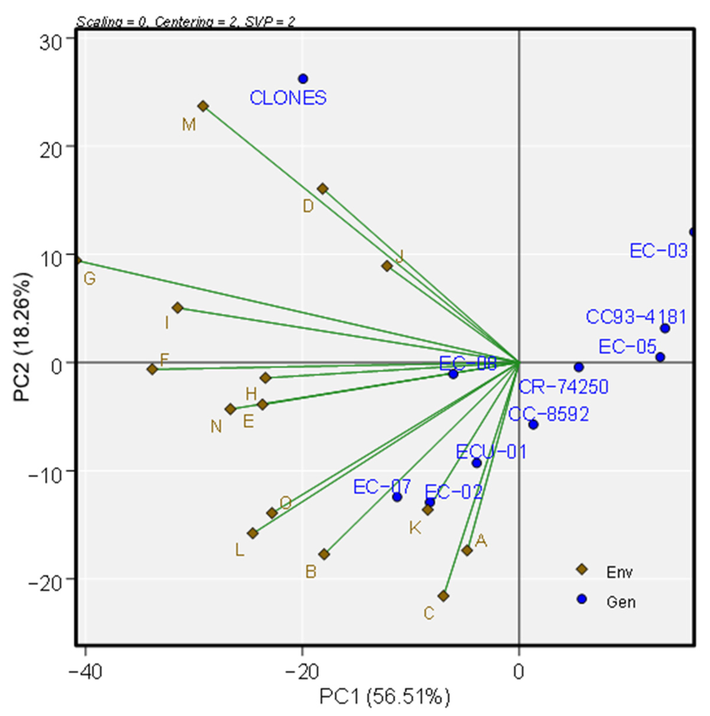
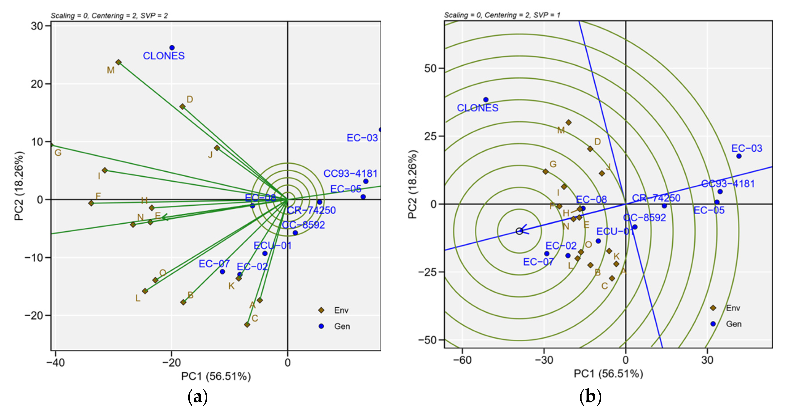
3.5. Biplot Patterns for Multivariate Analysis

Biplot patterns are divided into three main sections: the “which-won-where” pattern, based on the correlation between genotypes and environments; the “mean vs. stability” pattern, measured according to the genotype; and the “discriminative vs. representativeness” pattern, which evaluates the test environments [11,18]. These biplot patterns form a two-dimensional visualization matrix on the X and Y axes. Within this matrix, data are centered and then decomposed using singular values (SV) into GE scores (dimensionless) for the principal components, PC1 and PC2. PC1 reflects the level of performance, while PC2 indicates the stability of the genotypes [18].

The GGE biplot (“which-won-where”) in Figure 2 shows the pattern of test data across multiple environments, where the x-axis PC1 and y-axis PC2 explain 56.51% and 18.26%, respectively, of the total variation (74.77%). The genotypes furthest from the origin in various directions formed a polygon that encompassed all other genotypes, indicating that they were the best varieties in their respective sectors. The polygon was divided into four sectors when a perpendicular line was drawn from the origin to each side of the polygon, dividing the biplot into sectors by year. The 15 environments were grouped into different clusters (environment A and C as one group, environments B, K, L as another group, environments E, H, I as a third group, and finally environments F, G and D, J as independent groups), and then the suitable genotypes for each group were identified.

The winning genotype, which has the highest yield in all the environments dividing the sector, is located at the vertex. According to Yan and Tinker., (2006) [27], genotypes located at the vertices of the polygon have had the best or worst performance in one or more environments. There are five sectors with the genotypes “CLONES”, “EC-02”, “EC-03”, “EC-05”, and “EC-07” as corner or vertex genotypes. The analysis showed that the CLONES genotype had the highest yield in environments J and D, while the EC-07 genotype had the highest yield in environment B. On the other hand, the EC-08 genotype showed higher yields in more diverse environments such as E, H, I, and to a lesser extent, environments L, K, F. This pattern suggests that the target environment may consist of two different mega-environments and that different cultivars should be selected and deployed for each.

On the other hand, the GGE biplot pattern (“mean vs. stability”) selects and evaluates the ideal genotype within a single mega-environment. In this context, genotypes should be evaluated both for their average yield and their stability across different environments. Figure 3 shows the average environment coordination (AEC) of the GGE biplot, which has the following interpretation [10,11,27]:

The line with a single arrow serves as the AEC abscissa and is known as the average environment axis (AEA) which points to the genotype with the highest yield. Therefore, “CLONES” had the highest average yield, followed by “EC-07”, “EC-02”, etc., while “EC-03” had the lowest average yield.

The AEC ordinate passes through the origin of the graph and is perpendicular to the AEC abscissa, pointing to greater variability (worse stability) in any direction. Therefore, “CLONES” was very unstable, while “CR-74250” along with “EC-08” were very stable.

Finally, the GGE biplot pattern (“discrimination vs. representativeness” and “ranking by GGE”) shows the discriminative power and representativeness of the test environments, as shown in Figure 4. The concentric circles help visualize the length of the environmental vectors, which is proportional to the standard deviation within the respective environments and is a measure of the environments’ discriminative power [27]. Therefore, among the fifteen environments studied, environment G corresponding to sector 03 in the year 2018 was the most discriminative (informative) and environment J was the least discriminative. The average environment (represented by an arrow) has the average coordinates of all the test environments. In this case, AEA is the line that passes through the average environment and the origin of the biplot. A test environment with a smaller angle to the AEA is more representative of other test environments [12]; therefore, environments N, E, and H corresponding to sectors 02, 03, and 05 (during the period 2019) are the most representative, while sectors M and D are the least representative.

4. Discussion

Sugarcane yield is independently affected by the genotype type, location, and year of cultivation, indicating that multiple characteristics act synergistically in its development. Additionally, highly significant differences are observed when genotypes are cultivated in different zones (G × S), during a specific period (G × Y), and when zones and periods are distinct (S × Y). Our results demonstrate that genotypes vary in their yield in response to particular soil characteristics and changing environmental conditions over time. Studies such as those by Klomsa-ard et al., (2013) [28] and Reddy et al., (2014) [29] show that double interactions like genotype by location and genotype by sowing date are highly significant, explaining up to 58% of the variance. Additionally, interactions such as G × Y guide future agricultural trials where the evaluation informs researchers whether to include a new site to assess different genotypic responses [30].

On the other hand, a broad spectrum of combinations (G × S × Y) does not show significant differences in all cases. These results are consistent with those of Klomsa-ard et al. [29], who suggest that the non-significant triple interaction indicates that yield differences attributed to location and crop type do not interact complexly with genotypes in a statistically predictable pattern, demonstrating that one or several environments are correlated, so the genotypic responses to these locations would be similar [7,30]. In our study, we demonstrate that decoupling the factors (locations) provides more information, making at least one specific location (Sector 04) a determining factor during cultivation periods for activating certain additive genes in the varieties, causing them to respond differently in terms of yield.

The analysis of the sources of variation using the Tukey HSD technique determines that the best sugarcane variety is the CLONES group, the best location is Sector 03, and the best production year is 2020. However, the GGE biplot patterns of the “which-won-where” indicate that the yield in CLONES responds well only to the conditions presented by environments D, G, M, and with less stability in environment J, corresponding to Sectors 02, 03, 05, and 04 during 2018, respectively. This shows that during this period, the four sectors were influenced by extrinsic factors such as the reduction of hectares dedicated to this crop [31], positive, negative, and unpredictable climatic anomalies [32], and biotic and abiotic stress interactions [23] that improve the phenotypic development of this variety and affect or maintain that of others.

The mean and stability explained by the GGE biplot showed that the CLONES had high yield but high instability across several environments. Therefore, in terms of agronomic value, the genotypes ECU-01, EC-02, EC-07, or EC-08 might be the most ideal for sugarcane production. These results align with those obtained by Yadawad et al., (2023) [5], who highlighted the productive potential of two clones from breeding programs (Co 15017 and CoSnk 15102) with high yield but high instability across various environments (high values of the sum of squared deviations), emphasizing that standard varieties offer general stability in different environments.

The pattern of representativeness and discrimination shows that among all visualizations, the Ecuadorian variety EC-08 has advantages in stability (Figure 4a). However, the variety EC-07 ranks higher in the GGE biplot ranking model with better performance (Figure 4b). These results contradict the decisions made on the part of the producing sector during the 2018 sugar production decline who mostly leaned more towards the EC-08 variety [33]. Another important pattern observed in the discriminativeness vs. representativeness graph is the stability of two additional genotypes besides variety EC-08, specifically the Colombian variety CC-8592 and the Dominican variety CR-74250. However, for effective selection, an ideal genotype must exhibit both high average yield and stability [18,27]. Although these two varieties are stable, they are located at the opposite end of the graph, indicating low yield [17]. Due to this, and considering that a significant portion of the Ecuadorian economy is based on agriculture, it highlights the importance of utilizing advanced statistical models to assess genotype-environment interaction (GEI) in order to establish a more informed and precise selection of genotypes.

The yield and stability of sugarcane can be affected by the specific agricultural needs of each variety, the inherent characteristics of each genotype, as well as by soil and climate conditions [5,18]. Moreover, the interaction between individuals and their environment is determinant, even when uniform treatments of irrigation, fertilization, and integrated pest and disease management are applied [7,23]. In this study, the ANOVA and GGE analyses reveal that the genotypic effect predominates in terms of performance and stability in released varieties, whereas the environmental impact is greater in the group of clones. These findings could alert sugar companies and plant breeders, and guide future sectoral research indicating that the combination of controlling different sectors along with the management of local agricultural practices and the appropriate selection of varieties could optimize yield levels and unveil new patterns of agricultural development. We also suggest the use of GGE biplot representations because of their versatile interpretation for identifying plant materials that are resistant, stable, durable, and responsive to various conditions [16,30,34].

Despite the growing interest in the GGE biplot method as an agricultural analysis tool, this study faces certain limitations. The first limitation is linked to the sample analyzed, which comes exclusively from two major sugarcane producers in the province of Guayas, Ecuador [33]. This restricts the generalizability of our results to other regions and countries. This goes hand in hand with our second limitation, arising from the lack of access to more varied data, which restricted our ability to analyze a model that includes different types of agricultural practices, levels of technification, or sugarcane producers with varying levels of production, factors that could reveal patterns not observed in this study.

Our results highlight the diversity of responses among sugarcane varieties. However, further analysis of these patterns is necessary to improve the questionable sustainability of this crop, especially in the province of Guayas [3,31]. Although practices carried out during harvest and processing, such as CO₂ emissions, and social factors like the satisfaction and acceptability of the production system, do not pose alarming problems, the sustainability index at the economic and ecological levels reveals deficiencies [35,36]. These include limitations in production diversification, a high dependency on external inputs, and practices that compromise soil conservation, such as chemical fertilization and crop burning [36].

Finally, a third limitation is related to the period analyzed (2018–2020). Due to the longitudinal nature of the study, new varieties are released each year that are adopted by different producers [4,33]. In this sense, the inability to analyze the stability and performance of varieties over a broader time frame (e.g., 2018–2023) limits our capacity to capture all the desired effects on sugarcane agricultural practices over time.

5. Conclusions

This research revealed that the sugarcane varieties in the study exhibit varied phenotypic expressions, indicating that the individuals are genetically distinct from each other. This demonstrates that the varieties produced in the country exhibit high variability and have considerable potential for successful cultivation. The genotypic variation in yield revealed significant interactions of the G × S (genotype by sector) and G × Y (genotype by year) effects, as well as a significant effect of the triple interaction G × S × Y. This latter interaction indicates that one of the sectors may induce distinctive responses among the genotypes. Regarding specific varieties, the clones selected for the study generally showed high yield in most locations; however, this high yield was particularly notable during the 2018 period, suggesting that these varieties are especially suitable for the specific environmental conditions of that year. Among the varieties that showed greater stability, the Ecuadorian varieties EC-07 and EC-08, as well as the Colombian CC-8502 and the Dominican CR-74250, stand out. However, EC-07 showed the highest yield with slight instability, contrasting with the two foreign varieties that showed a notable reduction in yield compared to all Ecuadorian varieties, suggesting that adaptability and improvement opportunities may be more promising in specific geographic areas with similar agricultural needs.

References

1. Lee, H.; Sohn, Y.J.; Jeon, S.; Yang, H.; Son, J.; Kim, Y.J.; Park, S.J. Sugarcane wastes as microbial feedstocks: A review of the biorefinery framework from resource recovery to production of value-added products. Bioresour. Technol. 2023, 376, 128879. [Google Scholar] [CrossRef]
2. Ministerio de Agricultura y Ganadería (MAGAP). Luego de Siete años Aumenta el Precio de la Tonelada de Caña de Azúcar. Available online: https://www.agricultura.gob.ec/luego-de-siete-anos-aumenta-el-precio-de-la-tonelada-de-cana-de-azucar (accessed on 8 July 2024).
3. INEC (Instituto Nacional de Estadística y Censo). Encuesta de Superficie y Producción Agropecuaria Continua. ESPAC. 2022. Available online: https://www.ecuadorencifras.gob.ec/encuesta-de-superficie-y-produccion-agropecuaria-continua-2022/ (accessed on 8 July 2024).
4. Silva, E.; Martínez, F.; Madrid, C.; León, T.; Castillo, R.; Mendoza, J.; Garcés, F.; Salazar, M.; Aucatoma, B.; Fiallos, B.; et al. EC-07 y EC-08, nuevas variedades mejoradas de caña de azúcar. Boletín Divulg. 2016, 10, 1–9. [Google Scholar]
5. Yadawad, A.; Patil, S.B.; Kongawad, B.Y.; Kadlag, A.D.; Hemaprabha, G. Multi environmental evaluation for selection of stable and high yielding sugarcane (Saccharum officinarum L.) clones based on AMMI and GGE biplot models. Indian. J. Genet. Plant Breed. 2023, 83, 389–397. [Google Scholar] [CrossRef]
6. Natarajan, S.; Basnayake, J.; Lakshmanan, P.; Fukai, S. Limited contribution of water availability in genotype-by-environment interaction in sugarcane yield and yield components. J. Agron. Crop Sci. 2020, 206, 665–678. [Google Scholar] [CrossRef]
7. Dang, X.; Hu, X.; Ma, Y.; Li, Y.; Kan, W.; Dong, X. AMMI and GGE biplot analysis for genotype × environment interactions affecting the yield and quality characteristics of sugar beet. PeerJ 2024, 12, e16882. [Google Scholar] [CrossRef]
8. Oladosu, Y.; Rafii, M.Y.; Abdullah, N.; Magaji, U.; Miah, G.; Hussin, G.; Ramli, A. Genotype × Environment interaction and stability analyses of yield and yield components of established and mutant rice genotypes tested in multiple locations in Malaysia. Acta Agric. Scand. B Soil Plant Sci. 2017, 67, 590–606. [Google Scholar] [CrossRef]
9. Liu, Q.; Huang, L.; Fu, C.; Zhang, T.; Ding, W.; Yang, C. Genotype–environment interaction of crocin in Gardenia jasminoides by AMMI and GGE biplot analysis. Food Sci. Nutr. 2022, 10, 4080–4087. [Google Scholar] [CrossRef]
10. Yan, W.; Cornelius, P.L.; Crossa, J.; Hunt, L.A.; Yan, W. Two Types of GGE Biplots for Analyzing Multi-Environment Trial Data. Crop Sci. 2001, 41, 656–663. [Google Scholar] [CrossRef]
11. Yan, W.; Hunt, L.A.; Sheng, Q.; Szlavnics, Z. Cultivar Evaluation and Mega-Environment Investigation Based on the GGE Biplot. Crop Sci. 2000, 40, 597–605. [Google Scholar] [CrossRef]
12. Frutos, E.; Galindo, M.P.; Leiva, V. An interactive biplot implementation in R for modeling genotype-by-environment interaction. Stoch. Env. Res. Risk Assess. 2014, 28, 1629–1641. [Google Scholar] [CrossRef]
13. Gabriel, K.R. The biplot graphic display of matrices with application to principal component analysis. Biometrika 1971, 58, 453–467. [Google Scholar] [CrossRef]
14. Galindo-Villardón, P. Una Alternativa de Representación Simultánea: HJ-Biplot. Qüestiió 1986, 10, 13–23. [Google Scholar]
15. Mehareb, E.M.; Osman, M.A.M.; Attia, A.E.; Bekheet, M.A.; Fouz, A.E.F.M. Stability assessment for selection of elite sugarcane clones across multi-environment based on AMMI and GGE-biplot models. Euphytica 2022, 218, 95. [Google Scholar] [CrossRef]
16. Maulana, H.; Solihin, E.; Trimo, L.; Hidayat, S.; Wijaya, A.A.; Hariadi, H.; Amien, S.; Ruswandi, D.; Karuniawan, A. Genotype-by-environment interactions (GEIs) and evaluate superior sweet potato (Ipomoea batatas [L.] Lam) using combined analysis and GGE biplot. Heliyon 2023, 9, e20203. [Google Scholar] [CrossRef]
17. Esan, V.I.; Oke, G.O.; Ogunbode, T.O.; Obisesan, I.A. AMMI and GGE biplot analyses of Bambara groundnut [Vigna subterranea (L.) Verdc.] for agronomic performances under three environmental conditions. Front. Plant Sci. 2023, 13, 997429. [Google Scholar] [CrossRef]
18. Khan, M.M.H.; Rafii, M.Y.; Ramlee, S.I.; Jusoh, M.; Al Mamun, M. AMMI and GGE biplot analysis for yield performance and stability assessment of selected Bambara groundnut (Vigna subterranea L. Verdc.) genotypes under the multi-environmental trials (METs). Sci. Rep. 2021, 11, 22791. [Google Scholar]
19. Yan, W. Singular-Value Partitioning in Biplot Analysis of Multienvironment Trial Data. Agron. J. 2002, 94, 990–996. [Google Scholar]
20. Akan, K.; Cat, A.; Hocaoglu, O.; Tekin, M. Evaluating Scald Reactions of Some Turkish Barley (Hordeum vulgare L.) Varieties Using GGE Biplot Analysis. Agronomy 2023, 13, 2975. [Google Scholar] [CrossRef]
21. Zhao, F.; Li, Y.; Cui, T.; Bai, J. GGE Biplot-Based Transcriptional Analysis of 7 Genes Involved in Steroidal Glycoalkaloid Biosynthesis in Potato (Solanum tuberosum L.). Agronomy 2023, 13, 2127. [Google Scholar] [CrossRef]
22. Valenzuela-Cobos, J.D.; Guevara-Viejó, F.; Vicente-Galindo, P.; Galindo-Villardón, P. Eco-Friendly Biocontrol of Moniliasis in Ecuadorian Cocoa Using Biplot Techniques. Sustainability 2023, 15, 4223. [Google Scholar] [CrossRef]
23. Mehdi, F.; Cao, Z.; Zhang, S.; Gan, Y.; Cai, W.; Peng, L.; Wu, Y.; Wang, W.; Yang, B. Factors affecting the production of sugarcane yield and sucrose accumulation: Suggested potential biological solutions. Front. Plant Sci. 2024, 15, 1374228. [Google Scholar] [CrossRef]
24. Ellis, R.N.; Basford, K.E.; Cooper, M.; Leslie, J.K.; Byth, D.E. A methodology for analysis of sugarcane productivity trends. I. Analysis across districts. Aust. J. Agric. Res. 2001, 52, 1001–1009. [Google Scholar] [CrossRef]
25. Zhang, H.; Feng, Z.; Wang, J.; Yun, X.; Qu, F.; Sun, C.; Wang, Q. Genotype by environment interaction for grain yield in foxtail millet (Setaria italica) using AMMI model and GGE Biplot. Plant Growth Regul. 2022, 99, 101–121. [Google Scholar] [CrossRef]
26. Yan, W.; Kang, M.S. GGE Biplot Analysis: A Graphical Tool for Breeders, Geneticists, and Agronomists. GGE Biplot Analysis [Internet]. 28 August 2002. Available online: https://www.taylorfrancis.com/books/mono/10.1201/9781420040371/gge-biplot-analysis-weikai-yan-manjit-kang (accessed on 9 July 2024).
27. Yan, W.; Tinker, N.A. Biplot analysis of multi-environment trial data: Principles and applications. Can. J. Plant Sci. 2006, 86, 623–645. [Google Scholar] [CrossRef]
28. Klomsa-ard, P.; Jaisil, P.; Patanothai, A. Performance and Stability for Yield and Component Traits of Elite Sugarcane Genotypes Across Production Environments in Thailand. Sugar Tech 2013, 15, 354–364. [Google Scholar] [CrossRef]
29. Reddy, P.S.; Reddy, B.V.S.; Rao, P.S. Genotype by sowing date interaction effects on sugar yield components in sweet sorghum (Sorghum bicolor L. moench). SABRAO J. Breed. Genet. 2014, 46, 305–312. [Google Scholar]
30. Shojaei, S.H.; Mostafavi, K.; Ghasemi, S.H.; Bihamta, M.R.; Illés, Á.; Bojtor, C.; Nagy, J.; Harsányi, E.; Vad, A.; Széles, A.; et al. Sustainability on Different Canola (Brassica napus L.) Cultivars by GGE Biplot Graphical Technique in Multi-Environment. Sustainability 2023, 15, 8945. [Google Scholar] [CrossRef]
31. Orbe, D.; Cuichán, M. Encuesta de Superficie y Producción Agropecuaria Continua; INEC (Instituto Nacional de Estadística y Censos): Loja, Ecuador, 2022; pp. 2–14. [Google Scholar]
32. de Guenni, L.B.; García, M.; Muñoz, G.; Santos, J.L.; Cedeño, A.; Perugachi, C.; Castillo, J. Predicting monthly precipitation along coastal Ecuador: ENSO and transfer function models. Theor. Appl. Climatol. 2017, 129, 1059–1073. [Google Scholar] [CrossRef]
33. Silva, E.; Madrid, C.; Martínez, F.; León, T. Programa de variedades. In Centro de Investigación de la Caña de Azúcar (CINCAE), Informe Anual 2021; El Triunfo, Ecuador, 2022; pp. 2–10. Available online: https://cincae.org/wp-content/uploads/2022/06/Informe-Anual-2021.pdf (accessed on 2 June 2024).
34. Melios, S.; Ninou, E.; Irakli, M.; Tsivelika, N.; Sistanis, I.; Papathanasiou, F.; Didos, S.; Zinoviadou, K.; Karantonis, H.C.; Argiriou, A.; et al. Effect of Genotype, Environment, and Their Interaction on the Antioxidant Properties of Durum Wheat: Impact of Nitrogen Fertilization and Sowing Time. Agriculture 2024, 14, 328. [Google Scholar] [CrossRef]
35. Bucarám Ortíz, J.; Garcia, Y.; Vega, A.; Amador Sacoto, C.; Borodulina, T.; Mancero-Castillo, D. Dynamics of co2 emission and dispersion from two sugarcane mills in the Guayas basin. Chilean J. Agric. Anim. Sci. 2023, 39, 296–304. [Google Scholar] [CrossRef]
36. Amador-Sacoto, C.; Helfgott-Lerner, S. Sustainability of Sugarcane Farms in the Milagro Canton, Ecuador. Int. J. Adv. Sci. Eng. Inf. Technol. 2023, 13, 837–843. [Google Scholar] [CrossRef]
Figure 1. GGE biplot.
Applsci 14 06665 g001
Figure 2. Which-on-where.
Applsci 14 06665 g002
Figure 3. Mean vs. Stability.
Applsci 14 06665 g003
Figure 4. Discriminativeness vs. representativeness and ranking genotypes: (a) shows the stability of genotypes and environments; (b) shows the rankings generated by the GGE model.
Applsci 14 06665 g004