Application Study of the High-Strain Direct Dynamic Testing Method

Abstract

The high-strain direct testing method is a novel technique for dynamic testing of pile bearing capacity, developed as an improvement to the traditional high-strain method. While its theoretical feasibility has been demonstrated through numerical simulations and laboratory experiments, its effectiveness in practical engineering applications remains uncertain. This paper discusses the foundational theory of the high-strain direct testing method, highlighting its clear calculation principles, straightforward process, and advantage of not requiring iterative fitting. The bridge project in Zhuhai, Guangdong Province, China, serves as a case study. An instrumentation layout for concrete-filled piles was designed based on the principles of the high-strain direct testing method, and data processing and analysis programs were developed using Python. Fifteen test piles were selected for field application of the high-strain direct testing method, with detailed analysis conducted on the results from four test piles. The test results were consistent with the soil layer distribution characteristics beneath the four piers of the bridge, validating the feasibility of this method in actual engineering practice. Subsequent static load tests on these four test piles allowed for a comparison with the high-strain direct testing method results, confirming the accuracy and reliability of the high-strain direct testing method for determining the bearing capacity of single piles. Furthermore, this paper identifies sources of error in the application of this method and proposes corresponding improvement measures. As this method directly derives results from instrumented measurements, it is theoretically applicable to piles of any cross-sectional shape and material, provided that enough measurement lines can be successfully arranged along the pile shaft. This capability allows for the real-time estimation of the ultimate bearing capacity during pile driving, thereby enhancing the universality of the high-strain direct dynamic testing method beyond traditional techniques.

1. Introduction

In the field of foundation engineering, one of the key indicators for assessing the quality of a pile foundation is verifying whether its bearing capacity meets the requirements of design criteria. Currently, there are two main methods for evaluating the bearing capacity of pile foundations, which include the following: the static load test and the high-strain dynamic test. In the static load test, loads are incrementally applied to the pile top, and the bearing capacity of the individual pile is determined by the relationship between pile top displacement and the applied load [1,2,3,4]. The high-strain dynamic test involves applying impact loads to the pile top using a heavy hammer to induce sufficient relative displacement between the pile and the soil. One-dimensional wave theory is then applied to analyze the reflected stress waves from the pile toe, thus determining the bearing capacity of the individual pile. The static load test has long been considered to be the standard method for assessing the bearing capacity of piles because of its straightforwardness and accuracy. However, this method is time-consuming, expensive, and often limited by geographical constraints. In contrast, the high-strain dynamic test has numerous advantages, such as lightweight equipment, a shorter testing time, lower costs, and a wider range of applicable situations. Consequently, this method has been rapidly adopted since its inception.

The core principle of the high-strain dynamic testing method is to analyze the stress wave-by-wave theory within the pile during the driving process. In 1931, [5] first proposed that a one-dimensional wave equation can be applied to the practical application of stress wave theory. In 1960, [6] proposed a model representing the pile driving system using a series of mass blocks, springs, and dampers to simulate the hammer, pile, and soil. This model was solved using numerical difference methods. To better characterize the soil’s resistance to the pile, he introduced two new parameters as follows: the soil’s elastic limit and the damping coefficient. The analysis model, solution method, and parameters introduced by Smith established the theoretical foundation for modern high-strain dynamic testing methods.

The practical application of the high-strain dynamic method in engineering primarily stems from the work of [7,8,9,10,11,12,13,14,15] at Case Western Reserve University. Their invention, the Pile Driving Analyzer (PDA), transformed academic research into a process that the engineering community embraced. They also developed an analytical method called CAPWAP (Case Pile Wave Analysis Program) with the advent of digital computation. CAPWAP fits the calculated force curve to the measured force curve by making reasonable assumptions about the pile–soil model’s parameters, ultimately determining the load-bearing capacity using the set of parameters that achieve the best fit. However, different sets of parameters can potentially yield the same fit, resulting in multiple possible solutions, which introduces ambiguity into the method.

In 1980, the first international seminar on “The Application of Stress-Wave Theory to Piles” was held, promoting research on the high-strain method in multiple countries. Over the subsequent decades, researchers proposed a series of improved models [15,16,17,18,19], and extensive studies were conducted on the pile–soil interaction mechanism under impact loads [20,21,22,23,24]. In addition, the use of machine learning to describe the geomaterial heterogeneity is included in the numerical modeling methods [25]. With technological advancements, artificial intelligence has been integrated into pile-bearing capacity prediction models. For instance, Chen et al. [26] applied genetic programming (GP) to enhance efficiency in predicting ultimate pile capacity, while Duan et al. [27] combined machine learning (ML) with advanced optimization algorithms to improve prediction accuracy, developing three predictive models. These efforts yielded significant findings, making the high-strain method increasingly routine in pile foundation testing. The improved models offered clearer physical insights and better descriptions of the complex mechanical responses of the soil during pile driving. However, with the increase in parameters, these models became more complex and often difficult to implement in practical engineering applications.

The key to applying the high-strain method for testing the load-bearing capacity of foundation piles lies in determining the soil resistance model and its corresponding parameters. Yuan and Zhu [28] highlighted the need to restrict fitting parameter ranges to address the uniqueness problem in common soil resistance models. In addition, the actual accuracy and application scope of high-strain dynamic pile testing, noting discrepancies, uncertainties in CAPWAP signal matching, negligible effects of soil properties on results, and potential misinterpretations, were discussed, as clearly explained in [29,30]. Verbeek et al. [31] found that for multi-layer soils with many parameters, fitting often relies heavily on the analyst’s subjective judgment, introducing significant subjectivity.

To address these issues, Zhu and Zhang [32] proposed a new method for dynamic testing of pile load-bearing capacity under high-strain conditions. Unlike traditional methods, this approach involves placing more strain sensors at various depths along the pile shaft. After a heavy hammer impacts the pile, these sensors accurately capture strain data at each measurement point. Based on these empirical data, the ultimate load-bearing capacity of the entire pile can be determined. This calculation model is straightforward and intuitive, avoiding the need for complex soil resistance models and allowing for direct calculation of the pile’s ultimate load-bearing capacity. Thus, it is termed the “high-strain direct dynamic testing method.”

Currently, research on this method is limited to theoretical analysis [33] and laboratory experiments [34]. Its effectiveness and reliability in actual projects have yet to be validated. Additionally, the sources and ranges of errors in using this method to test the load-bearing capacity of individual piles in engineering practice are not yet clear. Given that this method requires numerous strain sensors to be installed along the pile shaft, efficient sensor placement remains a technical challenge in practical applications.

In previous studies, researchers mainly evaluated the accuracy of the high-strain method by comparing dynamic and static load test results [35,36,37,38]. Although the high-strain direct dynamic method has improved computational principles over traditional methods, making bearing capacity predictions more direct, static load test results remain the benchmark for evaluating the reliability of dynamic testing results.

The objective of this paper concerns the ability to use the high-strain direct dynamic method in engineering practice. The first part of this research focuses on explaining the basic principles of the arrangement of measurement instruments. The second part calculates the ultimate bearing capacity of a single pile using measured data. In the current research, the bridge project founded in Guangdong Province, China, was taken as a case study to apply the methods of the high-strain direct dynamic method under field conditions. To verify the method’s reliability in detecting single pile-bearing capacity, static load tests were designed and implemented on selected test piles, using the results as a base for evaluating the accuracy of the dynamic test results. The error range and possible sources of error between the high-strain direct dynamic method and the static load test were compared and analyzed.

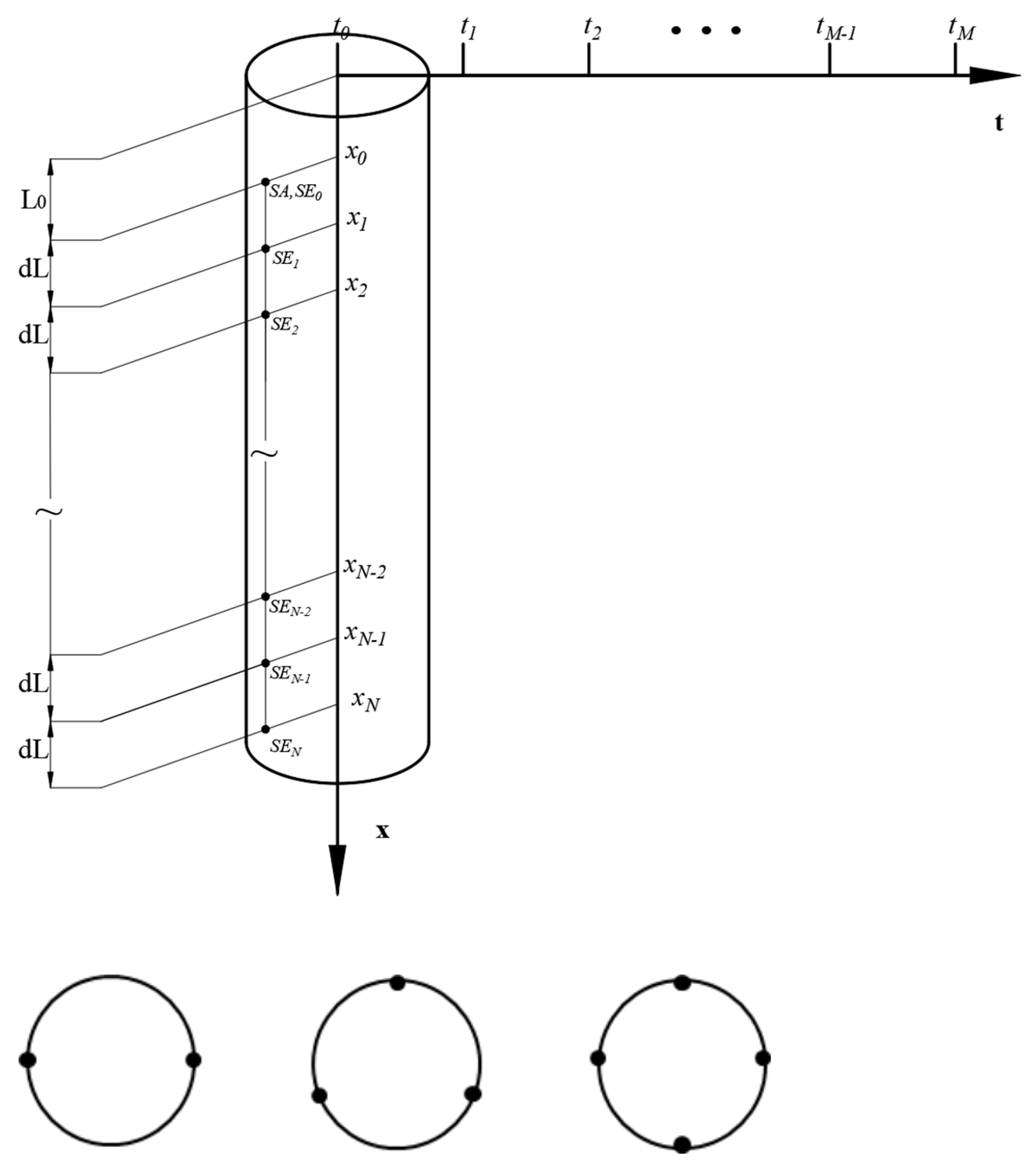
2. Theory of the High-Strain Direct Dynamic Testing Method

2.1. Measuring Instruments

For a foundation pile with length L and diameter D, as shown in Figure 1, the pile top center is taken as the origin of coordinates, and the x-axis is established along the pile shaft direction, with time t as the horizontal axis. Strain sensors are installed at positions with depth x, with N + 1 strain sensors in total. The strain sensor at depth should be as close to the pile bottom as possible to reflect the actual end-bearing force more accurately. The arrangement of strain sensors along the pile shaft should be based on the distribution of soil layers on-site. For this study, the sensor placement was conducted following the Code for Testing of Building Foundation (DBJ/T 15-60-2019) [39].

A complete measurement line is formed by the pile top accelerometer SA. Many strain sensors are used, one at the pile top and the rest at nodes distributed at various depths along the pile shaft. Each measurement line should be parallel to the central axis of the pile and evenly distributed across the pile’s cross-section.

The piling equipment and impact on the pile top with a hammer after setting the sampling interval $dt$ for the testing instruments are activated, with a total of M samples collected. The mass of the hammer, the impact method, the sampling interval dt, and the number of samples M should all agree with relevant standards and specifications.

2.2. Basic Assumptions

When calculating the ultimate bearing capacity of a single pile using the high-strain direct dynamic method, the pile is discretized into a series of pile segments at the nodes where strain sensors are placed along the pile shaft as shown in Figure 2. The ultimate bearing capacity of the pile equals the sum of the ultimate static soil resistance acting on each pile segment. The basic assumptions of this method are summarized as follows:

1—The total soil resistance around the pile during longitudinal vibration under dynamic load consists of static and dynamic resistances. Static resistance is related to the relative displacement between the pile and soil, while dynamic resistance is related to the pile’s velocity.

2—When the average velocity of a pile segment is zero, its dynamic resistance is zero.

3—When the dynamic resistance of a pile segment first drops to zero from its peak value, the total soil resistance on that pile segment is considered to have reached the segment’s lateral ultimate static resistance.

2.3. Computation Theory

For sensors $x_n(n\in \left[0,N\right])$ at any given depth, the average strain ${ϵ}_{i,j}$ and average acceleration $a_{i,j}$ of the pile cross-section at that depth are obtained by averaging the measured data from each row of the measurement lines (the subscript $i$ represents position and the subscript j represents time).

When $j=0$, $t=dt‧ j=0$, it indicates that pilling has not begun, and at this moment, all the variables are zero. When $j>0$, it indicates that the hammer impacted the pile top, and at this moment, by performing a single integration of the pile top acceleration ${\alpha }_{0,j}$ over, the velocity $dt$ of the pile top can be obtained. A second integration yields the displacement $u_{o,j}$.

$$v_{0,j+1}=v_{0,j}+{\displaystyle \frac{(a_{0,j}+a_{0,j+1})}{2}}dt$$

(1)

$$u_{0,j+1}=u_{0,j}+{\displaystyle \frac{(v_{0,j}+v_{0,j+1})}{2}}dt$$

(2)

where $j\in \left[0,M-1\right]$.

$v_{0,j+1},v_{0,j}=$ the velocity of sensor $x_0$ at the moment $\mathrm{t}\mathrm{i}\mathrm{m}\mathrm{e}=j+1$ and $\mathrm{t}\mathrm{i}\mathrm{m}\mathrm{e}=j$.

$a_{0,j+1},a_{0,j}=$ the acceleration of sensor $x_0$ at the moment $\mathrm{t}\mathrm{i}\mathrm{m}\mathrm{e}=j$ and $\mathrm{t}\mathrm{i}\mathrm{m}\mathrm{e}=j$.

$u_{0,j}=$ the displacement of sensor $x_0$ at the moment $\mathrm{t}\mathrm{i}\mathrm{m}\mathrm{e}=j$.

However, measurement devices typically have zero-offset errors, leading to significant cumulative errors in time integration of acceleration. This error can be corrected using the actual settlement value of the pile top ${ L}_0$ measured at the end of the test. Where the measured settlement value at the end of sampling is $P_d$ and the difference between the calculated displacement $u_{o,j }$ by twice integrating the acceleration and ${ P}_d$ is $s_d$. Then, the displacement can be corrected using the following equations:

$$U_{0,j=u_{0.j}-u_{0,j}-s_d}.{\displaystyle \frac{j}{M}}=u_{0,j}-\left(u_{0,j}{P}_d\right).{\displaystyle \frac{j}{M}}$$

(3)

where $j\in \left[0,M-1\right]$.

The corrected velocity $V_{0,j}$ can be obtained by differentiating the corrected displacement $U_{0,j}$ once with respect to the sampling time interval. Similarly, the corrected acceleration $A_{0,j}$:

$$\begin{gathered} V_{\mathrm{0,0}}=0 \\ {V}_{0,j}={\displaystyle \frac{U_{0,j}-U_{0,j-1}}{dt}} \end{gathered}$$

(4)

$$\begin{gathered} A_{\mathrm{0,0}}=0 \\ {A}_{0,j}={\displaystyle \frac{V_{0,j}-V_{0,j-1}}{dt}} \end{gathered}$$

(5)

where $j\in \left[0,M\right]$.

Then, the corrected displacement of the pile top $U_{o,j }$, combined with the measured average strain ${ϵ}_{i,j}$ along the pile body, can be used to derive the displacement $u_{i,j}$ at any depth nodes along the pile:

$$u_{i,j}=u_{i-1,j}+{\displaystyle \frac{\left({ϵ}_{i,j}+{ϵ}_{i-1,j}\right)}{2}}(x_i-x_{i-1})$$

(6)

where $i\in \left[1,N\right]$; $j\in \left[1,M-1\right]$.

Based on the displacement $u_{i,j}$ obtained for each depth node along the pile body, the velocity $v_{i,j}$ at each node can be calculated using difference formulas. Subsequently, the acceleration $a_{i,j}$ at each node can be determined from these velocity values:

$$v_{i,j}={\displaystyle \frac{u_{i,j}-u_{i,j-1}}{dt}}$$

(7)

$$a_{i,j}={\displaystyle \frac{v_{i,j}-v_{i,j-1}}{dt}}$$

(8)

where $i\in \left[1,N\right]$; $j\in \left[1,M-1\right]$.

For a chosen sampling time interval $dt$, the axial force in the pile body at each depth node can be calculated using the measured average strain ${ϵ}_{i,j}$ at that node, as the following equation:

$$F_{i,j}=-E\times A\times {ϵ}_{i,j}$$

(9)

where E is the elastic modulus of the pile, $E=\rho c^2$, $\rho$ is the density of the pile, and c is the wave velocity of the stress wave within the pile. A is the cross-sectional area of the pile. In this paper, compressive stress is considered positive, while tensile strain is considered negative.

Using the above equations, the axial force $F_{i,j}$ and acceleration $a_{i,j}$ at each depth node of the pile can be calculated. For any pile segment between two adjacent nodes $x_i$ and $x_{i+1}$, a force analysis can be conducted, as shown in Figure 3. Based on the basic assumptions of this method, the dynamic resistance $R_{dt,j}$ experienced by this pile segment at any given time can be determined as follows:

$$R_{dt,j}=F_{i,j}-F_{i+1,j}-m_i{a}_i=F_{i,j}-F_{i+1,j}-\rho A{\displaystyle \frac{\left(x_{i+1}{x}_i\right)}{2}}(a_{i,j}+a_{i+1,j})$$

(10)

where $i\in \left[0,N-1\right]$; $j\in \left[0,M-1\right]$.

According to the basic assumptions of this method, the total soil resistance R during the vibration of any pile segment unit is composed of static soil resistance $R_S$ and dynamic soil resistance $R_d$. Affected by the soil resistance, the vertical vibration of the pile segment will decrease over time to a relatively static state. Therefore, the displacement of the pile segment unit reaches its peak value at the moment when the initial velocity drops to zero. In addition, the dynamic resistance of the pile segment also drops to zero and the static soil resistance at this moment will also reach its maximum.

For a certain pile section with node depths from $x_i$ to $x_{i+1}$ in the pile, the average velocity of the pile section at any time can be calculated from the velocities of the upper and lower nodes:

$${\overline{v}}_{i,j}={\displaystyle \frac{(v_{i,j}+v_{i+1,j})}{2}}$$

(11)

where $i\in \left[0,N-1\right]$; $j\in \left[1,M\right]$.

At the moment of the first time ${\overline{v}}_{i,j}$ = 0, the dynamic resistance $R_{dt,j}$ at the moment obtained by Equation (10) is the pile side ultimate static resistance of this pile segment. By adding the lateral ultimate static resistance of each pile segment, the lateral ultimate static resistance of the entire pile body $R_S$ can be obtained as:

$$R_s={\sum }_{i=0}^{N-1}{R}_{si}$$

(12)

For the pile segment unit located at the bottom of the pile, after obtaining the moment $t=j$ when $v_{N,i}=0$, the axial force $F_{N,i}$ calculated at the moment is regarded as the ultimate static resistance $R_b$ of this pile segment unit.

In summary, the ultimate bearing capacity R of a single pile is the sum of the ultimate static resistance of the pile side $R_s$ and the ultimate static resistance of the pile end $R_b$:

$$R=R_s+R_b$$

(13)

The high-strain direct dynamic testing method utilizes strain sensors distributed at various depths along the pile shaft and an accelerometer positioned at the pile head to directly determine the ultimate bearing capacity of a single pile based on the results of field hammer impact tests. The calculated bearing capacity is influenced solely by the material properties and dimensions of the pile itself.

This method avoids the impact on the objectivity and reliability of results caused by relying on the experience of testers to select pile–soil interaction parameters, as seen in traditional techniques. Based on solving straightforward dynamic equilibrium equations, this method eliminates the need for the cumbersome steps of repeatedly solving and fitting the upward reflective wave from the pile base, thereby addressing the issue of multiple solutions present in traditional techniques.

3. High-Strain Direct Dynamic Test and Static Load Test

3.1. Engineering Background and Ground Investigation

This paper uses a bridge project in Zhuhai City, Guangdong Province, China, as a case study. The proposed site for this project is located upstream of a river. Therefore, the pile foundation must penetrate through a thick layer of soft clay and embed into the moderately weathered rock layer to support the bridge’s superstructure. There are four arch bases beneath the bridge. Arch bases 1 to 3 utilize nine straight bored piles with a diameter of 2.2 m and three inclined steel pipe piles with a diameter of 1.5 m (inclined at 7 degrees). While arch base #4 employs twenty-four straight bored piles with a diameter of 2.2 m and fourteen inclined steel pipe piles with a diameter of 1.5 m (inclined at 7 degrees). The foundation piles are designed as rock-socketed piles, requiring an embedment into the moderately weathered granite of no less than 2D. The reinforcement for the piles uses HRB400φ32 main bars, and the concrete used is C30 underwater concrete. The design parameters of the foundation piles are shown in

Table 1. Pile design parameters.

Material	Diameter (m)	Elastic Modulus GPa	Poisson’s Ratio	Bulk Density kN/m3
C30	2.2	34	0.2	24

.

In routine traditional high-strain testing for pile quality, random sampling is typically employed at the project site. In this study, 15 straight test piles were randomly selected for hammer impact testing. Initial data collected from on-site testing equipment revealed that some test piles did not yield complete or valid data. This issue was primarily due to the loosening or damage of the Fiber Bragg Grating (FBG) sensors during concrete pouring in certain piles. Additionally, some test piles experienced eccentric hammer impacts, resulting in significant deviations and invalid data.

To address this, the most complete and valid test pile from each of the four arch bases was selected for detailed analysis and to conduct static load tests. The analysis focuses on these four test piles, identified as #1–5, #2–7, #3–9, and #4–17. Basic information about these four test piles is presented in

Table 2. Characteristic values of the bearing capacity of the test piles.

Pile No.	Diameter (mm)	Length (m)	Concrete Strength Grade	Vertical Designed Bearing Capacity of Single Pile (kN)	Vertical Allowable Bearing Capacity of Single Pile (kN)
1–5	2200	34	C30	4755	≥9510
2–7	2200	42.5	C30	4344	≥8688
3–9	2200	48	C30	4701	≥9402
4–17	2200	68	C30	5580	≥11,160

.

It is worth noting that the region features of Zhuhai City, Guangdong Province, extensive coastal plains with alluvial soils. These areas are typically characterized by soft, silty, and clayey soils deposited by rivers and tidal actions, which can pose challenges for construction because of their compressibility and potential for settlement. Therefore, accurate assessment of soil parameters often requires a comprehensive approach to drilling sampling and in situ testing. Based on the geological age, origin, and physical–mechanical properties of the foundation soil, along with the results from geotechnical tests and in situ test indicators, and integrating regional experience, the recommended geotechnical parameters for each rock and soil layer are provided in

Table 3. Geotechnical parameter recommendation table.

Layer	Soil Layer Type	Compression Modulus K (MPa)	Poisson’s Ratio	Bulk Density (kN/m3)	Cohesion (kPa)	Friction Angle (°)	Water Content (%)	Allowable Value of Foundation Bearing Capacity fao (kPa)
A	Filled soil	8.19	0.31	20.3	-	23.8	18.2	75
B	Silt	1.53	0.34	15.1	2.2	1.6	75.9	40
C	Clay	2.20	0.34	16.5	7.1	6.1	52.5	60
D	Coarse sand	10.87	0.30	20.0	-	27.6	15.7	150
E	Sandy clay	5.28	0.22	18.8	22.4	23.4	26.4	220
F	Strongly weathered rock	5.29	0.24	18.7	23.3	28.1	26.3	300
G	Moderately weathered rock	Uniaxial compressive strength value $f_{rk}=29.9 \mathrm{M}\mathrm{P}\mathrm{a}$						650

. The soil profiles revealed by site drilling beneath the four arch bases are illustrated in Figure 4.

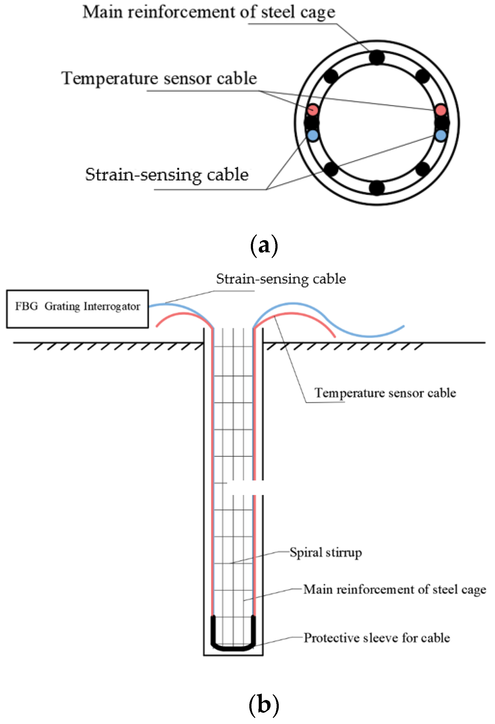
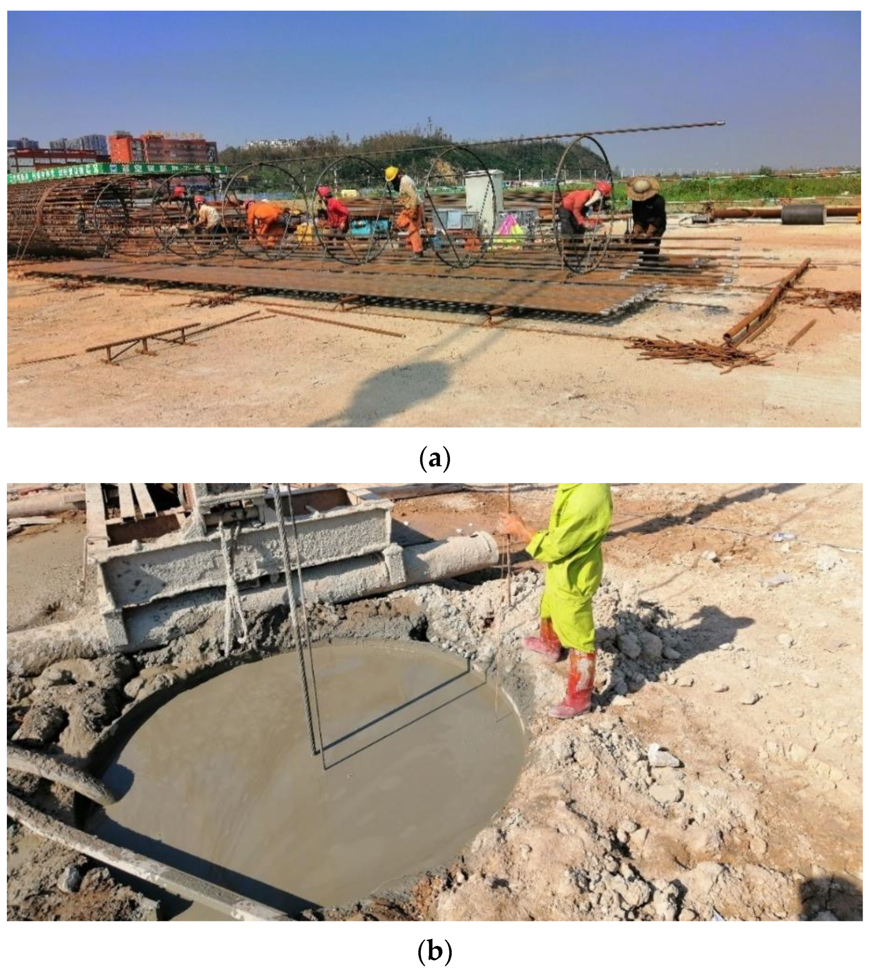
3.2. Experimental Setup

According to the instrumentation setup methods described in Section 2, each test pile was equipped with two piezoelectric strain sensors and two accelerometers, symmetrically installed at the pile top through boreholes. Additionally, a Fiber Bragg Grating (FBG) with 2 m fixed intervals was symmetrically fixed in a “U” shape to the main bars of the rebar cage before concrete pouring. Because of the high-temperature sensitivity of the FBG, temperature compensation was required for the measured strain, and thus fiber optic temperature sensors were simultaneously installed. The sensing fiber was fixed at 50 cm intervals and embedded into the concrete-filled pile, ensuring that the fiber deformation was consistent with the pile concrete deformation. Protective casings were used to safeguard the fiber sensors at the pile top and bottom during installation. A schematic diagram of the fiber optic sensor layout is shown in Figure 5.

Figure 6 presents the on-site construction drawings. In addition to the aforementioned measurement instruments, the dynamic load test was also equipped with a high-strain dynamic tester and a high-dynamic Fiber Bragg Grating (FBG) demodulator. These devices were connected to the strain sensors and accelerometers at the pile top, as well as the FBG sensors within the pile. Both instruments were configured with a sampling interval of dt = 200 μs, recording M = 1024 sampling data points. A 12-ton pile hammer was used to apply instantaneous dynamic loads to the pile top, selected according to local code [38]. Additionally, a 10 mm thick steel plate was employed to cushion the impact between the pile hammer and the pile top, and a precision level was used to monitor the single impact penetration depth of the pile.

For the static load test, a reaction platform with weights was utilized, and hydraulic jacks were used to apply the load incrementally. Since the test piles needed to be used as engineering piles afterward, loading was stopped once the designed bearing capacity limit was reached to avoid damaging the pile or surrounding soil. The loading amount of each level was one-tenth of the vertical allowable bearing capacity of a single pile, and the first and second levels were loaded at twice the graded load. Displacement sensors were symmetrically installed at the pile top to measure the settlement value after each load increment at specified time intervals.

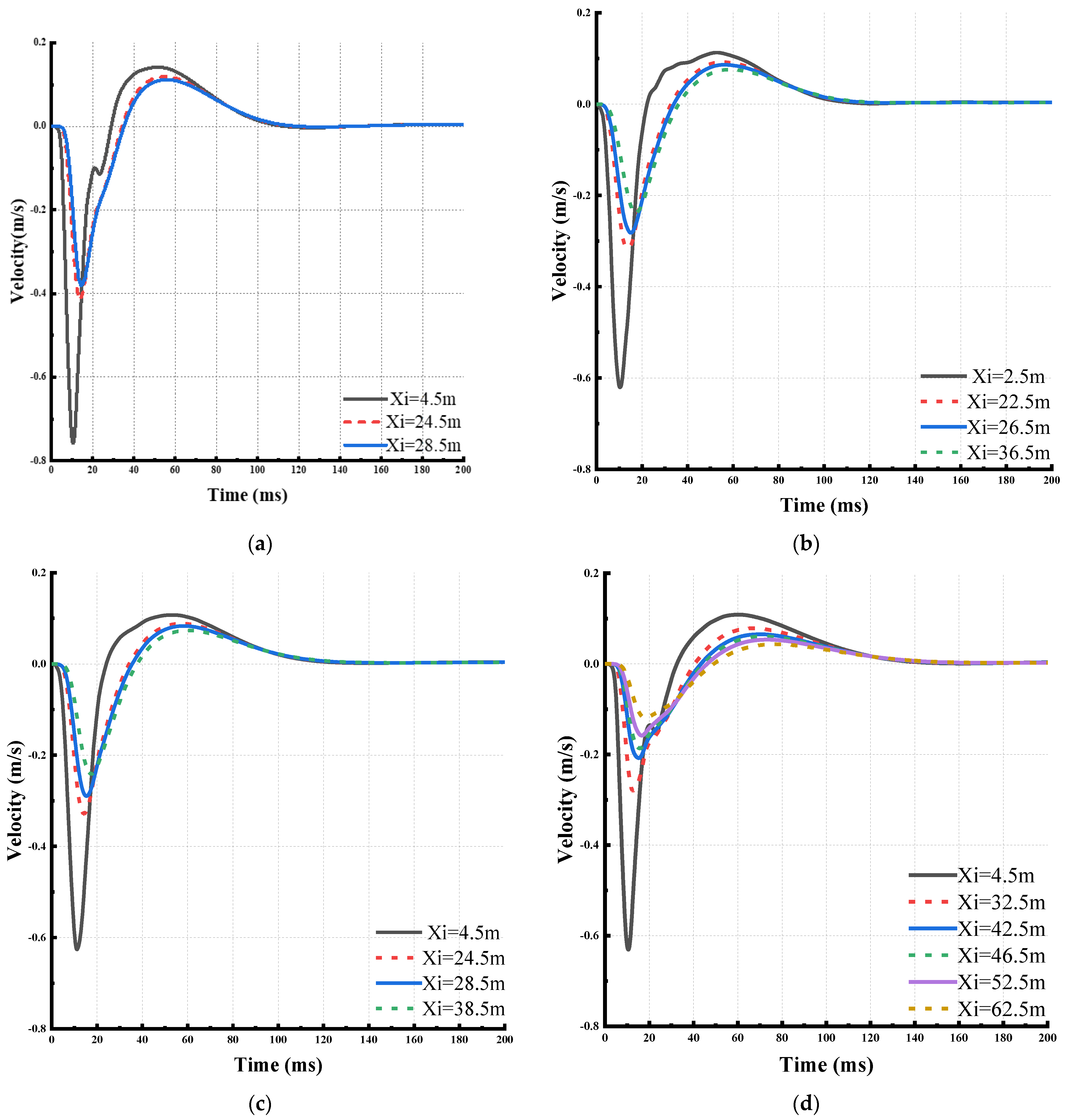
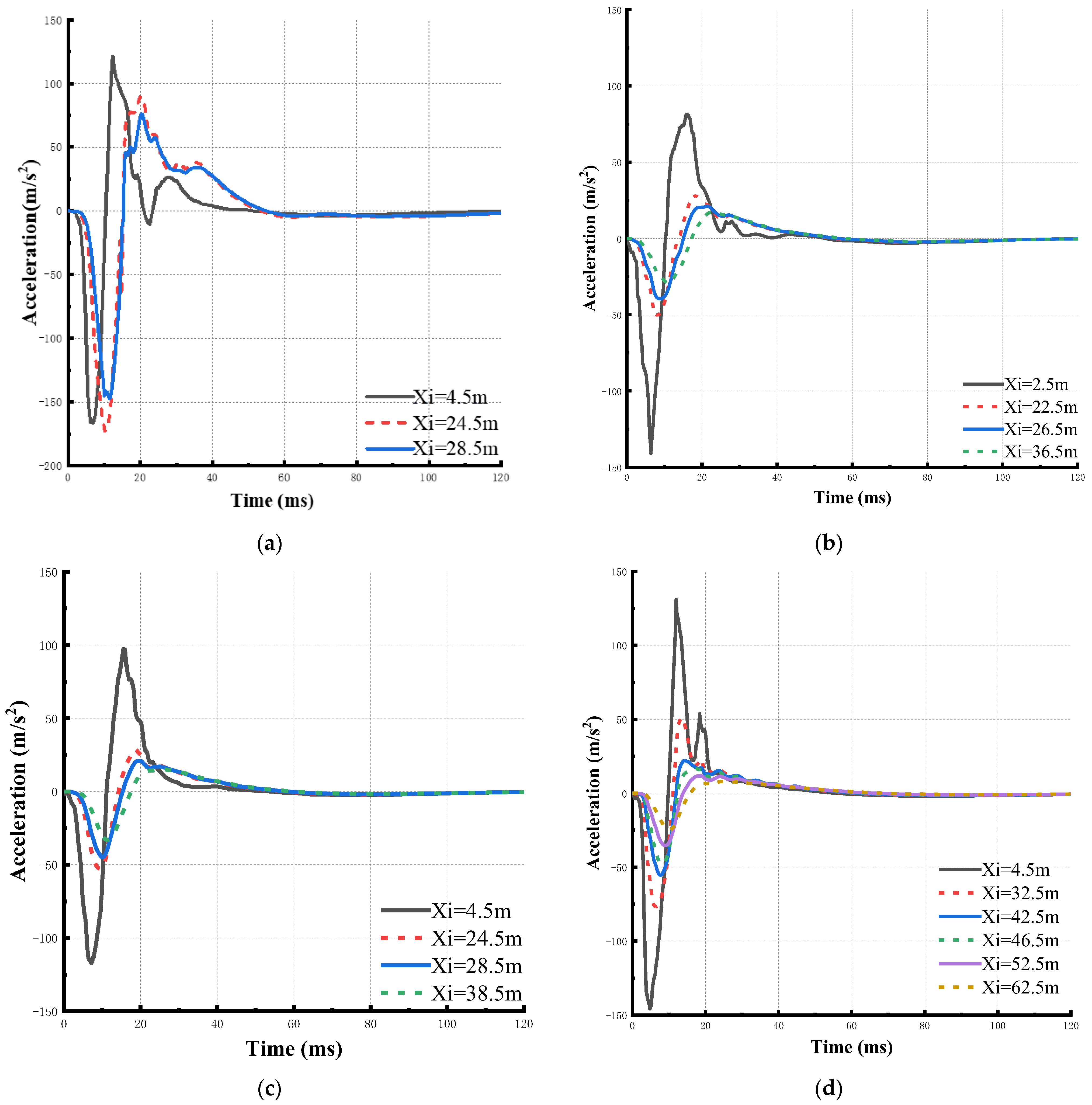
3.3. The High-Strain Direct Dynamic Test

After preparing the field test equipment, the pile hammer was lifted to the designated height and released from rest. Each hammer strike was followed by waiting for the pile to come to a complete stop before the next strike. The testing process strictly adhered to the provisions of the Code for Testing of Building Foundation (DBJ/T 15-60-2019) [39].

Using the high-strain dynamic tester and fiber optic demodulator, extensive strain and acceleration data were collected. A Python program was developed to process the input data, yielding time–history curves of velocity, acceleration, and dynamic resistance at various depths of the pile. The ultimate static side resistance for each pile segment was found through this analysis. These values were then added up to obtain the measured bearing capacity values for the four test piles, which can be seen in

Table 4. Measured value of test pile bearing capacity.

Pile No.	Maximum Impact Force at Pile Top (kN)	Pile Penetration (mm)	Pile Side Resistance (kN)	Vertical Designed Bearing Capacity of Single Pile (kN)	Vertical Allowable Bearing Capacity of Single Pile (kN)	Vertical Allowable Bearing Capacity of Single Pile (kN)
1–5	12,103.8	4.24	6637.7	4777.8	11,415.5	≥9510
2–7	10,907.1	2.13	6001.3	3732.0	9733.3	≥8688
3–9	11,540.5	3.44	7729.2	3059.2	10,788.4	≥9402
4–17	13,070.5	3.36	9012.7	3838.6	12,851.3	≥11,160

. The table also lists the single-blow penetration depths, as determined by the precision level. The table indicates that the single-blow penetration depths for all four test piles meet the code requirements (2–6 mm according to the local code), suggesting that the soil resistance around and below the piles was fully mobilized.

Given the soil layer distribution characteristics beneath arch bases 1–4, representative key measurement points were selected among the four test piles. At these points, Figure 7 and Figure 8 present the velocity and acceleration time–history curves, respectively. After the pile hammer’s significant impact force, the pile experienced downward acceleration, causing compressive deformation within the elastic range. As the impact force propagated downward, the velocity curves’ peak times varied at different depths, and the pile’s peak motion velocities gradually decreased. This reflects a reduction in axial force along the pile due to the side soil resistance. After the impact stopped, the pile rebounded elastically and eventually returned to a relatively static state.

By analyzing the axial forces at the upper and lower nodes of a pile segment and the segment’s average acceleration, the dynamic resistance of the segment at any time can be determined. Figure 9 illustrates the dynamic resistance time–history curve for a 2 m pile segment above a key node. As the relative displacement between the pile and soil increased, the soil resistance on the pile side also increased, leading to a gradual decrease in dynamic resistance and a corresponding reduction in the amplitude of its fluctuations. Eventually, the dynamic resistance reached a steady value rather than returning to zero because of the relative displacement between the pile and soil after the hammer impact. Since the hammer impact duration was very short, the surrounding soil did not undergo significant consolidation settlement, thus remaining relatively static. Therefore, side friction resistance continued to act after the pile’s self-vibration ceased.

Figure 10 shows the distribution of ultimate static resistance for each 2 m pile segment of the four test piles. It is important to note that the ultimate side resistance for each segment was achieved at different times. Some pile segments experienced tensile resistance, while others experienced compressive resistance, because the transient dynamic load’s short duration prevented drainage consolidation in the upper soft soil layers. During this phase, the pile moved downward relative to the soil, resulting in upward-side friction at the pile–soil interface. Consequently, the segments within the upper soft soil layers experienced tensile resistance. As the pile entered coarse sand layers and embedded into rock, its displacement was constrained by the rock layer at the pile base, resulting in compressive resistance. This analysis confirms that the high-strain dynamic testing method’s measured ultimate static side resistance aligns with the soil layer distribution beneath the four arch bases, verifying its feasibility in predicting single pile bearing capacity in engineering practice.

Considering that the pile primarily endures long-term static loads rather than instantaneous dynamic loads, the direction of static side friction resistance opposes the pile’s movement direction. Thus, summing the absolute values of each segment’s ultimate static resistance yields the pile’s overall ultimate static resistance.

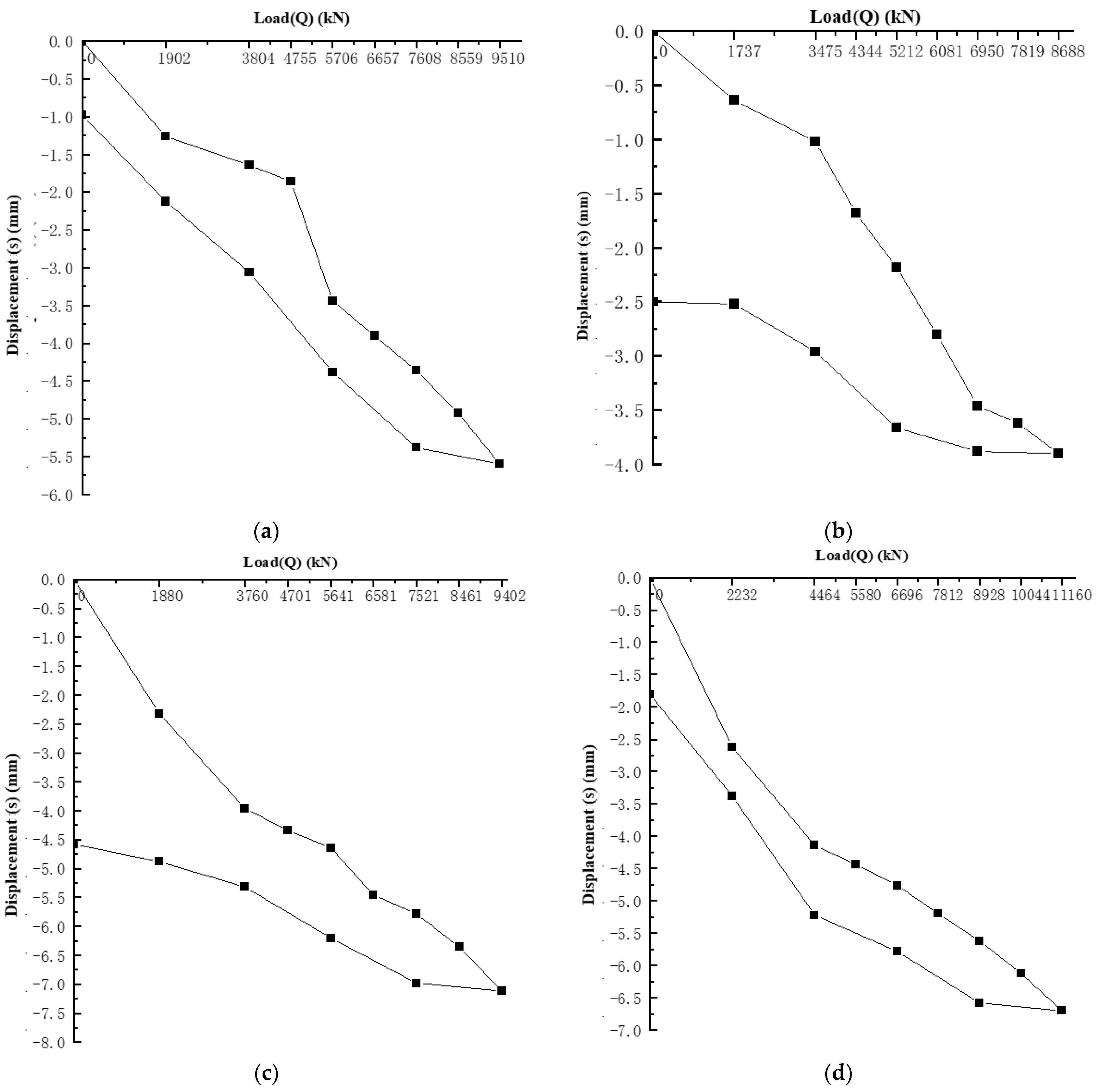
3.4. The Static Load Test

To avoid interference from dynamic load tests, static load tests were conducted after a 28-day resting period. The displacement of the four test piles under load over time was recorded in detail during the loading and unloading processes, resulting in the load–settlement (Q-s) curves shown in Figure 11. These curves indicate no sharp drops, suggesting no failure in the piles or bearing layers, thus meeting the expected safety and functional requirements.

The FBG sensors embedded within the piles continued to monitor strain distribution during loading, enabling the calculation of axial force distribution changes with increasing loads. Figure 12 shows the axial force distribution curves for the four test piles at load levels of 0.4, 1, and 2 times the characteristic bearing capacity.

The axial force initially increases with depth under negative friction before reaching a turning point and then decreases as depth increases because of the transition from negative to positive friction. This turning point, where pile settlement equals foundation settlement, is known as the “neutral point”. In Figure 11 and Figure 12, the highest axial force in the test piles is shown to be 11,005.7 kN, 10,096.0 kN, 10,946.6 kN, and 14,196.8 kN, respectively, at the highest test load. This force is higher than the designed ultimate bearing capacity. Despite these high forces, the piles did not fail, suggesting that the actual ultimate bearing capacity is more than twice the characteristic bearing capacity, thus making this conservative estimation reliable.

3.5. Comparison between the Results of the Dynamic Load Test and the Static Load Test

To evaluate the accuracy of high-strain testing using the static load test as a standard, three conditions must be considered. First, both dynamic and static load tests must be conducted on the same test pile and in the same soil conditions. Second, soil resistance must be fully mobilized. Third, the pile’s failure modes must be identical in both tests. The results of dynamic and static tests are comparable only if the pile fails to overcome soil resistance in both methods. The four test piles in this study meet these three conditions.

As previously mentioned, in regions with thick, soft clay, the actual maximum axial force on the pile during a static load test is greater than the designed ultimate bearing capacity because of negative skin friction. The high-strain method is typically used to predict the pile’s ultimate bearing capacity. To assess its accuracy, this study compares the actual maximum axial force measured during the static load test with the bearing capacity predicted by the high-strain dynamic test.

Table 5. Comparison between the results of the dynamic load test and the static load test.

Number (#)	Length (m)	Dynamic Load Test		Static Load Test
		Displacement (mm)	Ultimate Bearing Capacity (kN)	Displacement (mm)	Ultimate Bearing Capacity (KN)
1–5	34	4.24	11,415.5	5.60	11,005.7 (3.7%)
2–7	42.5	2.13	9733.3	3.90	10,096.0 (−3.6%)
3–9	48	3.44	10,788.4	7.12	10,946.6 (−1.4%)
4–17	68	3.36	12,851.3	6.70	14,196.8 (−9.5%)

presents the comparison results, showing that the error range between the high-strain method and the static load method is −9.5% to 3.7%. This indicates that the high-strain dynamic test is reliable for evaluating pile-bearing capacity. The main reason for the small error is that both tests determine the maximum load according to relevant standards, which ensures sufficient mobilization of soil resistance without damaging the pile material.

The following potential sources of error exist when using the high-strain dynamic method to predict the ultimate bearing capacity of piles:

(1)

Order of Testing: The dynamic load test was conducted before the static load test. Repeated hammering can densify the soil around the pile, potentially leading to an underestimation of the ultimate bearing capacity by the high-strain method and an overestimation by the static load method.

(2)

Sensor Placement: The segment of the pile near the bottom includes the side resistance up to the sensor $S{E}_N$. Therefore, the actual end-bearing resistance is less than the calculated value. For more accurate measurement, strain sensors should be placed closer to the actual pile tip.

(3)

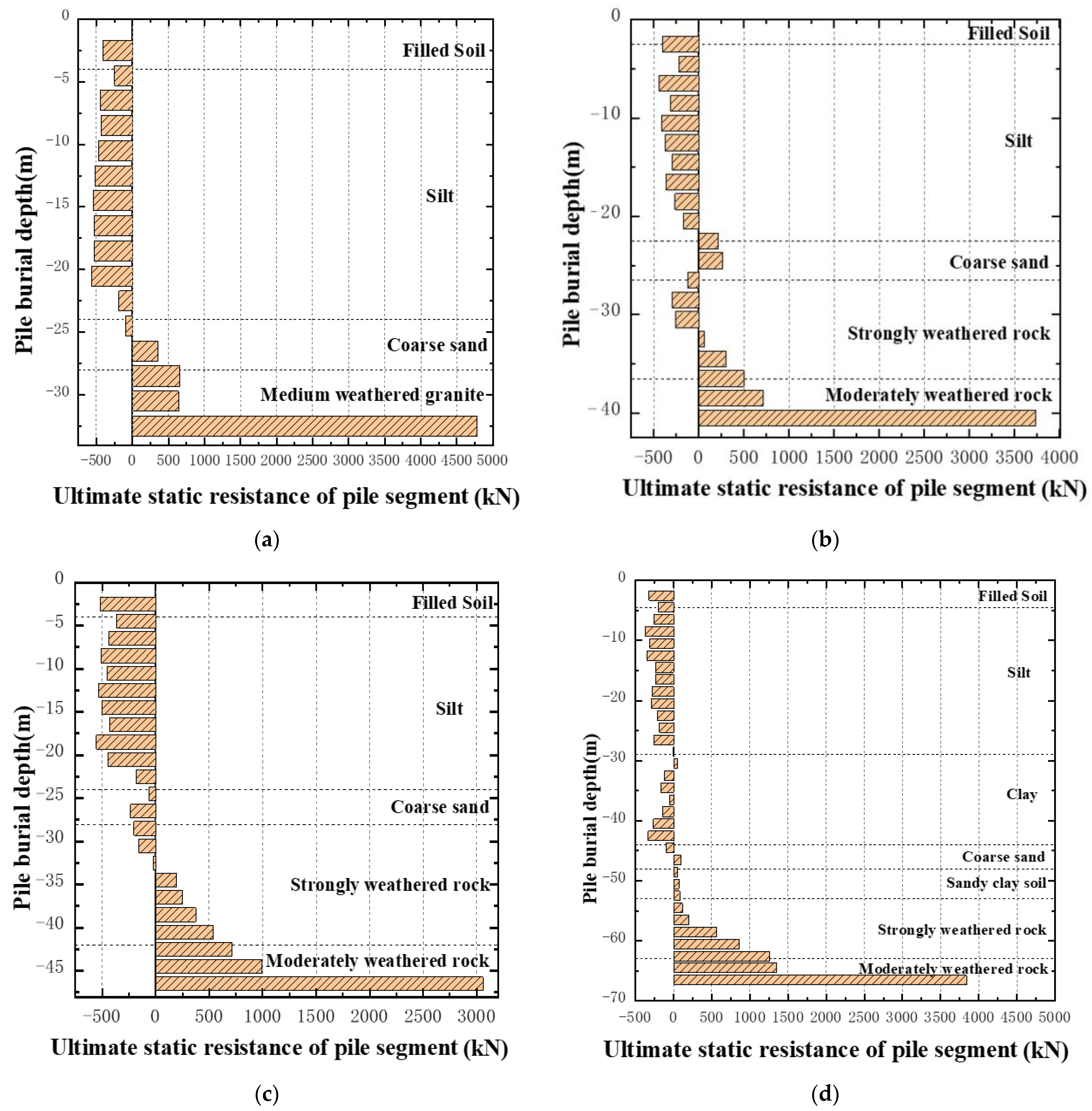
Boundary Effects: As observed in Figure 10, some pile segments located at the boundary between soft and hard soil layers exhibit lower ultimate static resistance compared with other segments. This is due to the change in the direction of forces on the pile side at these boundaries. When calculating dynamic resistance using Equation (10), opposing pressure and tension forces can cancel out, leading to lower resistance values. In practice, increasing the number of measurement points, reducing the spacing between them, and deploying a denser array of strain sensors at soil boundaries can enhance prediction accuracy.

By addressing these potential errors, the high-strain direct dynamic testing method can be more accurately applied to predict the ultimate bearing capacity of piles.

4. Conclusions

This paper focuses on the application study of a recently proposed dynamic testing method for pile-bearing capacity—the high-strain direct testing method. Using a bridge project in Zhuhai as the engineering background, field tests were conducted to verify the feasibility and reliability of this method in practical engineering applications. The main conclusions are as follows:

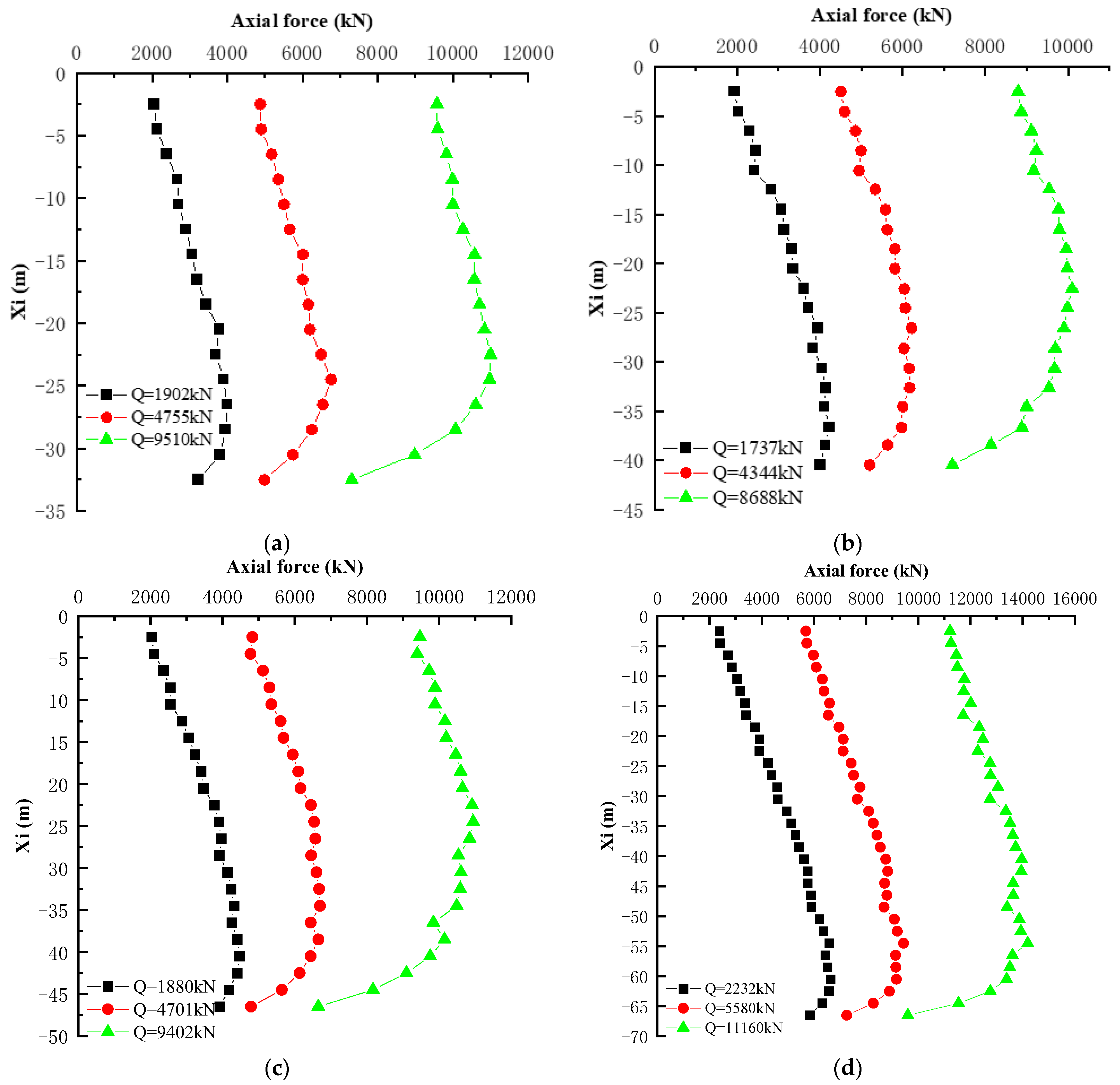
• The high-strain direct testing method was implemented in a bridge project in Zhuhai, Guangdong Province. The measured bearing capacities of four test piles were 11,415.5 kN, 9733.3 kN, 10,788.4 kN, and 12,851.3 kN, with end resistance ratios of 41.8%, 38.3%, 28.4%, and 31.8%, respectively, consistent with the bearing capacity characteristics of rock-socketed piles at the site. The calculated distributions of side and end soil resistance matched the soil layer distributions under the four arch bases, confirming the feasibility of the high-strain direct testing method in engineering applications.
• A static compression test was conducted on a single pile, and the results were compared with those from the high-strain direct testing method. The error range between the two methods was found to be between −9.5% and 3.7%, demonstrating the reliability of the high-strain direct testing method in predicting the bearing capacity of single piles and identifying the sources of error in its practical application.

Finally, the high-strain direct dynamic testing method calculates the bearing capacity of pile segments directly through the dynamic equilibrium equation, ensuring an accurate and unique ultimate bearing capacity for single piles, independent of the operator’s experience. This method provides a more precise description of the static soil resistance distribution along the pile shaft in various soil layers. The inferred soil parameters are more accurate, better reflecting the actual soil conditions on-site. Future researchers can integrate the field measurements obtained by this method with numerical simulation techniques to perform inverse analysis of the mechanical parameters of the soil surrounding the pile. This combined approach offers reliable data for engineering applications.

References

1. Qiu, H.; Zhou, Y.; Ayasrah, M.M. Impact study of deep foundations construction of inclined and straight combined support piles on adjacent pile foundations. Appl. Sci. 2023, 13, 1810. [Google Scholar] [CrossRef]
2. Qiu, H.; Wang, H.; Ayasrah, M.M.; Zhou, Z.; Li, B. Study on horizontal bearing capacity of pile group foundation composed of inclined and straight piles. Buildings 2023, 13, 690. [Google Scholar] [CrossRef]
3. Huang, W.; Liu, J.; Wang, H.; Ayasrah, M.M.; Qiu, H.; Wang, Z. Study on dynamic response of inclined pile group foundation under earthquake action. Buildings 2023, 13, 2416. [Google Scholar] [CrossRef]
4. Ayasrah, M.; Fattah, M.Y. Finite element analysis of two nearby interfering strip footings embedded in saturated cohesive soils. Civ. Eng. J. 2023, 9, 752–769. [Google Scholar] [CrossRef]
5. Issacs, D.V. Reinforced concrete pile formulas. Trans. Inst. Eng. 1993, 12, 305–323. [Google Scholar]
6. Smith, E.A.L. Pile driving analysis by the wave equation. American Society of Civil Engineers. ASCE J. Soil Mech. Found. Eng. 1960, 86, 35–61. [Google Scholar] [CrossRef]
7. Goble, G.G.; Scanlan, R.H.; Tomko, J.J. Dynamic Studies on the Bearing Capacity of Piles. In Proceedings of the Ohio Highway Engineering Conference Proceedings, Columbus, OH, USA, 2 May 1967. [Google Scholar]
8. Goble, G.G.; Rausche, F. Pile load test by impact driving. In Highway Research Record No. 333; Highway Research Board: Washington, DC, USA, 1970. [Google Scholar]
9. Goble, G.G.; Moses, F.R.E.D.; Rausche, F.R.A.N.K. Prediction of pile behavior from dynamic measurements. In Design and Installation of Pile Foundations and Cellular Structures; 1970. [Google Scholar]
10. Rausche, F. Soil Response from Dynamic Analysis and Measurements on Piles. Ph.D. Thesis, Case Western Reserve University, Cleveland, OH, USA, 1970. [Google Scholar]
11. Rausche, F.; Moses, F.; Goble, G.G. Soil Resistance Predictions from Pile Dynamics. J. Soil Mech. Found. Div. 1972, 98, 917–937. [Google Scholar] [CrossRef]
12. Goble, G.G.; Likins, G., Jr.; Rausche, F. Rausche Bearing Capacity of Piles from Dynamic Measurements. Ph.D. Thesis, Case Western Reserve University, Cleveland, OH, USA, 1975. [Google Scholar]
13. Goble, G.G. The analysis of pile driving-A state-of-the-art. In Proceedings of the International Conference on the Application of Stress-Wave Theory to Piles, Stockholm, Sweden, 4–5 June 1980. [Google Scholar]
14. Goble, G.G.; Rausche, F. Wave Equation Analysis of Pile Driving: WEAP Program; Final Rep. No. FHWA/IP-76-14.2; FHWA: Washington, DC, USA, 1976; Volume II. [Google Scholar]
15. Rausche, F.G.; Goble, J.G.; Likins, G.E., Jr. Dynamic Determination of Pile Capacity. J. Geotech. Eng. 1985, 111, 367–383. [Google Scholar] [CrossRef]
16. Holeyman, A.E. Dynamic non-linear skin friction of piles. In International Symposium on Penetrability and Driveability of Piles; Springer: San Francisco, CA, USA, 1985; Volume 1, pp. 173–176. Available online: https://www.fondytest.com/Alain-Holeyman-s-publications/pdf/1985-SF-Symposium-1.pdf (accessed on 1 July 2024).
17. Lee, S.; Chow, Y.; Karunaratne, G.; Wong, K. Rational wave equation model for pile-driving analysis. J. Geotech. Eng. 1988, 114, 306–325. [Google Scholar] [CrossRef]
18. Alwalan, M.F.; El Naggar, M.H. Analytical models of impact force-time response generated from high strain dynamic load test on driven and helical piles. Comput. Geotech. 2020, 128, 103834. [Google Scholar] [CrossRef]
19. Tu, Y.; El Naggar, M.H.; Wen, M.; Wang, K.; Wu, J. Dynamic analysis model of open-ended pipe piles that considers soil plug slippage. Comput. Geotech. 2023, 158, 105386. [Google Scholar] [CrossRef]
20. Deeks, A.J.; Randolph, M.F. A simple model for inelastic footing response to transient loading. Int. J. Numer. Anal. Methods GeoMech. 1995, 19, 307–329. [Google Scholar] [CrossRef]
21. Rausche, F.; Beth, R.; Garland, L. Multiple blow CAPWAP analysis of pile dynamic records. In Proceedings of the 5th International Conference on the Application of Stress-Wave Theory to Piles, Orlando, FL, USA, 11–13 September 1996; Volume 1, pp. 435–446. [Google Scholar]
22. Guin, J. Advanced Soil-Pile-Structure Interaction and Nonlinear Pile Behavior. Ph.D. Thesis, State University of New York at Buffalo, Buffalo, NY, USA, 1997. [Google Scholar]
23. Bruno, D.; Randolph, M.F. Dynamic and static load testing of model piles driven into dense sand. J. Geotech. Geoenviron. Eng. 1999, 125, 988–998. [Google Scholar] [CrossRef]
24. Kucukarslan, S. Linear and Nonlinear Soil–Pile–Structure Interaction under Static and Transient Impact Loading. Ph.D. Thesis, State University of New York at Buffalo, Buffalo, NY, USA, 2000. [Google Scholar]
25. Savvides, A.A.; Antoniou, A.A.; Papadopoulos, L.; Monia, A.; Kofina, K. An estimation of clayey-oriented rock mass material properties, sited in Koropi, Athens, Greece, through feed-forward neural networks. Geotechnics 2023, 3, 975–988. [Google Scholar] [CrossRef]
26. Chen, W.; Sarir, P.; Bui, X.-N.; Nguyen, H.; Tahir, M.M.; Armaghani, D.J. Neuro-genetic, neuro-imperialism and genetic programing models in predicting ultimate bearing capacity of pile. Eng. Comput. 2019, 36, 1101–1115. [Google Scholar] [CrossRef]
27. Duan, M.; Xiao, X. Enhancing soil pile-bearing capacity prediction in geotechnical engineering using optimized decision tree fusion. Multiscale Multidiscip. Model. Exp. Des. 2024, 7, 2861–2876. [Google Scholar] [CrossRef]
28. Yuan, J.; Zhu, G. Pile wave Analysis Program by Optimization Methods under Large Strain of Soil. Chin. J. Geotech. Eng. 1990, 12, 1–11. [Google Scholar]
29. Svinkin, M.R. Some uncertainties in high-strain dynamic pile testing. In Geotechnical Engineering for Transportation Projects; 2004; pp. 705–714. Available online: https://ascelibrary.org/doi/10.1061/40744%28154%2957 (accessed on 1 July 2024).
30. Svinkin, M.R. High-strain dynamic pile testing—Problems and pitfalls. J. Perform. Constr. Facil. 2010, 24, 99. [Google Scholar] [CrossRef]
31. Verbeek, G.; David, T.; Peter, M. The subjective element in dynamic load testing results. In Proceedings of the IFCEE 2015, San Antonio, TX, USA, 17–21 March 2015; pp. 2577–2583. [Google Scholar]
32. Zhu, G.; Zhang, J. A Method and Device for Dynamic Measurement of Foundation Pile Bearing Capacity. Patent CN108589805B, 28 September 2018. [Google Scholar]
33. Jiang, W.; Zhu, G.; Zhang, J. A direct high-strain method for the bearing capacity of single piles. Rock Soil Mech. 2020, 41, 3500–3508. [Google Scholar]
34. Tu, Y. Pile-Soil Interaction Model and Multi-Point Dynamic Testing Method Along the Pile Under High-Strain Conditions. Ph.D. Thesis, Zhejiang University, Hangzhou, China, 2022. [Google Scholar]
35. Du, Y.; Wang, J.; Lin, Y. Analysis and Discussion of Several Issues in Dynamic and Static Contrast Test. Geotechnical Engineering World: Hong Kong, China, 2005. [Google Scholar]
36. Tian, K.; Yang, L. Check Measurement for Allowable Pile Bearing Capacity of Bored Piles Combining High Strain Dynamic Test with Static Loading Test. J. Water. Resour. Archit. Eng. 2007, 2, 78–80. [Google Scholar]
37. Zhang, X. Contrastive analysis between high-strain dynamic test and static load test for large-diameter cast-in-place piles. Geotech. Investig. Surv. 2016, 44, 75–78. [Google Scholar]
38. Liu, C.; Tang, M.; Hu, H.; Chen, H.; Liu, C.; Hou, Z. Comparative study on vertical compressive bearing behavior of PHC pipe piles based on high strain method and static load method. Build. Struct. 2022, 52, 136–140. [Google Scholar]
39. DBJT 15-60-2019; Guangdong Provincial Department of Housing and Urban-Rural Development. Code for Testing of Building Foundation, 20 May 2019. Available online: https://www.webfree.net/download/3265 (accessed on 1 July 2024).
Figure 1. Arrangement of transducers on the pile.
Applsci 14 06714 g001
Figure 2. Schematic diagram of pile segment divisions.
Applsci 14 06714 g002
Figure 3. Pile segment force diagram.
Applsci 14 06714 g003
Figure 4. Soil layer profile.
Applsci 14 06714 g004
Figure 5. FBG optic layout diagram. (a) Cross-section. (b) Longitudinal section.
Applsci 14 06714 g005
Figure 6. On-site construction drawings. (a) Fabrication of steel cage and binding of FBG. (b) Pouring concrete.
Applsci 14 06714 g006
Figure 7. Velocity time–history curves for (a) #1–5, (b) #2–7, (c) #3–9, and (d) #4–17.
Applsci 14 06714 g007
Figure 8. Acceleration time–history curves for (a) #1–5, (b) #2–7, (c) #3–9, and (d) #4–17.
Applsci 14 06714 g008
Figure 9. Dynamic resistance time–history curves for (a) #1–5, (b) #2–7, (c) #3–9, and (d) #4–17.
Applsci 14 06714 g009
Figure 10. Pile static resistance distribution curves of the four test piles (a) #1–5, (b) #2–7, (c) #3–9, and (d) #4–17.
Applsci 14 06714 g010
Figure 11. Q-s curves of the four test piles (a) #1–5, (b) #2–7, (c) #3–9, and (d) #4–17.
Applsci 14 06714 g011
Figure 12. Axial force curves of the four test piles (a) #1–5, (b) #2–7, (c) #3–9, and (d) #4–17.
Applsci 14 06714 g012