Analyzing Regulatory Impacts on Household Natural Gas Consumption: The Case of the Western Region of Ukraine

Abstract

In this study, we analyzed the impact of government regulatory institutions on households’ natural gas use behavior and suggested that the conventional view of natural gas as a social utility is inappropriate. Pursuing this goal, we applied correlation analysis, regression analysis and the Granger causality test to assess the statistically significant impact of particular factors (environmental temperature, price and tariff on natural gas) on household gas consumption. Our study was based on the data on household gas consumption in 2019–2022. Ultimately, the lowest rate of influence was recorded by the Granger causality test (2.47%), compared to 6.88% in the test for the significance of the correlation coefficient and 9.23% in the t-test for the statistical significance of the regression coefficients. One has to note that the Granger causality test used in our study is considered the most sensitive model for analyzing economic data. Using statistical methods, we concluded that regulatory factors have a negligible impact on the volume of natural gas consumption by households. Our results suggest that the Ukrainian regulatory authorities should be cautious about using non-market mechanisms, such as price caps, in the energy sector.

1. Introduction

Despite decades of reforms in Ukraine’s energy sector, the natural gas market for household consumers is still in a “suspended state” under the influence of “manual control”. The state authorities set the price of natural gas and the tariff for its distribution, namely the Cabinet of Ministers of Ukraine and the National Commission for State Regulation of Energy and Public Utilities, respectively.

At the same time, it is widely believed that natural gas is a socially critical commodity [1], and its distribution is a social function, unlike electricity or any other type of utility, the pricing of which is more market-based and less politicized.

Under such circumstances, household spending on natural gas is unjustifiably low, particularly in the overall structure of expenditures on utilities. On the other hand, this causes significant sectoral imbalances and the need to subsidize non-market prices from the state budget.

PSO is a dominant government tool to control energy markets in the current legislative framework. PSO (Public Service Obligation) is an obligation imposed on an organization by law or a contract to provide public interest service.

In April 2024, the Government of Ukraine extended the PSO mechanism till August 2024. It fixed the price of natural gas for household consumers at UAH 7.96 per 1 cubic meter (until April 2025). The same price (UAH 7.96) was valid from May 2021 to April 2024; meanwhile, in the last three years, inflation reached 137.23% and the cost of electricity for household consumers increased by 157.14% [2,3]. The same case can be observed within the tariff on the distribution of natural gas set by an independent regulatory authority—the National Commission for State Regulation of Energy and Public Utilities. These tariffs have not been revised for more than three years and have long been out of line with the level of expenses of gas distribution companies.

It is important to note that these populist decisions of the Ukrainian government directly contradict the basic principles of the natural gas market, which were once laid down in the European energy legislation, which is still being implemented quite actively in Ukraine, and cause significant imbalances in the energy market, as well as require significant amounts of funding from the state budget. In particular, for 2023, according to the financial plan of Naftogaz of Ukraine, the required compensation from the state budget for implementing the PSO mechanism exceeds UAH 300 billion (equivalent to USD 7.5 billion).

At the same time, the recently published report by the Energy Community “Ukraine Energy Market Observatory” was entitled “A need for the reforms of Ukraine’s gas market”—after the previous long period of implementation of the EU legislative codes in the energy sector was finally recognized as successful only two years earlier [4].

In particular, the Energy Community Secretariat recommends that Ukraine immediately start thinking about implementing reform processes based on the fundamental principles of the natural gas market that existed before the full-scale war on Ukraine’s territory while paying due attention to protecting the most vulnerable groups of the population [5,6].

Thus, the following questions are rightly on the agenda today: Is the perception of natural gas as a socially critical commodity, correct? How exactly do household consumers react to changes in prices and tariffs? Is it critical enough? What is the impact of regulatory factors on households’ natural gas consumption?

2. Literature Review

Various studies emphasize the significance of regulatory measures in shaping household energy consumption, particularly natural gas [7,8,9,10]. In Western Ukraine, these aspects are crucial due to the geopolitical situation and energy dependency on external suppliers [11,12].

A significant contribution to understanding the problems and prospects for the development of regional gas distribution markets was made by so many researchers [13,14,15,16]. Their works provide a thorough understanding of the theoretical foundations of the functioning of these markets, as well as the practical aspects of their activities.

A separate mention should be made of the works [17,18,19,20], which study innovative issues of the development of gas distribution companies to increase their competitiveness. Their research provides valuable information on how gas distribution companies can adapt to changing market conditions and remain competitive.

One critical indicator of gas distribution companies’ competitiveness is their market share [21]. A higher market share usually indicates a more stable position of the company and its ability to meet consumers’ needs [22].

Recent studies have expanded the focus to include the economic and social implications of natural gas dependency, highlighting the broader context in which regulatory factors operate. For instance, Kröger et al. (2022) examined the costs of natural gas dependency, focusing on price shocks, inequality, and public policy [23]. This research is pivotal in understanding the socio-economic impacts of regulatory decisions in the energy sector. Similarly, Smajla et al. (2023) provided insights into short-term forecasting of natural gas consumption by determining the statistical distribution of consumption data [24], offering valuable methodologies for anticipating market responses to regulatory changes. Hooijmans (2016) explored the non-linear relation between natural gas consumption and temperature [25], and Wang et al. (2018) identified the correlation between ambient temperature and gas consumption in a local energy system [26]. These studies underscore the significance of environmental factors in gas consumption patterns, which interact with regulatory influences to shape overall consumption dynamics.

It is worth noting that many scholars [16,27,28,29] need to pay more attention to determining the level of influence of regulatory factors on household natural gas consumption. This aspect of the study is essential since the state’s regulatory policy can significantly affect consumer behavior and demand for natural gas.

Given the above, it was decided to investigate the impact of regulatory factors on households’ natural gas consumption in the western region of Ukraine. This research will provide valuable information on how regulatory policy affects consumer behavior and demand for natural gas and make recommendations for its improvement.

Studying the problems of the functioning and development of regional gas distribution markets is a relevant and promising area of scientific research. The works of domestic and foreign scholars make a significant contribution to understanding these problems and provide valuable information for developing practical recommendations for their solutions.

3. Aim of the Research

This paper investigates the impact of regulatory factors on the potential consumption of natural gas by households (retail consumers) in the western region of Ukraine. This study is conducted against the backdrop of years of reforms in the Ukrainian energy sector, which have yet to lead to the development of a natural gas market for household consumers. This market is still under strict state control, as the authorities set gas prices and distribution tariffs. Meanwhile, the tariffs are declared as being set according to the “cost plus” principle, and the price is determined arbitrarily with regard to “social justice”.

It is important to note that natural gas is traditionally considered a socially important commodity, and its distribution is a social function. This differs from electricity and other utilities, where pricing is more market-based and less dependent on political decisions. This study aims to determine how state regulation policy affects potential gas consumption by households.

4. Research Methodology

The purpose of this article is to study the influence of regulatory factors on the volume of natural gas consumption by household consumers, that is, to determine whether regulatory factors are statistically significant or not.

Regulatory factors—the decision of the «National Commission for State Regulation of Energy and Public Utilities» on setting tariffs for the distribution of natural gas, the decision of the Cabinet of Ministers on setting the price of natural gas for domestic consumers.

The primary data we used for research are as follows:

• Billing data—actual data of household consumers with a monthly breakdown and metadata (category of consumers, location, presence and type of gas meter, volume of consumption, etc.)
• Meteorological data—average monthly air temperature per month in Volyn region ([30], “Temperature.csv”)
• Actual prices of natural gas and tariffs for the distribution per cubic meter in relevant periods ([30], “Cost.csv”).

To perform research, 10% of Volyn region consumers data (n = 22,774, where n is the sample size) on monthly gas consumption in the period of June 2019–December 2022 were selected ([30], “Data.csv”). The selection was carried out using the method of stratified simple random sampling.

Thus, the following are variables used in our research:

• The volume of gas consumption per month (Consumption) in cubic meters (m³).
• The average monthly temperature (Temperature) in degrees Celsius (°C).
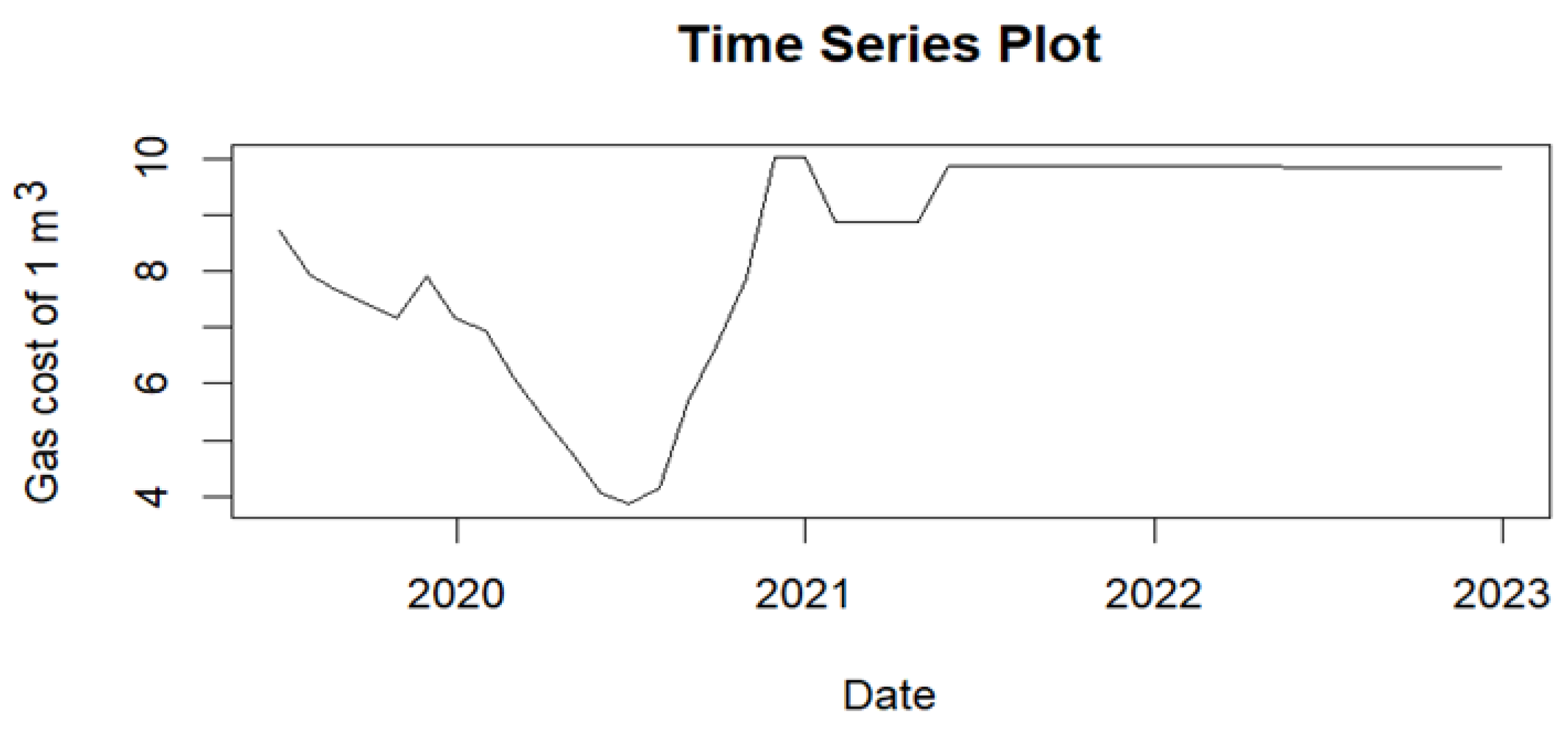
• The natural gas cost of 1 m³ (Cost) in UAH.

Using stratified simple random sampling without replacement we have divided the population into distinct strata (category of consumer) based on metadata and then performed simple random sampling within each stratum. This ensures that each category of consumers is represented in the sample.

Belonging to a certain category of consumers due to demands of the Ukrainian legislation and GTS Code [31] is defined by annual volume of consumption, type of building, type and quantity of appliances connected and living floor area. The category depicts the social status of the consumer and can be considered as a significant feature because it additionally allows for the measurement of the sensitivity of different social groups to regulatory effects.

Taking into account the specifics of the data (e.g., time series, seasonals, etc.), we will use correlation analysis, regression analysis and the Granger causality test as the most common research tools. In particular, the research methods we apply are as follows:

−

t-test statistical significance of the coefficients of regression [32,33,34];

−

Test for the significance of the correlation coefficient [32,35];

−

Granger causality test [33,36,37].

These methods will help us to understand how changes in gas prices and average temperature affect the volume of natural gas consumption by domestic consumers.

All the aforementioned models were applied to the sample data separately for each consumer and thereafter the results were summarized in a table in the section on separate categories of consumers.

The data analysis was built using R version 4.1.2. The working dataset and programming code are committed on GitHub [30].

5. Discussion

5.1. t-Test Statistical Significance of the Coefficients of Regression

In regression analysis, the t-test is commonly used to assess the statistical significance of individual regression coefficients. This test helps determine whether the independent variables (e.g., gas prices) have a statistically significant effect on the dependent variable (e.g., gas consumption).

Let us consider the following regression model:

$$y={\beta }_0+{\beta }_1{x}_1+{\beta }_2{x}_2+\epsilon ,$$

(1)

where $x_1$ is “the natural gas cost of 1 ${\mathrm{m}}^3$” (defined as a sum of price and tariff on distribution), $x_2$ is “the average monthly temperature”, $y$ is dependent/response variable that denotes “the volume of gas consumption per month”, ${\beta }_0$ is $y$-intercept (constant term), ${\beta }_1,{\beta }_2$ are slope coefficients for each independent/predictor variable and $\epsilon$ is the model’s error term.

Whenever we perform linear regression, we want to know if there is a statistically significant relationship between the independent/predictor variable and the dependent/response variable. We test for the significance of coefficients in the regression model by performing a t-test for the regression slope. We use the following null and alternative hypotheses for this t-test:

Null hypothesis $H_0: {\beta }_1=0$.

Alternative hypothesis $H_A: {\beta }_1\ne 0$.

The null hypothesis states that there is no relationship between the predictor variable and the response variable.

The test statistic is as follows:

$$t={\displaystyle \frac{{\widehat{\beta }}_1}{{\sigma }_{{\widehat{\beta }}_1}}},$$

(2)

where ${\sigma }_{{\widehat{\beta }}_1}$ is the standard error of ${\widehat{\beta }}_1$.

The relevant distribution is the $t$-distribution, with degrees of freedom $n-\left(k+1\right)$, where $k$ is the number of explanatory/predictor variables.

Using the calculated t-statistic and the degrees of freedom, we can find the p-value from the t-distribution. The p-value indicates the probability of observing a t-statistic as extreme as, or more extreme than, the one calculated if the null hypothesis is true.

Compare the p-value to chosen significance level α. If the p-value is less than α, we reject the null hypothesis and conclude that the coefficient is statistically significant.

Let us consider the following data for a single consumer (

Table 1. Monthly household natural gas consumption in 2019–2022 (source: authors’ development).

Time Period	Consumption, m3	Temperature, °C	Gas Cost of 1 m3, UAH
2019-06	18	21.7	8.732320
2019-07	24	18.9	7.935010
2019-08	28	19.8	7.624890
2019-09	24	14.7	7.428200
2019-10	33	10.9	7.156520
2019-11	80	6.3	7.926800
2019-12	103	2.6	7.161360
2020-01	99	1.3	6.960492
2020-02	105	2.9	6.097030
2020-03	81	4.7	5.418070
2020-04	33	8.5	4.804300
2020-05	27	11.7	4.040130
2020-06	21	19.6	3.876000
2020-07	24	19.2	4.150950
2020-08	25	19.7	5.675990
2020-09	23	15.3	6.675998
2020-10	37	11.1	7.876260
2020-11	73	5.0	10.012050
2020-12	104	1.4	10.012050
2021-01	115	−2.1	8.874000
2021-02	107	−3.6	8.874000
2021-03	10	2.5	8.874000
2021-04	147	6.8	8.874000
2021-05	21	13.1	9.874000
2021-06	19	19.8	9.874000
2021-07	28	22.7	9.874000
2021-08	27	17.5	9.874000
2021-09	1	12.3	9.874000
2021-10	87	8.2	9.874000
2021-11	90	4.6	9.874000
2021-12	115	−1.7	9.874000
2022-01	115	−0.8	9.874000
2022-02	108	1.4	9.874000
2022-03	82	2.4	9.874000
2022-04	57	5.7	9.874000
2022-05	39	12.1	9.844000
2022-06	10	18.0	9.840900
2022-07	1	18.3	9.840900
2022-08	8	19.9	9.840900
2022-09	5	11.1	9.840900
2022-10	48	10.0	9.840900
2022-11	81	3.5	9.840900
2022-12	64	−0.8	9.840900

) and apply the model described above.

Applying the t-test statistical significance of the coefficients of regression to the mentioned dataset in R [38], we obtain the following results (Figure 1 and Figure 2).

Interpreting Key Parameters:

Coefficients Estimate: provides the estimates for the intercept and slope of the regression line.

Std. Error: the standard error of the coefficient estimates.

t-value: the t-statistic for testing the null hypothesis that the coefficient is equal to zero.

$Pr(>\left|t\right|)$: the p-value associated with the t-statistic.

Residual standard error: an estimate of the standard deviation of the model residuals.

Multiple R-squared and Adjusted R-squared: measures of how well the model explains the variance in the dependent variable.

F-statistic: a statistic for testing the overall significance of the model.

We decide on the significance level $\alpha =0.05$. Here, a t-value of ${\beta }_1$ equals −0.239, $p-\mathrm{v}\mathrm{a}\mathrm{l}\mathrm{u}\mathrm{e}$= 0.812 and $p-\mathrm{v}\mathrm{a}\mathrm{l}\mathrm{u}\mathrm{e}>\alpha ,$ indicating that the coefficient is not statistically significant. This means there is sufficient evidence to suggest that the coefficient ${\beta }_1$ equals zero. The null hypothesis thus cannot be rejected.

Using the described model to the data of each consumer, we found there is no relationship between the predictor variable (“the natural gas cost of 1 ${\mathrm{m}}^3$”) and the response variable (“the volume of gas consumption per month”) in 90.77% of cases (20,673 cases above and equal and 2101 cases under the significance level respectively).

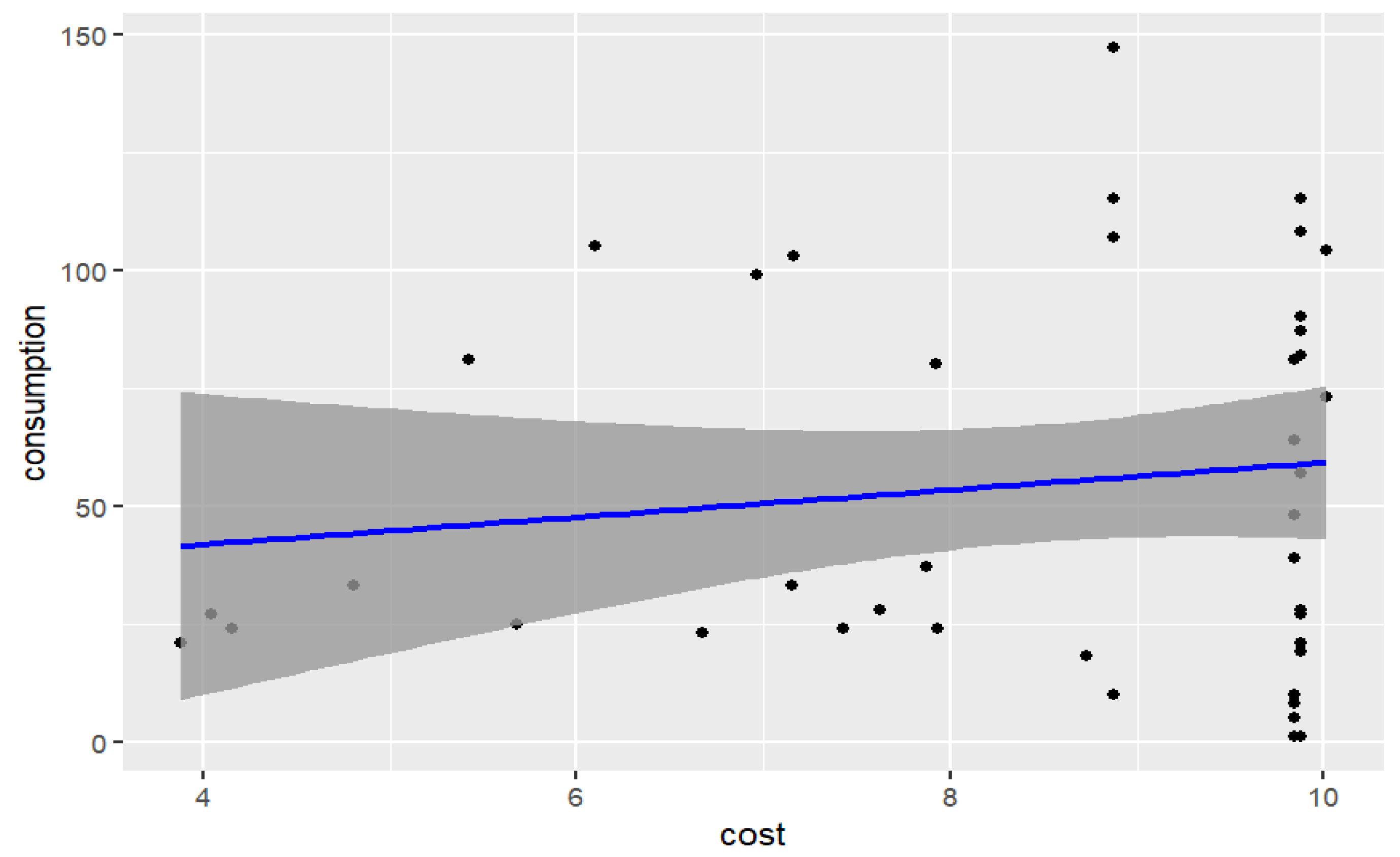
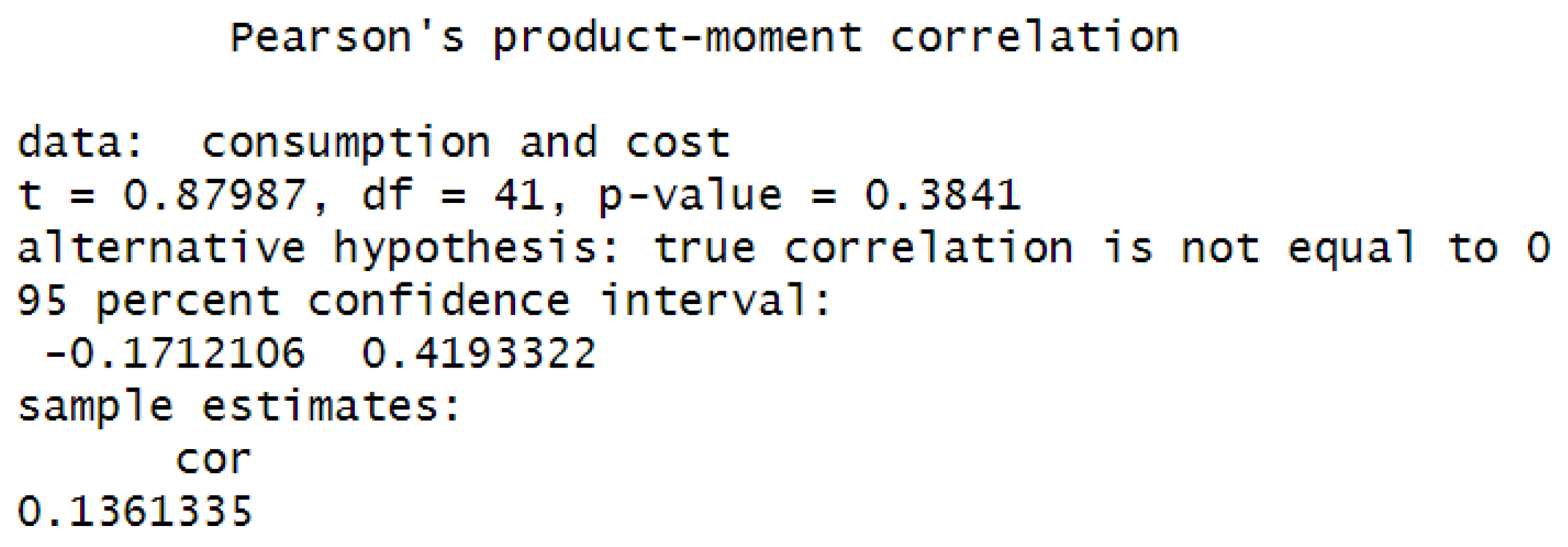
5.2. Test for the Significance of the Correlation Coefficient

The most common test for studying the significance of the correlation coefficient between two variables is the Pearson’s correlation coefficient test, which assumes that the data follow a bivariate normal distribution. Testing the significance of the correlation coefficient involves determining whether the observed correlation between two variables is statistically different from zero.

To determine whether a given Pearson’s correlation coefficient has a statistically significant result or not, we consider the next hypotheses:

Null hypothesis $H_0: \rho =0$ (there is no correlation between the two variables); where $\rho$ is the correlation coefficient.

Alternative hypothesis $H_A: \rho \ne 0$ (there is a significant correlation between the two variables).

The test statistic is as follows:

$$t={\displaystyle \frac{r_{xy}\sqrt{n-2}}{\sqrt{1-r_{xy}^2}}},$$

(3)

where $r_{xy}$ is the sample Pearson’s correlation coefficient, $r_{xy}={\displaystyle \frac{{\sum }_{i=1}^n(x_i-\overline{x})(y_i-\overline{y})}{\sqrt{{\sum }_{i=1}^n{(x_i-\overline{x})}^2{(y_i-\overline{y})}^2}}}$, $x_i$ is $x$ variable samples, $y_i$ is $y$ variable samples, $\overline{x}$ is mean of values in $x$ variable and $\overline{y}$ is mean of values in $y$ variable.

Relevant distribution is the $t$-distribution, with degrees of freedom $n-2$.

Using the calculated t-statistic and the degrees of freedom, we can find the p-value from the t-distribution. The p-value indicates the probability of observing a t-statistic as extreme as, or more extreme than, the one calculated if the null hypothesis is true.

We compare the p-value to the chosen significance level α. If the p-value is less than α, we reject the null hypothesis and conclude that the correlation coefficient is statistically significant.

Let us test the significance of Pearson’s correlation coefficient between “the volume of gas consumption per month” for a single consumer and “the natural gas cost of 1 ${\mathrm{m}}^3$”. The level of significance chosen is α = 0.05. Using the data (Table 1), we obtain the following results (Figure 3 and Figure 4).

Interpreting Key Parameters:

Pearson’s correlation coefficient (cor): the sample correlation coefficient between $x$ and $y$.

Test statistic ($t$): the t-statistic for testing the null hypothesis that the true correlation coefficient is zero.

Degrees of freedom (df): the degrees of freedom associated with the t-statistic.

p-value: the p-value for the test.

Confidence interval: a confidence interval for the true correlation coefficient.

Since $p-\mathrm{v}\mathrm{a}\mathrm{l}\mathrm{u}\mathrm{e}=0.3841$ and $p-\mathrm{v}\mathrm{a}\mathrm{l}\mathrm{u}\mathrm{e}>\alpha$, therefore the null hypothesis cannot be rejected, and we conclude that the correlation between “the volume of gas consumption per month” for a single consumer and “the natural gas cost of 1 ${\mathrm{m}}^3$” is not statistically significant.

Applying the described above model to the data of each consumer, we have determined that there is no relationship between “the natural gas cost of 1 ${\mathrm{m}}^3$” and “the volume of gas consumption per month” in 93.12% of cases (21,208 cases above and equal, and 1566 cases under the significance level, respectively).

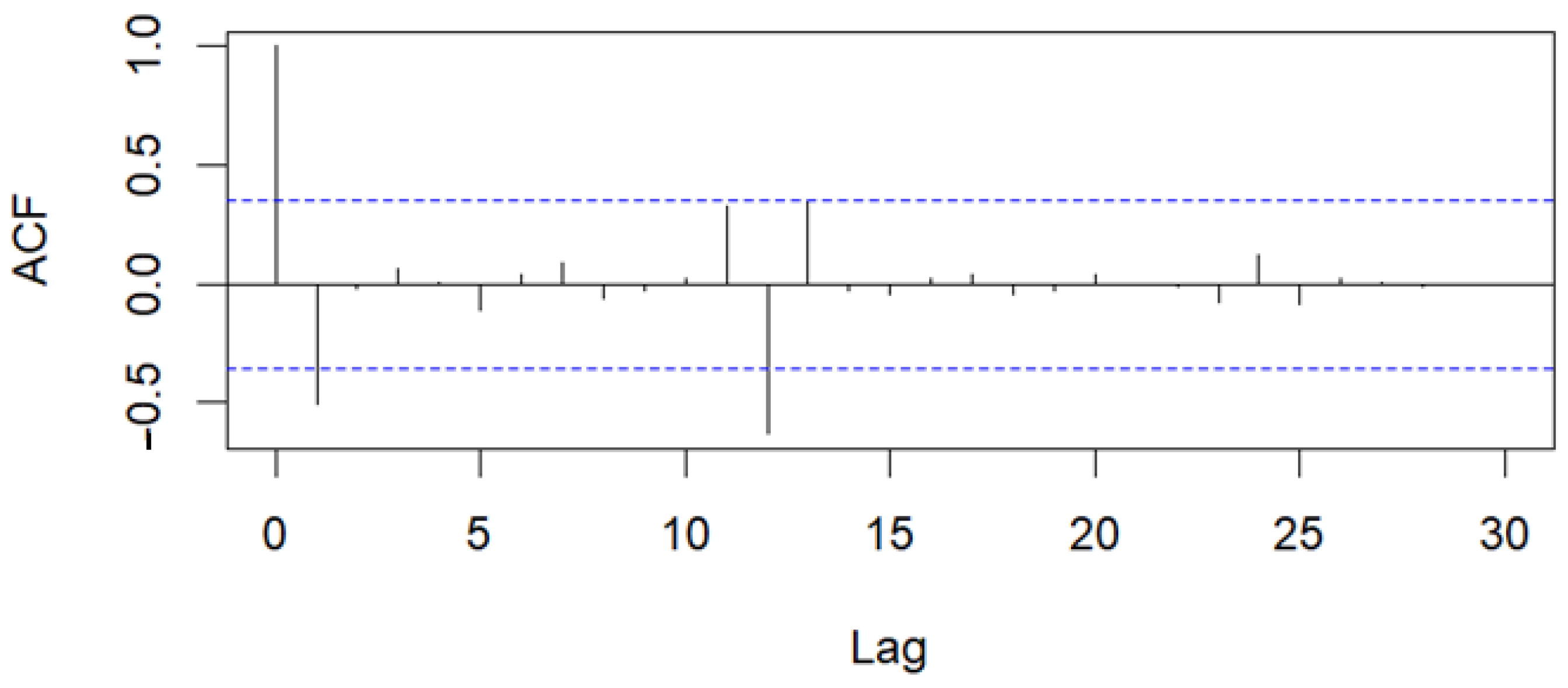
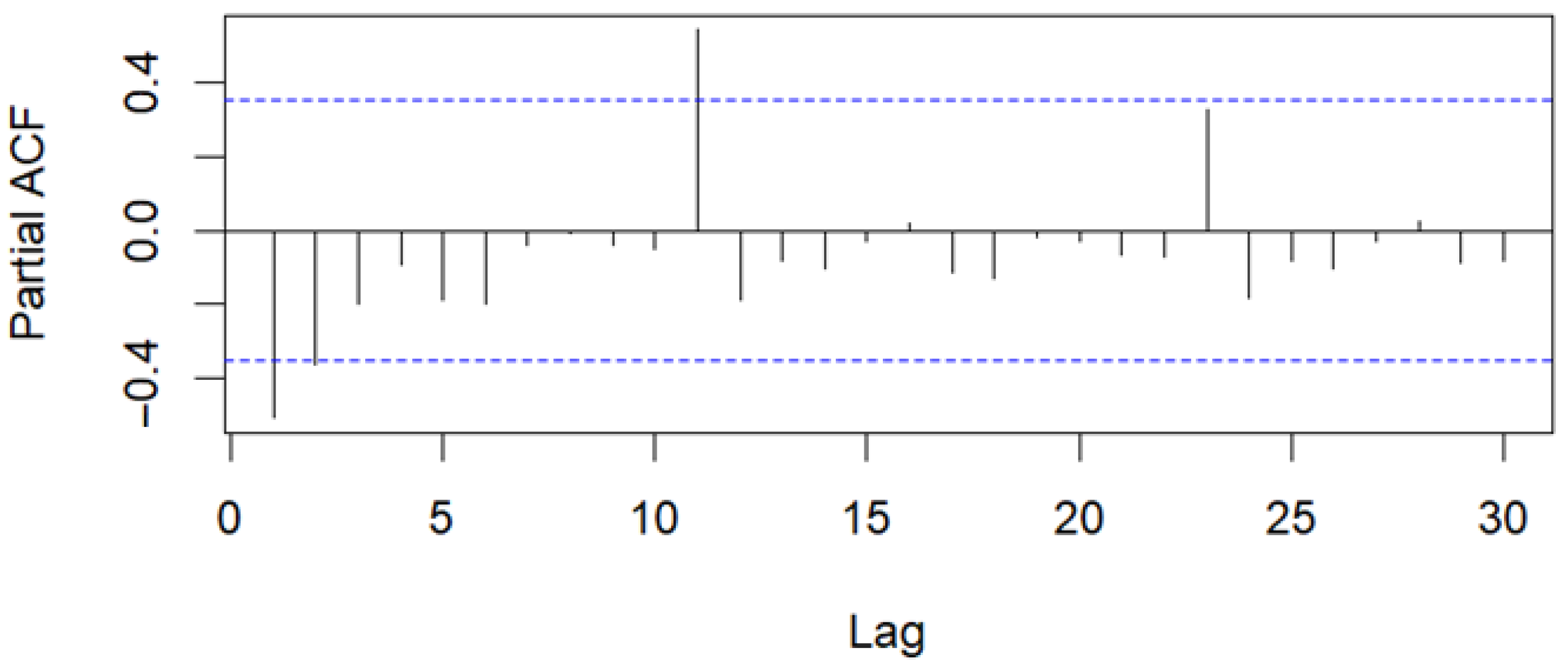
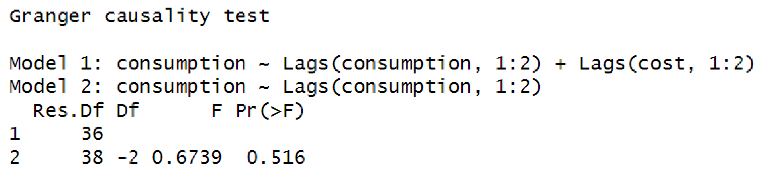
5.3. Granger Causality Test

Granger causality test [36] is a statistical hypothesis test to determine whether one time series can be used to predict another. It assesses whether past values of one variable can provide information about the future values of another variable, thus indicating a directional influence. The test is based on the idea that if variable $X$ Granger causes variable $Y$, then past values of $X$ should contain information that helps predict $Y$.

Let us consider the case of testing whether time series $X$ Granger causes time series $Y$. The models can be formulated as follows:

• Unrestricted model (URM):

URM includes both the lagged values of $X$ and $Y$ to predict $Y$.

$$Y_t=\alpha +{\beta }_1{Y}_{t-1}+{\beta }_2{Y}_{t-2}+\cdots +{\beta }_p{Y}_{t-p}+{\gamma }_1{X}_{t-1}+{\gamma }_2{X}_{t-2}+\dots +{\gamma }_q{X}_{t-q}+{\epsilon }_t.$$

(4)

2.

Restricted model (RM):

RM includes only the lagged values of $Y$ to predict $Y$, excluding the lagged values of $X$.

$$Y_t=\alpha +{\beta }_1{Y}_{t-1}+{\beta }_2{Y}_{t-2}+\cdots +{\beta }_p{Y}_{t-p}+{\epsilon }_t,$$

(5)

The time series $X$ and $Y$ must be stationary (mean and variance are constant over time). This can be performed using unit root tests like the Augmented Dickey–Fuller (ADF) test. If the data are not stationary, then they needs to be transformed (e.g., differenced) until stationarity is achieved.

We say $X$ does not Granger cause $Y$ if the following is true:

$$E\left(Y_t\left|Y_{t-1},Y_{t-2},\dots ,Y_{t-p},X_{t-1},X_{t-2}\dots ,X_{t-q}\right.\right)=E\left(Y_t\left|Y_{t-1},Y_{t-2},\dots ,Y_{t-p}\right.\right).$$

Thus, the null hypothesis $H_0$ for the Granger causality test is that past values of $X$ do not Granger-cause $Y$. This hypothesis implies that the coefficients ${\gamma }_1, {\gamma }_2,\dots ,{\gamma }_q$ of the lagged values of $X$ in the URM are jointly equal to zero ($H_0: {\gamma }_1={\gamma }_2=\cdots ={\gamma }_q=0$). Alternative hypothesis $H_A$: at least one ${\gamma }_i\ne 0$.

The test statistic is based on the comparison of the sum of squared residuals (SSR) from the unrestricted and restricted models. The F-statistic is then calculated as follows:

$$F={\displaystyle \frac{\frac{{SSR}_{RM}-{SSR}_{URM}}{q}}{\frac{{SSR}_{URM}}{T-p-q-1}}},$$

(6)

where ${SSR}_{RM}$ is the sum of squared residuals from the restricted model; ${SSR}_{URM}$ is the sum of squared residuals from the unrestricted model; $T$ is the number of observations; $p$ is the number of lags in the model (order of autoregression for $Y$); $q$ is the number of lags in the model (order of autoregression for $X$).

To select the number of lags $(p, q)$ included in models (4) and (5), we will apply a graphical analysis of the autocorrelation function of time series (ACF shows the relationship between the values of the time series at different moments in time) and the partial autocorrelation function of time series (PACF shows the relationship between the values of the time series at different moments of time, excluding the influence of other lags), and also the Akaike Information Criterion (AIC) or the Schwarz criterion (SC), also known as the Bayesian Information Criterion (BIC).

The F-statistic follows an F-distribution with degrees of freedom $q$ in the numerator and $T-p-q-1$ in the denominator. If the F-statistic is significant at a chosen significance level, the null hypothesis is rejected, indicating that past values of X Granger-cause Y.

Denote the variable $Y$ is the volume of gas consumption per month, the variable $X$ is the natural gas cost of 1 ${\mathrm{m}}^3$. Let us check whether time series $X$ Granger causes time series $Y$ using the Granger causality test [39].

At first, we draw the basic time series plots (Figure 5 and Figure 6) of “the natural gas cost of 1 ${\mathrm{m}}^3$” and “the volume of gas consumption per month” for a single consumer of data mentioned above (Table 1) to analyze their relationship and identify seasonal fluctuations and long-term trends.

Analyzing the time series plots shown above, we do not see a cause-and-effect relationship between two variables (“the volume of gas consumption per month” and “the natural gas cost of 1 ${\mathrm{m}}^3$”) visually. Therefore, we will use the Granger causality test to investigate the cause-and-effect relationship between the specified variables.

First, let us determine the lag order for the Granger causality test. To do this, we will perform a graphical analysis of the ACF and PACF for "the natural gas cost of 1 ${\mathrm{m}}^3$”, and "the volume of gas consumption per month," as well as use the AIC and SC criteria.

The time series of “the natural gas cost of 1 ${\mathrm{m}}^3$” is not stationary. By applying two different transformations, we convert the time series of “the natural gas cost of 1 ${\mathrm{m}}^3$” into a stationary time series.

Since the time series of “the volume of gas consumption per month” has the property of seasonality, we decompose it into its seasonal, trend and residual components using techniques like the Seasonal Decomposition of Time Series, and analyze the remaining part to determine the appropriate lag order.

Let us plot the autocorrelation function (ACF) and partial autocorrelation function (PACF) of the new stationary time series of “the natural gas cost of 1 ${\mathrm{m}}^3$” (Figure 7 and Figure 8) of the residual component of the time series of “the volume of gas consumption per month” (Figure 9 and Figure 10) and look for significant lags beyond which autocorrelation becomes negligible. The number of lags at which the ACF and PACF drop to zero or become insignificant can provide a visual indication of the lag order.

Taking into account Figure 7, Figure 8, Figure 9 and Figure 10 and the results of AIC and SC (the model with the smallest AIC, or the smallest SC, is preferred), we concluded that the order lags take the values $\left(p, q\right)=(2, 2)$.

Let us check the null hypothesis of the Granger causality test for a single consumer of data (Table 1). We obtain the next result (Figure 11).

Interpreting Key Parameters:

F-statistic: the test statistic for the Granger causality test.

p-value: the p-value associated with the F-statistic.

Degrees of freedom (df): the degrees of freedom associated with the F-statistic.

The chosen level of significance is $\alpha =0.05$. Since $p-\mathrm{v}\mathrm{a}\mathrm{l}\mathrm{u}\mathrm{e}=0.516$, $p-\mathrm{v}\mathrm{a}\mathrm{l}\mathrm{u}\mathrm{e}>\alpha$, therefore the null hypothesis cannot be rejected. This This means that past values of variable X (“the natural gas cost of 1 m³”) do not indicate that X Granger-causes variable Y (“the volume of gas consumption per month”).

Applying the described model to the data of each consumer, we have determined that past values of variable X (“the natural gas cost of 1 m³”) do not indicate that X Granger-causes variable Y (“the volume of gas consumption per month”) in 97.53% of cases (22,211 cases at or above the significance level and 563 cases below the significance level, respectively).

Below are summarized results of research using all applied models in the section of separate categories of consumers (

Table 2. Summary of research results using all applied models for different categories of consumers (source: authors’ development).

Group *	t-Test Statistical Significance of the Coefficients of Regression		Test for the Significance of the Correlation Coefficient		Granger Causality Test
	${\mathit{H}}_{\mathbf{0}}$ Is Rejected	${\mathit{H}}_{\mathbf{0}}$ Is Not Rejected	${\mathit{H}}_{\mathbf{0}}$ Is Rejected	${\mathit{H}}_{\mathbf{0}}$ Is Not Rejected	${\mathit{H}}_{\mathbf{0}}$ Is Rejected	${\mathit{H}}_{\mathbf{0}}$ Is Not Rejected
n/a	100	0	100	0	80	20
1	85.55	14.45	86.58	13.42	94.51	5.49
2	87.64	12.36	87.59	12.41	94.34	5.66
3	87.48	12.52	88.57	11.43	95.69	4.31
6	93.8	6.2	96.73	3.27	99.44	0.56
7	93.34	6.66	96.2	3.8	99.73	0.27
8	88.8	11.2	91.06	8.94	97.14	2.86
9	87.5	12.5	87.5	12.5	97.5	2.5
14	94.31	5.69	98.42	1.58	99.57	0.43
15	94.33	5.67	97.95	2.05	99.54	0.46
16	94.65	5.35	97.45	2.55	99.4	0.6
17	92.21	7.79	96.1	3.9	100	0

* Groups of consumers 4, 5, 10, 11, 12 and 13 are not represented in the Western region of Ukraine.

).

6. Conclusions

This study investigates the influence of regulatory factors on household natural gas consumption in the western region of Ukraine. Our analysis employed various statistical tools, including linear regression, Pearson correlation and Granger causality tests, to evaluate this hypothesis.

The statistical tools we applied for our research revealed an insignificant level of regulatory factors influencing the volume of natural gas consumption by domestic consumers. Analyzing the obtained results, we consider all models that testify to the absence of statistically significant levels of influence of regulatory factors, both in the sample as a whole and in the section of individual groups of consumers. In particular, the Granger causality criterion reflects the lowest result (2.47% compared to 6.88% in the test for the significance of the correlation coefficient and 9.23% in the t-test statistical significance of the coefficients of regression), indicating that past values of variable X (“the natural gas cost of 1 m³”) do not Granger-cause variable Y (“the volume of gas consumption per month”). Meanwhile, the most sensitive model that can be applied to the study of economic data is precisely the Granger causality test, which is followed in our research.

Separate attention should be paid to the absence of statistically significant levels of influence of regulatory factors in any of the individual groups of consumers, which provides additional confirmation of our conclusions.

These findings suggest that the consumption of natural gas by households in the region is largely insensitive to changes in price and regulatory adjustments. Consequently, the current approach of employing non-market mechanisms such as price caps should be reconsidered. Regulatory authorities need to be cautious with such interventions, as they do not align with market principles and could potentially hinder the development of a competitive and efficient energy market in Ukraine.

In conclusion, our study provides empirical evidence that supports the limited role of regulatory factors in influencing household natural gas consumption. This insight is crucial for policymakers aiming to balance economic efficiency with social considerations, ensuring the affordability of natural gas while promoting market-based reforms in the Ukrainian energy sector.

In the economic context, the results we achieved indicate that regulatory authorities should exercise caution when applying non-market approaches, such as price caps, in the administration of Ukraine’s Energy Sector.

References

1. Colombo, S.; El Harrak, M.; Sartori, N. (Eds.) The Future of Natural Gas: Markets and Geopolitics; Lenthe Publishers/European Energy Review: Diepenheim, The Netherlands, 2016; Available online: https://www.iai.it/sites/default/files/iai-ocp_gas.pdf (accessed on 10 May 2024).
2. On Approval of the Regulation on the Imposition of Special Obligations on Natural Gas Market Participants to Ensure Public Interest in the Operation of the Natural Gas Market; Parliament of Ukraine: Kyiv, Ukraine, 2022. Available online: https://zakon.rada.gov.ua/laws/show/222-2022-%D0%BF#Text (accessed on 10 May 2024).
3. State Statistics Service of Ukraine; National Bank of Ukraine. Inflation Index (2000–2024). 2024. Available online: https://index.minfin.com.ua/ua/economy/index/inflation/ (accessed on 10 May 2024).
4. Ukraine Energy Market Observatory. Energy-Community.org. 2024. Available online: https://www.energy-community.org/Ukraine/observatory.html (accessed on 10 May 2024).
5. Savic, D.; Walters, G. Genetic Algorithms for Least-Cost Design of Water Distribution Networks. J. Water Resour. Plan. Manag. 1997, 123, 67–77. [Google Scholar] [CrossRef]
6. PapersGeeks. Essential Competencies in Social Work. 2023. Available online: https://papersgeeks.com/essential-competencies-in-social-work/ (accessed on 16 May 2024).
7. Yemelyanov, O.; Symak, A.; Petrushka, T.; Vovk, O.; Ivanytska, O.; Symak, D.; Havryliak, A.; Danylovych, T.; Lesyk, L. Criteria, Indicators, and Factors of the Sustainable Energy-Saving Economic Development: The Case of Natural Gas Consumption. Energies 2021, 14, 5999. [Google Scholar] [CrossRef]
8. Mrówczyńska, M.; Skiba, M.; Bazan-Krzywoszańska, A.; Sztubecka, M. Household standards and socio-economic aspects as a factor determining energy consumption in the city. Appl. Energy 2020, 264, 114680. [Google Scholar] [CrossRef]
9. Hou, Y.; Wang, X.; Chang, H.; Dong, Y.; Zhang, D.; Wei, C.; Lee, I.; Yang, Y.; Liu, Y.; Zhang, J. Natural Gas Consumption Monitoring Based on k-NN Algorithm and Consumption Prediction Framework Based on Backpropagation Neural Network. Buildings 2024, 14, 627. [Google Scholar] [CrossRef]
10. Sala, D.; Bashynska, I.; Pavlova, O.; Pavlov, K.; Chorna, N.; Chornyi, R. Investment and Innovation Activity of Renewable Energy Sources in the Electric Power Industry in the South-Eastern Region of Ukraine. Energies 2023, 16, 2363. [Google Scholar] [CrossRef]
11. Pavlova, O.; Pavlov, K.; Horal, L.; Novosad, O.; Korol, S.; Perevozova, I.; Obelnytska, K.; Daliak, N.; Protsyshyn, O.; Popadynet, N. Integral estimation of the competitiveness level of the western Ukrainian gas distribution companies. Accounting 2021, 7, 1073–1084. [Google Scholar] [CrossRef]
12. Pavlov, K.; Pavlova, O.; Haliant, S.; Perevozova, I.; Shostak, L.; Begun, S.; Bortnik, S. Determination of the Level of Innovative Activity of Gas Distribution Enterprises of the Western Region of Ukraine. AD ALTA J. Interdiscip. Res. 2022, 12, 130–134. [Google Scholar] [CrossRef]
13. Kurbatova, T.; Sotnyk, I.; Prokopenko, O.; Bashynska, I.; Pysmenna, U. Improving the Feed-in Tariff Policy for Renewable Energy Promotion in Ukraine’s Households. Energies 2023, 16, 6773. [Google Scholar] [CrossRef]
14. Prokopenko, O.; Prokopenko, M.; Chechel, A.; Marhasova, V.; Omelyanenko, V.; Orozonova, A. Ecological and Economic Assessment of the Possibilities of Public-private Partnerships at the National and Local Levels to Reduce Greenhouse Gas Emissions. Econ. Aff. 2023, 68, 133–142. [Google Scholar] [CrossRef]
15. Zou, C.; Lin, M.; Ma, F.; Liu, H.; Yang, Z.; Zhang, G.; Yang, Y.; Guan, C.; Liang, Y.; Wang, Y.; et al. Development, challenges and strategies of natural gas industry under carbon neutral target in China. Pet. Explor. Dev. 2024, 51, 418–435. [Google Scholar] [CrossRef]
16. Li, L.; Ming, H.; Fu, W.; Shi, Q.; Yu, S. Exploring household natural gas consumption patterns and their influencing factors: An integrated clustering and econometric method. Energy 2021, 224, 120194. [Google Scholar] [CrossRef]
17. Novosad, O. Methodical and practical approaches of determining the level of competitiveness of gas distribution companies of the western region of Ukraine. Ukr. J. Appl. Econ. Technol. 2019, 4, 376–385. [Google Scholar] [CrossRef]
18. Rybitskyi, I.; Trofimchuk, V.; Kogut, G. Enhancing the efficiency of gas distribution stations operation by selecting the optimal gas pressure and temperature parameters at the station outlet. Nauk. Visnyk Natsionalnoho Hirnychoho Universytetu 2020, 3, 47–52. [Google Scholar] [CrossRef]
19. Bashynska, I.; Lewicka, D.; Filyppova, S.; Prokopenko, O. Green Innovation in Central and Eastern Europe; Routledge: Abingdon-on-Thames, UK, 2024; ISBN 9781003492771. [Google Scholar]
20. Perrons, R. Who Are the Innovators in the Upstream Oil and Gas Industry? Highlights from the Second SPE Global Innovation Survey. J. Pet. Technol. 2023, 75, 49–56. [Google Scholar] [CrossRef]
21. Yusuf, Y.Y.; Gunasekaran, A.; Musa, A.; Dauda, M.; El-Berishy, N.M.; Cang, S. A relational study of supply chain agility, competitiveness and business performance in the oil and gas industry. Int. J. Prod. Econ. 2014, 147 Pt B, 531–543. [Google Scholar] [CrossRef]
22. Varadarajan, R. Customer information resources advantage, marketing strategy and business performance: A market resources based view. Ind. Mark. Manag. 2020, 89, 89–97. [Google Scholar] [CrossRef]
23. Kröger, M.; Longmuir, M.; Neuhoff, K.; Schütze, F. The Costs of Natural Gas Dependency: Price Shocks, Inequality, and Public Policy; DIW Discussion Papers, No. 2010; Deutsches Institut für Wirtschaftsforschung (DIW): Berlin, Germany, 2022; Available online: https://hdl.handle.net/10419/263154 (accessed on 10 May 2024).
24. Smajla, I.; Vulin, D.; Karasalihović Sedlar, D. Short-term forecasting of natural gas consumption by determining the statistical distribution of consumption data. Energy Rep. 2023, 10, 2352–2360. [Google Scholar] [CrossRef]
25. Hooijmans, M. Modelling the non-linear relation between natural gas consumption and temperature. Environ. Sci. 2016, 1–41. Available online: https://www.semanticscholar.org/paper/Modelling-the-non-linear-relation-between-natural-Hooijmans/b8ec576f35af27e98ac1f0732df447a124edd315 (accessed on 10 May 2024).
26. Wang, H.; Gu, C.; Zhang, X.; Li, F.; Gu, L. Identifying the correlation between ambient temperature and gas consumption in a local energy system. CSEE J. Power Energy Syst. 2018, 4, 479–486. [Google Scholar] [CrossRef]
27. Bianco, V.; Scarpa, F.; Tagliafico, L.A. Analysis and future outlook of natural gas consumption in the Italian residential sector. Energy Convers. Manag. 2014, 87, 754–764. [Google Scholar] [CrossRef]
28. Gong, C.; Yu, S.; Zhu, K.; Hailu, A. Evaluating the influence of increasing block tariffs in residential gas sector using agent-based computational economics. Energy Policy 2016, 92, 334–347. [Google Scholar] [CrossRef]
29. Liu, G.; Dong, X.; Jiang, Q.; Dong, C.; Li, J. Natural gas consumption of urban households in China and corresponding influencing factors. Energy Policy 2018, 122, 17–26. [Google Scholar] [CrossRef]
30. Tymchyshak, A. GitHub—Atymchyshak/Impact-of-Regulatory-Factors: Research on the Impact of Regulatory Factors on the Volumes of Household Natural Gas Consumption of the Volyn Region in 2019–2022; GitHub: San Francisco, CA, USA, 2019; Available online: https://github.com/atymchyshak/Impact-of-regulatory-factors (accessed on 10 May 2024).
31. Gas Distribution System Code of Ukraine. Available online: https://zakon.rada.gov.ua/laws/show/z1379-15 (accessed on 10 May 2024).
32. Gujarati, D.N.; Porter, D.C. Basic Econometrics, 5th ed.; Tata McGraw Hill: New York, NY, USA, 2004; ISBN 978-0-07-337577-9. Available online: https://cbpbu.ac.in/userfiles/file/2020/STUDY_MAT/ECO/1.pdf (accessed on 10 May 2024).
33. Hill, R.C.; Griffiths, W.E.; Lim, G.C. Principles of Econometrics, 5th ed.; Wiley: Hoboken, NJ, USA, 2018; p. 912. ISBN 978-1-118-45227-1. [Google Scholar]
34. Nieminen, P. Application of Standardized Regression Coefficient in Meta-Analysis. BioMedInformatics 2022, 2, 434–458. [Google Scholar] [CrossRef]
35. Ye, T.; Liu, B. Uncertain significance test for regression coefficients with application to regional economic analysis. Commun. Stat.-Theory Methods 2023, 52, 7271–7288. [Google Scholar] [CrossRef]
36. Granger, C.W.J. Economic processes involving feedback. Inf. Control. 1963, 6, 28–48. [Google Scholar] [CrossRef]
37. Shojaie, A.; Fox, E.B. Granger Causality: A Review and Recent Advances. Annu. Rev. Stat. Its Appl. 2022, 9, 289–319. [Google Scholar] [CrossRef]
38. The R Stats Package. Ethz.ch. 2024. Available online: https://stat.ethz.ch/R-manual/R-devel/library/stats/html/00Index.html (accessed on 10 May 2024).
39. Testing Linear Regression Models [R Package Lmtest Version 0.9-40]. R-Project.org. 2022. Available online: https://cran.r-project.org/package=lmtest (accessed on 10 May 2024).
Figure 1. Scatterplot with a linear multivariate regression model (1) for data from Table 1 (source: authors’ development).
Applsci 14 06728 g001
Figure 2. Summary of linear regression analysis on household “the natural gas consumption” (source: authors’ development). *** (three stars) indicates a p-value less than 0.001 (highly significant); ** (two stars) indicates a p-value less than 0.01 (very significant); * (one star) indicates a p-value less than 0.05 (significant); . (dot) indicates a p-value less than 0.1 (marginally significant); A blank space indicates a p-value greater than or equal to 0.1 (not significant).
Applsci 14 06728 g002
Figure 3. Scatterplot with a linear regression model of “consumption” on “cost” for data from Table 1 (source: authors’ development).
Applsci 14 06728 g003
Figure 4. Pearson correlation test between “the volume of natural gas consumption” and “the natural gas cost” (source: authors’ development).
Applsci 14 06728 g004
Figure 5. Time series plot of “the natural gas cost of 1 m 3 ” (source: authors’ development).
Applsci 14 06728 g005
Figure 6. Time series plot of “volume of gas consumption per month” (source: authors’ development).
Applsci 14 06728 g006
Figure 7. Autocorrelation function of the stationary time series of “the natural gas cost of 1 m 3 ” (source: authors’ development).
Applsci 14 06728 g007
Figure 8. Partial autocorrelation function of the stationary time series of “the natural gas cost of 1 m 3 ” (source: authors’ development).
Applsci 14 06728 g008
Figure 9. Autocorrelation functions of the residual component of the “volume of gas consumption per month” (source: authors’ development).
Applsci 14 06728 g009
Figure 10. Partial autocorrelation functions of the residual component of “the volume of gas consumption per month” (source: authors’ development).
Applsci 14 06728 g010
Figure 11. Granger causality test for “the volume of gas consumption per month” and “the natural gas cost of 1 m 3 ” (source: authors’ development).
Applsci 14 06728 g011