Abstract
In many regions, particularly coastal areas, population growth, overuse of water, and climate change have put quality and availability of water under threat. While accurate, predictive groundwater flow models are essential for effective water resource management, the precision of these models relies on the ability to determine the geometries of geological structures and hydrogeologic systems accurately. In complex geological settings or with deep aquifers, the drilling of observation wells becomes too costly and shallow seismic surveys become the method of choice. Common-Reflection-Surface stacking is being used by major oil companies for hydrocarbon exploration but can serve also as an advanced imaging method for near-surface seismic data. Its spatial stacking aperture covers a whole group of neighboring common midpoint gathers and, as such, a multitude of traces contribute to every single stacking process. Since the level of noise suppression is proportional to the number of contributing traces, Common-Reflection-Surface stacking generates a large increase in signal-to-noise ratio. In addition, the data-driven velocity analysis is a statistical process and is, as such, the more stable the more input traces it has. At the beginning, however, the spatial operator was only used for stacking, not for velocity analysis, since limiting computational demand was mandatory to obtain results within a reasonable time frame. Today’s computing facilities are thousands of times faster and even large efficiency gains do not justify the loss of effectiveness anymore that comes with a truncated velocity analysis. We show that this is particularly true for near-surface data with low signal-to-noise ratio and modest common midpoint fold. For the spatial velocity analysis, we present two options: (1) as reference, a global search of all three parameters of the Common-Reflection-Surface operator, and (2) as a quicker solution, a strategy that uses the two-parameter Common-Diffraction-Surface operator to obtain initial values for a local three-parameter optimization. For shallow P-wave data from a hydrogeological survey, we show that the computational cost of option (2) is one order of magnitude smaller than the cost of option (1), while the stack and corresponding normal-moveout velocities are very similar. Comparing the results of the spatial velocity analysis to those of preceding, computationally lighter, strategies, we find a significant improvement, both in stack section resolution and stacking parameter accuracy.
1. Introduction
In a 2D seismic survey all sources and receivers are usually located on a straight line. Each shot is simultaneously recorded by an entire group of equally spaced receivers. The receivers are located either on one side of the source only, or on both sides of it. Each receiver records a trace that constitutes a time series of ground motion or ground acceleration amplitudes. The final imaging result is a cross section of the subsurface structure, which extends vertically below the acquisition line. Since data is recorded shot-by-shot, a dataset initially consists of a sequence of so-called shot gathers. However, it is common practice in seismic imaging to reorganize the traces into so-called common midpoint (CMP) gathers, each composed of records from different experiments which have source and receiver centered around the same midpoint, but a variable source–receiver distance, called offset.
In the very basic scenario of having a planar measurement surface and a parallel planar interface separating two homogeneous subsurface layers, we would record the same trace for every midpoint location. The reflection traveltime would depend only on the offset. If we represent all measured traces in a midpoint, offset, traveltime space, all reflection amplitudes would lie on a plane with hyperbolic curvature in offset direction and zero curvature in midpoint direction. The shortest reflection traveltimes would be found in the smallest-offset plane. If we had a reflector dip relative to the measurement surface, we would still find the same traveltime surface but tilted with respect to the midpoint axis by an angle proportional to the reflector dip. If we go one step further and assume a circularly shaped reflector segment with a finite curvature and a dip relative to the surface, we obtain a traveltime surface tilted with respect to the midpoint axis by an angle corresponding to the reflector dip, and with a curvature in midpoint direction proportional to the reflector curvature. For an infinite curvature of the reflector, i.e., for a diffraction point, we would obtain a bell-shaped traveltime surface, which is hyperbolic both in offset and midpoint direction.
Let us now assume that our records not only contain the reflected signal energy of the source pulse but also noise energy from ambient sources, like nearby street traffic or construction activities. These uncorrelated noises can be reduced by stacking amplitudes of traces with (a) different offsets and (b) different reflection points, located on the same reflector within a certain neighborhood, which translates in practice into a range of midpoints. To facilitate structural interpretation, the stack amplitude is placed at the extrapolated traveltime that would be registered by a notional experiment with coincident source and receiver positions. The corresponding Zero-Offset (ZO) ray hits the reflector normally. It ascends on the same trajectory towards the receiver on which it descended from the source down to the reflector. If the projected midpoint stacking aperture on the reflector, which is an area around the Normal-Incidence Point (NIP) of the ZO ray, does not exceed the size of the first interface Fresnel zone of the reflected wavefield, stacking can be expected to increase the Signal-to-Noise (S/N) ratio without harming resolution [1]. Obviously, only a smaller part of the amplitudes stemming from a laterally extensive continuous reflector can be stacked into a single ZO traveltime. This is different for a diffraction where in principle the entire traveltime surface can be collapsed to a point.
In real applications, the structure of the subsurface is unknown. Therefore, scanning for reflection and diffraction events, so-called velocity analysis, must precede each stacking process. Velocity analysis and stacking need to be conducted for all traveltimes before a simulated ZO trace is obtained, and for all midpoints before the final ZO section is completed. While stacking creates a simulated ZO section of high S/N ratio, velocity analysis delivers geometrical information regarding the reflecting interface and the wave propagation velocities within the strata set above it, blended into one or more parameters. The simplistic two-layer scenarios discussed previously in this section illustrated that for 2D seismic reflection events are surfaces in a 3D multi-coverage dataspace. This makes clear that both velocity analysis and stacking should be performed along these surfaces in midpoint and offset direction.
In the pre-digital age of seismic prospecting, it was impracticable, if not unthinkable, to search for spatial reflection events in 3D pre-stack data volumes. After the introduction of multi-coverage data, Common-Midpoint (CMP) stacking [2] was considered a breakthrough and maintained large popularity for a long time. The method limits both stack and velocity analysis to single CMP gathers, where one parameter, the Normal-Moveout (NMO) velocity, is enough to parameterize the moveout hyperbola along which the recorded amplitudes are shifted to ZO traveltime and summed up. The difference between the traveltime of a real finite-offset ray and the traveltime of the notional ZO ray is called normal-moveout.
For a planar surface and a parallel reflector separating two homogeneous layers, the midpoint of the ZO trace coincides with the lateral location of the reflection point, while the reflection traveltime multiplied by the NMO velocity is equal to the length of the ray path or twice the depth of the reflector. The increase in traveltime with offset is exactly hyperbolic and is described by the well-known NMO formula [3], that reads
with h being the half-offset, i.e., half of the offset, t0 being the ZO traveltime and vNMO being the NMO velocity. If we correct the traveltimes respectively, we obtain a flat NMO corrected event that we can stack in offset direction. Using an extra- and interpolated continuous velocity model, this process is applied for all traveltimes of the stacked ZO trace to be constructed.
Figure 1 shows the different stages of NMO velocity analysis and CMP stacking, using an example from ground penetrating radar. In Figure 1a, a CMP gather with six distinct reflection events is displayed, overlain by those hyperbolas that provide the closest fit to these reflections. The latter were determined by coherence analysis, whereas semblance [4] was used to measure the coherence of the data along various candidate hyperbolas. During this process, the semblance spectrum depicted in Figure 1b, was obtained, where subsequently the best fitting velocities were picked for the six reflections and extrapolated and interpolated to a continuous NMO velocity model. Figure 1c, shows the CMP gather after NMO correction. Stacking this gather in offset direction and placing the stack results at the traveltimes which the velocity model predicts for zero-offset produces the stacked ZO trace depicted in Figure 1d. To better cope with dipping reflectors, Dip-Moveout Correction (DMO) (see [5] and references given therein) was later added to CMP stacking.
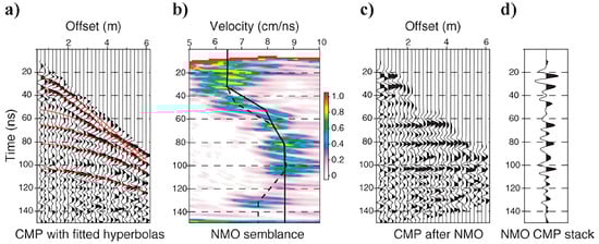
Figure 1.
(a) A CMP gather with six different reflections and their hyperbolic approximations (red lines); (b) the semblance spectrum, where the coherence of the data along hyperbolas associated with a variety of NMO velocities is depicted over time and best fitting velocities were picked for the six reflections and extrapolated and interpolated to a continuous velocity model (black line); (c) the CMP gather after NMO correction using this model; (d) the stacked trace. Figure taken from [6].
NMO correction with subsequent CMP stacking was often reviewed, updated, and extended (see, e.g., [7,8,9,10]). The Common Reflection Surface (CRS) stack method (see [11,12,13] and references given therein) constitutes one of the latest and probably the most successful generalizations of this technique. The CRS method extends CMP stacking towards the off-CMP dimension by adding a relative midpoint coordinate to the traveltime approximation. It provides a second-order approximation of the two-way traveltime of rays, reflected on a common reflection surface (3D seismic) or common reflection segment (2D seismic), respectively. The latter is depicted in Figure 2a as the red area around the normal incidence point R of the central ZO ray (straight blue line), which is defined by its emergence location x0 and traveltime t0. The same situation, but with inverted time axis, can be found in Figure 2b, where a collection of neighboring CMP gathers from near-surface seismic data is depicted side-by-side, in order to illustrate the continuation of reflection events in both midpoint and offset direction.
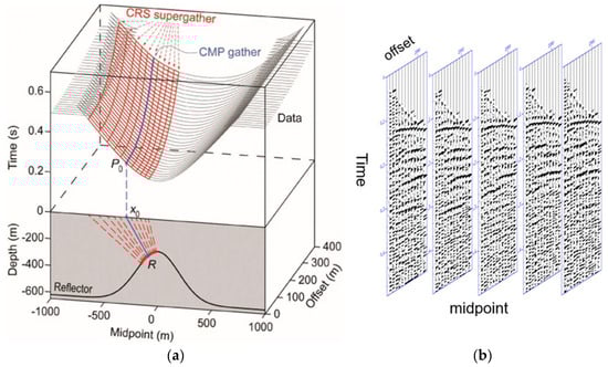
Figure 2.
(a) CRS stacking surface in the midpoint-offset domain, displayed above the corresponding 2D velocity medium composed of two constant velocity layers, separated by a dome shaped reflector. The gray curves are the forward modeled common-offset traveltimes for this interface. The stacking surface is depicted in red and spans over an entire collection of CMP gathers, a so-called CRS super-gather. All amplitudes summed along the red surface are assigned to the point P0 = (x0,t0), where x0 is the coincident source and receiver coordinate and t0 is the traveltime of the central ZO ray, depicted as a straight blue line (Figure modified from [14]). (b) A collection of neighboring CMP gathers from near-surface seismic data, showing the continuation of reflection events in both midpoint and offset direction.
For 2D acquisition on a plane surface without topography overlying an inhomogeneous but isotropic medium, according to [15], the hyperbolic CRS stacking operator in midpoint displacement, ∆xm, and half-offset, h, coordinates can be written as
with . The near-surface velocity in the vicinity of , , is assumed to be constant and a priori known. It plays the role of a constant of proportionality, allowing to parametrize a hyperbolic traveltime surface by three independent kinematic properties of the wavefield measured in : α, the emergence angle of the central ZO ray and and , the wavefront radii of two notional eigenwaves known as normal incident point (NIP) wave and normal (N) wave, as illustrated in Figure 3.
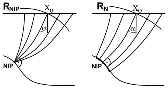
Figure 3.
Two eigenwaves described by the radii of curvature and . On the left, the NIP wave, related to a point source at the NIP, and, on the right, the N wave, related to an exploding reflector experiment around the NIP. Both wavefronts emerging at ZO location are depicted as arc segments with perpendicular rays (Figure modified from [16]).
These so-called CRS parameters represent the generalized counterpart to the NMO velocity which can be expressed as
Looking closer at how CRS stacking is actually implemented, we observe a basic difference to the conventional NMO/DMO correction plus CMP stack. Following the paradigm of data-driven imaging, an automated search for the optimum stacking parameter triple ) is performed for every sample of the output section instead of stacking with NMO velocities extrapolated and interpolated from a limited number of visually detectable reflection events, as portrayed in Figure 1. In other words, for every ZO sample , those values for , , and are searched for which parameterize the CRS traveltime surface, given by Equation (2), in such a way that it fits best to a measured reflection in the data. If does not lie on a reflection event, the attribute triple with the maximum coherence will nevertheless achieve only a relatively low coherence value and stacking will not result in a constructive summation of amplitudes.
A positive side-effect of treating every sample of the reflection event independently is that the so-called NMO-stretch (see Figure 1c, event four), which deteriorates the resulting stack section, is avoided [17]. This is because, unlike the conventional NMO velocity model shown in Figure 1b, the NMO velocity calculated from the CRS stacking parameters is generally neither constant for the entire duration of a reflection event nor does it increase due to velocity extra- or interpolation. Instead, it generally decreases with time from the top to the bottom of the event [16]. Why do we need NMO velocities that decrease over the wavelet to avoid the NMO stretch? Our hypothesis is that this results from the slightly unphysical way traveltimes are measured, according to which the last sample of the wavelet was not only recorded later but also has a larger traveltime than the first sample and thus has apparently traveled with a lower speed. Consequently, the NMO velocity must decrease towards the tail end of reflection events, as the apparent traveltime increases while the depth of the reflecting interface remains constant. This can also be seen from Equation (3), assuming a homogeneous layer with velocity over a horizontal interface. In this case, the ZO ray emerges vertically, i.e., α = 0. The NMO velocity is equal to if, and only if, is the exact time between the firing of the shot and the arrival of the head of the wavelet at the surface; only then holds. For the entire tail of the wavelet, which arrives later and corresponds to a larger , the NMO-velocity will be smaller than .
Fitting a surface in a three-dimensional data space can hardly be done by an interpreter and decisively not for every single image point of the ZO section. That is why such an entirely data-driven procedure has not been considered before the advent of data digitization and powerful computers. These technical breakthroughs were aided by scientific breakthroughs in the field of dynamic ray theory (see, [18] and references given therein) which finally allowed the substitution of the generic stacking parameters A, B, C, resulting from a second-order Taylor expansion in offset and midpoint, with physically interpretable quantities. The importance of this cannot be overstated since, for physically interpretable quantities, search ranges can be defined in a rational way and correlated properties, like the size of the projected Fresnel zone, the Common Reflection Point (CRP) trajectory, or the time-migrated image point location can be calculated (see, [19]). Having three instead of one physically meaningful stacking parameter also enabled the NIP wave tomography [20], the extension for rough surface topography [21], CRS-stack-based residual static corrections [22], pre-stack seismic data enhancement [23], and finally the CRP time migration without velocity model, presented in [24], which might be considered the capstone on top of the numerous applications that emerged from the CRS method. This paper is limited to the 2D case. For an overview of the 3D case, we like to refer the reader to [18,25,26] and references given therein.
2. Data-Driven Strategies for Stacking Parameter Estimation
At the beginning of this section, it is important to mention that anyone who wants to implement the 2D CRS stack method today can get by with a fraction of the processing steps that were originally necessary to compensate for limitations in processor number, speed and working memory. Only for very large 2D and particularly 3D datasets might it be too time consuming or expensive, even today, to search for all stacking parameters at the same time. Therefore, the strategy laid out in the following subsection still maintains some relevance even for readers who are not particularly interested in the implementational evolution of the method.
2.1. Pragmatic Search Strategy Plus Event-Consistent Smoothing
Around the year 2000, when the CRS stacking method was in its infancy, it was unfeasible to carry out for every sample of the ZO section a global simultaneous optimization of the full three-parameter reflection operator given by Equation (2). To overcome this impediment, ref. [12] developed and later also implemented a pragmatic search strategy. This cascaded strategy utilizes a sequential approach involving three global one-parameter line searches: the initial one conducted on individual CMP gathers, followed by two additional searches performed on a preliminary stack section generated as an outcome of the first search. Hoping that, by doing so, the proximity of the global coherence maximum is reached, the parameter search is concluded by a local three-parameter optimization utilizing the flexible polyhedron (Simplex) search by [27]. As a result, only local parameter optimization and stacking was carried out using the spatial operator.
It is evident that the success of this cascaded approach depends very much on the first step, called automatic CMP stack, where a preliminary ZO section is generated. However, the automatic CMP stack risks failing in cases of low signal-to-noise ratio and insufficient CMP fold; a risk especially high for small travel times where the range of usable offsets is very limited. Stacking along the NMO operator given by Equation (1), with only a few traces and unreliable NMO velocities, can create artificial gaps in the ZO image of reflection events or even result in a failure to image them at all.
The problems with outliers and fluctuations in the parameter values came fully into focus when a velocity model inversion method, called NIP wave tomography, was developed by [19], utilizing picked values of α and . To compensate for suboptimal parameters in limited areas of certain CMPs, ref. [28] introduced so-called event-consistent smoothing of stacking parameters, a post processing algorithm that takes advantage of the fact that, due to the predominantly layered structure of the subsurface, a smooth behavior of interfaces, and consequently also of stacking parameters, can be expected. Alexander Gerst, European Space Agency astronaut and commander of the International Space Station in 2018, implemented a first version of this approach as a student assistant, while studying geophysics at the University of Karlsruhe, Germany.
The smoothing algorithm is based on the combined application of mean and median filters within a rectangular box aligned with the underlying reflection event. The information on the slopes of events in the time domain is derived from the CRS parameters and allows avoidance of the mixing of intersecting events. As a result, the algorithm works in an event-consistent manner. It most often provides, even in case of conflicting dip situations, significantly improved parameter values. Any harm caused by the smoothing can be remediated by the subsequent application of local simultaneous three-parameter optimization. Typically, several iterations of smoothing and local optimization are carried out to obtain the best possible results.
The method was successfully employed in [29,30,31], and in various other examples. It proved to be especially beneficial in the case of complex near-surface conditions, which often lead to a strongly variable data quality [32]. In general, it can be concluded that, for hydrocarbon exploration (deep targets and large CMP fold), the shortcomings of the pragmatic search plus event-consistent smoothing are not very significant compared to the efficiency benefit obtained with respect to a global simultaneous search. However, for near-surface data, the same logic works but in the opposite direction: if the number of traces per CMP is low, the simultaneous search becomes easily affordable and highly beneficial for a stable and reliable estimation of the stacking parameter, particularly for complex structures and data with low signal-to-noise ratio.
2.2. Simultaneous Search Strategy
The pragmatic search strategy resulted from the need to employ computing resources in the most efficient way, necessitating a bulky and highly complex code. Later, with increasing processing power, it became more and more possible to shift the goal from an efficient to an effective implementation. The authors of [33] presented a global 1 × 3 parameter search applied to a small synthetic data set, using a simulated annealing strategy to find the optimum parameter triple. The same approach was later applied to real data by [34,35,36] carried out, for a synthetic dataset with a single dipping reflector, a systematic comparison between the pragmatic search strategy and a global 1 × 3 parameter search with a very fine grid. Ref. [37] applied a global 1 × 3 parameter grid-search with local optimization to very shallow SH-wave data from an urban environment with pronounced lateral velocity variations and low signal-to-noise ratio. Similarly, ref. [38] successfully employed a differential evolution global optimization algorithm without any velocity guide on challenging data sets with low-fold and low signal-to-noise ratio; in addition, ref. [39] used differential evolution for global CRS parameter optimization demonstrating that it provides significantly better parameters and improved stack results for complex salt bodies.
The concept of utilizing local slopes instead of coherence as an alternative strategy for stacking parameter estimation was first proposed by [40] and used in a global 3 × 1 parameter search scheme. Five years later, ref. [41] applied multi-dimensional local slopes for a global 1 × 3 parameter search in a real data study.
Estimating the effort of a global three-parameter simultaneous search in pre-stack data compared to a sequence of three line-searches in specific gathers involves consideration of two factors: firstly, the total number of coherency calculations required to create a stacked sample, and secondly, the number of traces included in each coherence calculation. For the simultaneous search, a 3D coherence matrix is computed where each value corresponds to a specific parameter combination, whereas, for the pragmatic search, three 1D coherence vectors are computed successively. In the simultaneous approach, all pre-stack traces within a spatial search aperture contribute to a single coherence calculation while, in the line searches, the search aperture is limited to either an offset range in a CMP gather or a midpoint range in the preliminary stacked section. Assuming a grid search with ten parameter values per dimension and neglecting iterative refinement steps, the simultaneous search requires 1000 coherence calculations, while the three subsequent line searches require only 30. Additionally, a single coherence calculation for a spatial operator in the pre-stack data covers approximately five CMP gathers on average, whereas each line search involves a number of traces comparable to one CMP gather. Based on these calculations, aiming at giving the reader a rough quantitative understanding of the relative numerical effort, the pragmatic search is estimated to be around 166 times faster than the simultaneous search.
Moore’s law can be used as a rough measure for how much computing power has increased since the first implementation of CRS stacking. It states that the number of transistors in a dense integrated circuit doubles about every two years (see: https://en.wikipedia.org/wiki/Moore%27s_law, accessed on 29 May 2024). Since transistors are also getting faster, computing power can roughly be assumed to double every 18 months. Consequently, computing power has grown at least by a factor of 1000, between the year 2000 and 2024. In addition, the available number of compute nodes, i.e., the number of basic units of computing infrastructure that provide processing power, memory, and sometimes storage for running individual tasks, is at least 10 if not 100 times higher today. Considering these factors, one can assume that processing a dataset using a full three-parameter global search is faster today than processing the same data set in the year 2000 using a 3 × 1 pragmatic search.
For the case study presented in Section 3, we utilize a global three-parameter grid-search with iterative refinement followed by a local flexible polyhedron search as reference. As a faster alternative, we apply a global diffraction plus local reflection search strategy, as discussed in the following section. For the computations, we use a Linux cluster, where we submit multiple instances of our code via the job scheduler. Each job is occupying itself only with a limited target zone of stacked CMPs. When the scheduler reports all jobs as finished, all results are first collected and then concatenated.
2.3. Hybrid Global Diffraction/Local Reflection Search
The N-wave is related to the so-called exploding reflector experiment. It emanates at the reflector with the curvature of a circular reflector element surrounding the NIP and propagates to the surface, where it reaches the ZO location with the radius of curvature . The NIP-wave instead, starts from a point source at the NIP and reaches with the radius of curvature . From these definitions, it follows that for a diffraction point is equal to . Therefore, substituting with transforms Equation (2) into the CRS diffraction operator ([19]), which reads
with .
Regarding global parameter search algorithms that employ a spatial operator, the computationally most efficient is the data-driven Common Diffraction Surface (CDS) stack developed by [42]. The CDS stack method utilizes the two-parameter diffraction operator given by Equation (4), but does not involve a search for α. Instead, the optimum (α) is determined for each α value on a predefined grid, before stacking in a DMO-like manner over all operators defined by the resulting α, (α) combinations, thereby reducing computational effort and resolving the conflicting dip problem. In [42], is renamed because, when fitting the diffraction operator to a reflection event, the resulting value for has not the exact physical meaning of , but represents a more generic stacking parameter.
Moving a step closer to the global 1 × 3 parameter optimization, ref. [43] introduced a global 2 + 1 parameter search method. It begins with a two-parameter search using the CRS diffraction operator, followed by a one-parameter search utilizing the full CRS reflection operator while maintaining the two previously determined parameters constant.
As a middle ground between the global simultaneous three-parameter search and the pragmatic search strategy, we propose a global simultaneous diffraction search as presented by [43], followed by a local three-parameter optimization that starts with as initial value for . In other words, the hybrid optimization algorithm that we propose in this paper consists of a global search assuming a diffraction, followed by a local search assuming a reflection. This makes sense considering that an arbitrarily located diffraction point and an arbitrarily located and oriented circular reflector segment are just two different levels of approximation of an unknown arbitrarily located, shaped and oriented subsurface reflector. Using as initial guess, is well justified by the NIP wave theorem [44], which states that the reflection traveltimes in the CMP gather are, up to the second order in half-offset h, equal to the diffraction traveltimes, which correspond to a diffractor at the normal incidence point (NIP) of the associated normal incidence ray. Furthermore, a sensibility analysis conducted by [45], depicted in Figure 4, shows that the CRS traveltime depends much more on the values of α and than on the value of the reflector curvature .
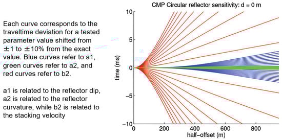
Figure 4.
Sensitivity analysis of the CRS traveltime with respect to reflector dip, reflector curvature and stacking velocity. Figure taken from [45].
Calculating the computational effort required for the global optimization, with the same assumptions that we made in the previous section, we have 100 coherence calculations for the simultaneous two-parameter search and end up with a computational effort that is about 16.6 times bigger than the effort of the pragmatic search strategy (see Table 1). In return, we obtain for the velocity analysis all benefits provided by a spatial operator that covers several CMP gathers.

Table 1.
Assuming a 10 point per dimension search grid without refinement and 5 CMP gathers per CRS/CDS aperture, we obtain the depicted values for the three methods discussed.
3. Shallow P-Wave Data Example
In the following we will conduct a detailed comparison between the three search strategies presented in the previous section. For this purpose, we reprocessed seismic line 2 of a P-wave data set acquired, processed and interpreted by [46]. CRS stack results for the less noisy line 1, obtained using the pragmatic search strategy, are discussed in [47]. The acquisition, which took place in the South-East of Sardinia, the second largest of Italy’s islands, can be categorized as a hydrogeological survey. In Sardinia, water is a precious resource, frequently in short supply during the long, hot, and dry summer, creating distribution conflicts between agriculture and tourism, as well as environmental problems, such as the salinization of coastal aquifers. The two lines, having a length of 1.1 km each, cross the coastal plain of the Flumendosa River, on the southeastern coast of Sardinia, Italy, roughly parallel to the coastline of the Tyrrhenian Sea. The survey was aiming both at imaging the Paleozoic bedrock topography, and at obtaining detailed structural and stratigraphic information on the sequence of largely fluvial sediments extending from the surface down to bedrock. The study aimed to gain a better understanding of the geological and hydrogeological factors influencing a highly productive aquifer located in thick Quaternary deposits and subject to extensive saltwater intrusion. For a detailed description of the geological and hydrogeological features of the target area we like to refer to [46].
The 89 shot-gathers were recorded using a standard common-midpoint (CMP) roll-along technique in an end-on configuration with 48 active 50-Hz geophones. At every shot point, 0.25-kg of explosives were fired. The sources were placed at a depth of 2 m, which lay in general below the water table. Geophone spacing of 5 m and source spacing of 10 m provided twelvefold CMP coverage with a CMP spacing of 2.5 m. The recorded traces had a sample interval of 0.5 ms and a record length of 1024 ms. Expecting a maximum reflector depth of 200–300 m a maximum source receiver offset of 245 m was chosen, which was right for line 2, where the maximum depth of the basement turned out to be ca. 200 m.
Three representative shot gathers, for the sake of simplicity called records in the following, are shown in Figure 5. In all records, the airwave (event e) is clearly visible. An up-dip reflector at the beginning of the line is presumably related to event f, with clear reversed moveout from record 3 and visible up to record 11. On the other end of the line where record 72 was selected as representative sample record, event g can be interpreted as refracted arrivals, stemming from a very shallow refractor, corresponding to the interface between the bedrock and the overlying sediments.
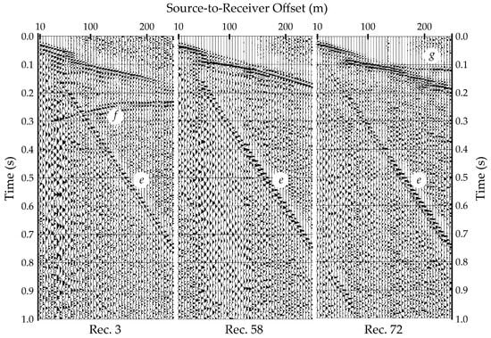
Figure 5.
Raw field records from three locations along the seismic line (see arrows in Figure 13a), according to [46]. Automatic Gain Correction (AGC) with a 100 ms time window was applied to enhance the different seismic events for the display.
Line 2 terminates on the southern bank of the Flumendosa River, 140 m from a Paleozoic outcrop. We chose line 2, because, of the two lines, it has the lower S/N ratio and is therefore better suited to highlight the benefits of a spatial velocity analysis. The annotated stack section produced by [46], and depicted in Figure 6, shows two dominant reflections. The first, event α, is the deepest coherent reflection in the section and was interpreted as the top of the Paleozoic bedrock, in accordance with the outcrop geology beyond the end of the line. It has an apparent dip to the north-northeast from about 290–165 ms two-way-traveltime (twtt) between CMP locations 10 and 60, before it gently shallows with a dip angle of about 10°, reaching 125 ms twtt at CMP 160. Even though less continuous and with lower amplitudes, event α can further be identified, from CMP 160 to the end of the line, with its change in reflection character probably caused by a change in reflectivity of the overlying sedimentary sequence. After CMP 160 event α abruptly starts descending until CMP 200, forming a trough with flat bottom between CDP 200–250, before it gently up-dips from 160 ms to 130 ms twtt at CMP 300. From CMP 300 to the end of the line, it continues to shallow, reaching 66 ms twtt, or a depth of approximately 52 m. The outcrop geology, and the velocity model depicted in Figure 13b, obtained by [46] from combining reflection-derived interval velocities and those derived from first-arrival information using refraction tomography, support the interpretation of event α as the top of the bedrock. The second of the two dominant reflection events is called event γ and is interpreted as the boundary between Holocene and Pleistocene alluvia. It starts at the beginning of the line and extends at least until CMP 340, where event α pinches out. It is nearly horizontal, with onset at 50–70 ms twtt. Event γ is overlain by seismic unit A that extends to the surface and consists of Holocene alluvial deposits composed of conglomerates, sands, and clays, according to samples obtained by drilling. Not all events in unit A can be interpreted as genuine reflections, because this very shallow part of the recordings is contaminated by various types of source-generated, high-amplitude coherent noise such as surface and refracted waves. Finally, at the left side of the section, unit B can be found between event γ and event α. Ref. [46] describes this unit as being composed of Pleistocene alluvial deposits.
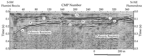
Figure 6.
Annotated stack section obtained by conventional NMO/DMO-Stack processing, published by [46].
For creating the series of CRS stacking results shown in Figure 7, Figure 8, Figure 9 and Figure 10, we used the following processing parameters. We chose a laterally constant near-surface velocity of 1600 m/s, consistent with the P-wave velocity of the water saturated sediments close to the ground surface. The total width of the coherence band was set to 33 samples, i.e., 0.0165 s. The offset aperture was 30 m for traveltimes up to 0.03 s and then increased linearly until the full offset range of 245 m was reached at 0.1 s. Roughly, this means that offsets do not become larger than two-times the reflector depth. The midpoint aperture increased linearly from the smallest to the largest traveltimes starting with 5 m halfwidth, i.e., 5 CDPs, and reaching finally 15 m halfwidth, i.e., 13 CDPs, for the maximum traveltime of 0.5 s. This means for the target area above the bedrock, i.e., 0 to 0.25 s, we have a midpoint aperture of 5 to 9 CDPs.
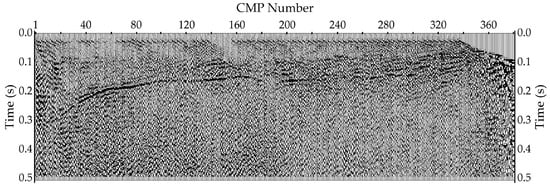
Figure 7.
Automatic CMP stack result obtained in step one of the cascaded search strategy.

Figure 8.
CRS stack result obtained after the cascaded search strategy.
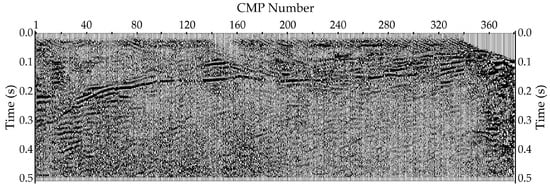
Figure 9.
CRS stack result after cascaded search strategy and local three-parameter optimization.
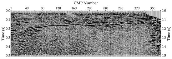
Figure 10.
CRS stack result after cascaded search plus three iterations of event-consistent smoothing, each followed by a local three-parameter optimization.
The CRS results presented in the following section are created in a fully data-driven way without the need of setting more than the above processing parameter values. We begin our comparison of the stack results with the automatic CMP stack result depicted in Figure 7. This section is the basis for the two subsequent search steps of the cascaded search strategy. The result of the complete three-step strategy is depicted in Figure 8. Figure 9 shows the stack result obtained from CRS stack using cascaded search followed by a local three-parameter optimization. Figure 10 shows the stack result obtained from CRS stack using cascaded search plus three iterations of event-consistent smoothing, each followed by a local three-parameter optimization. Now, coming to the simultaneous multi-parameter search strategies using spatial operators, we see in Figure 11 the result of the CRS stack using the hybrid diffraction/reflection search algorithm. Finally, all these results can be compared to the result of the CRS stack using simultaneous three-parameter search displayed in Figure 12.
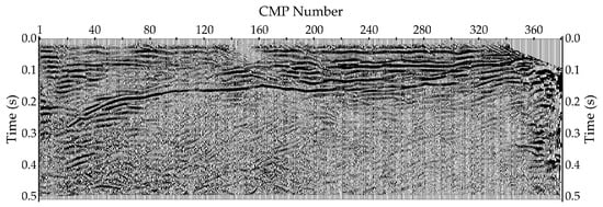
Figure 11.
CRS stack result after spatial hybrid diffraction/reflection parameter optimization.
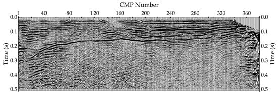
Figure 12.
CRS stack result after global simultaneous three-parameter optimization.
From Figure 7, Figure 8, Figure 9 and Figure 10, it is obvious how the stack quality slowly improves with every step of the cascaded imaging strategy, including event-consistent smoothing. The comparison between the stack section displayed in Figure 10 and those displayed in Figure 11 and Figure 12 shows clearly the superior reflection imaging capability of both global simultaneous search strategies. Not only reflections, but also diffractions, such as those at the left border (house wall) and in the center of the stack section (shallow object at the right end of the line), are more clearly imaged after velocity analysis with spatial operators.
Regarding the velocity analysis, the authors of [46] state: ”As is often the case, detailed velocity analysis proved to be the most important and time-consuming processing step. For both Lines 1 and 2, the initial velocity models were developed through integrated analysis of constant velocity gathers, constant velocity stacks, and semblance plots. Hand-picked direct arrivals supplied additional information on near-surface velocities.” This laborious and often quite subjective process must be kept in mind, when confronting the output shown in Figure 13 to the data-driven CRS results depicted in Figure 7, Figure 8, Figure 9, Figure 10, Figure 11, Figure 12, Figure 14, Figure 15, Figure 16 and Figure 17. In Figure 14, the NMO velocities obtained from the cascaded search followed by local optimization are displayed, while in Figure 15 we display the NMO velocities obtained from the cascaded search plus three iterations of event-consistent smoothing, each followed by a local optimization. In Figure 16, the NMO velocities from the hybrid diffraction/reflection search are shown and in Figure 17 the NMO velocities from the full simultaneous three-parameter search. In all the CRS stack examples, the NMO velocities were calculated according to Equation (3) from the estimated CRS parameters.
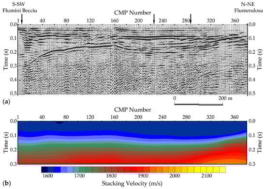
Figure 13.
CMP stack after NMO/DMO processing (a) and the respective stacking velocities after DMO (b). Figure modified from [46].
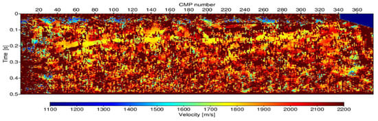
Figure 14.
CRS NMO velocities obtained from cascaded search followed by local optimization.
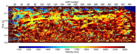
Figure 15.
CRS NMO velocities obtained from cascaded search plus three iterations of event-consistent smoothing, each followed by a local three-parameter optimization.
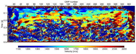
Figure 16.
CRS NMO velocities obtained from hybrid diffraction/reflection parameter optimization.
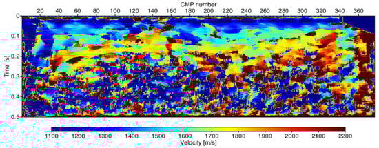
Figure 17.
CRS NMO velocities obtained from full simultaneous three-parameter search.
Comparing the NMO velocities in Figure 14 and Figure 15 and those in Figure 16 and Figure 17 demonstrates the superior accuracy of the global simultaneous search strategies in estimating NMO velocities and the underlying stacking parameters α and RNIP. In addition, diffractions, such as those at the left border (house wall) and in the center of the stack section (shallow object at the right end of the line), are much more clearly imaged.
4. Discussion
If we compare Figure 7 and Figure 13b, it is obvious that the automatic CMP stack used as the first step of the pragmatic search strategy is far less successful than the conventional CMP stack methodology. For the making of this judgment, we assume a minor influence of the DMO procedure that was applied in Figure 13b, but not in Figure 14. In general, one can conclude from Figure 7 that the automatic CMP stack was only successful in imaging event α, and mainly on the left half of the section. Interestingly, the relatively strong reflection imaged above event α, around CMP 140, may be connected to event γ, which is not present in the original CMP stack results. The general picture gets a little bit clearer in Figure 8, where the CRS operator was used for stacking based on the parameter values estimated by the cascaded search strategy. The improvement of the S/N ratio is notable, which helps to uncover some parts of event α on the right side of the section. Particularly there, on the right side above event α, traces of event γ emerge from the noise. The enhancement obtained from a subsequent local three-parameter optimization is clearly visible in Figure 9. Reflections become slightly more pronounced, and the traces of shallow events show up above event α. Going on to Figure 10, the improved lateral event-continuity resulting from the three iterations of event-consistent smoothing of the stacking parameters followed by local three-parameter optimization is notable. In Figure 11, where the CRS stack result using the hybrid diffraction/reflection search algorithm is displayed, the picture changes relatively drastically. Event γ becomes quite clearly observable over the whole section, except for the area between CMP 100 and 130. In addition, event α can be traced now through the whole section. Even the gap around CMP 240 is covered, but is still not as well defined as the rest of event α. Finally, the stack section displayed in Figure 12, resulting from the full simultaneous three-parameter search, is the best image we obtained for this data, but outperforms the stack result displayed in Figure 11, only in tiny details. In both Figure 11 and Figure 12, an ultra-shallow horizontal event, which might belong to seismic unit A, can be seen throughout the whole section except in the area between CMPs from 140 to 160. This gap in the continuity of the event is probably due to the bad quality of seismic signals, which not even the simultaneous three-parameter CRS stack was able to improve. However, as mentioned in the original publication of [46], these very early traveltimes are not very reliable since the usable stacking aperture in offset direction is extremly narrow. Furthermore, comparing Figure 12 (or even Figure 11) and Figure 13a, it is obvious that, relative to the NMO/DMO stack, the CRS stack is better able to image the internal layering of unit B, at least beyond CMP 160. In the first part of the section the internal structures of unit B are not as evident, probably due to a lack of data resolution and/or low data quality.
Coming to the NMO velocities, we will start with Figure 14, which displays NMO velocities calculated from CRS parameters estimated using the cascaded search strategy. Here, we have first to state that, in this section, the deep blue color on the upper right edge is used as no-value flag, while the deep brownish color in the rest of the section can be seen as the no-useful-value flag, since the coherence analysis tends to favor very high NMO velocities, i.e., a flat traveltime assumption, in the absence of detectable events. Having said this, we can state that, in Figure 14, well defined velocities are mainly available for event α and predominantly on the left side of the section. The picture could even lead to the wrong impression that there would be a steeper reflector below the event α pinching out at CDP 280. This continues to be true for Figure 15, where the NMO velocities after cascaded search plus three iterations of event-consistent smoothing, each followed by a local three-parameter optimization, are displayed. A certain success of the strategy is clearly observable, as could be expected from the improved stack result. Nevertheless, there are still too many samples for which no proper value could be determined despite the elaborate optimization strategy. Figure 16 and Figure 17 shows a totally different picture. Searching directly with a spatial operator that spans over several CMP gathers creates a continuity of the NMO velocity values, which is consistent with the integral nature of this parameter that makes drastic variations from one sample to the other impossible. The dark brownish samples at the borders of the section still correspond to no useful values.
5. Conclusions
In the last decades, computing power has increased drastically. As we have laid out in detail, imaging methods have now become affordable, which directly optimize spatial stacking operators for maximum coherence within the pre-stack data. The benefit–cost ratio is particularly attractive for near-surface seismics. A global simultaneous grid search enables the comprehensive evaluation of a wide range of velocity model configurations. By systematically testing various combinations of three stacking parameters, the presented CRS stack approach identifies the parametrization that optimally describes a seismic reflection event in midpoint and offset dimensions. The iterative refinement process incorporates both global and local searches to ensure a computationally efficient approach while maintaining high accuracy. The global search identifies promising regions in the stacking parameter space, while the subsequent local optimization fine-tunes the parameters for the stacking process. To achieve a well-balanced compromise between computational efficiency and stacking parameter quality, we presented a hybrid method, which combines a global search for the two parameters of the CDS operator with a local optimization of the three parameters of the CRS operator. Using the global simultaneous three-parameter optimization as reference, we showed that this global-diffraction/local-reflection search algorithm can deliver nearly identical results, while reducing the computational cost by an order of magnitude. As a case study, we presented data from a hydrogeological survey, targeting the definition of predictive groundwater flow models for effective water resource management. A comprehensive comparison with results of conventional methods demonstrated the significant improvement in resolution and reflection continuity that can be obtained, together with a far more accurate velocity field, by using CRS stacking with spatial velocity analysis. The method clearly imaged two key reflection events γ and α, interpreted as the boundary between Holocene and Pleistocene alluvia and the top of the Paleozoic bedrock, respectively, in a fully data driven way, despite the challenges posed by the noisy low-fold near-surface data.
Author Contributions
Conceptualization, Z.H. and G.P.D.; methodology, Z.H.; software, Z.H.; validation, G.P.D. and Z.H; formal analysis, Z.H; investigation, Z.H.; resources, G.P.D. and Z.H.; data curation, G.P.D.; writing—original draft preparation, Z.H.; writing—review and editing; Z.H and G.P.D.; visualization, Z.H. and G.P.D.; supervision, Z.H. and G.P.D.; project administration, Z.H. and G.P.D.; funding acquisition, Z.H. and G.P.D. All authors have read and agreed to the published version of the manuscript.
Funding
This research was funded by the Autonomous Region of Sardinia grant number ex art. 9 L.R. 20/2015, and the APC was funded by the University of Cagliari.
Data Availability Statement
The data presented in this study are available on request from the corresponding author.
Acknowledgments
The authors are grateful to Guido Satta for valuable discussions and to an anonymous reviewer whose detailed and constructive feedback strengthened this work.
Conflicts of Interest
The authors declare no conflicts of interest.
References
- Kravtsov, Y.A.; Orlov, Y.L. Geometrical Optics of Inhomogeneous Media; Springer Verlag: New York, NY, USA, 1990; ISBN 9783642840333. [Google Scholar]
- Mayne, W.H. Common reflection point horizontal data stacking techniques. Geophysics 1962, 27, 927–938. [Google Scholar] [CrossRef]
- Dix, C.H. Seismic velocities from surface measurements. Geophysics 1955, 20, 68–86. [Google Scholar] [CrossRef]
- Neidell, N.S.; Taner, M.T. Semblance and other coherency measures for multichannel data. Geophysics 1971, 36, 482–497. [Google Scholar] [CrossRef]
- Deregowski, S.M. What is DMO? First Break 1986, 4, 7–24. [Google Scholar] [CrossRef]
- Perroud, H.; Tygel, M. Velocity estimation by the common-reflection-surface (CRS) method: Using ground-penetrating radar data. Geophysics 2005, 70, B43–B52. [Google Scholar] [CrossRef]
- Castle, R.J. A theory of normal moveout. Geophysics 1994, 59, 983–999. [Google Scholar] [CrossRef]
- Schwarz, B. Moveout and Geometry. Ph.D. Thesis, University of Hamburg, Hamburg, Germany, 2015. [Google Scholar]
- Walda, J.; Schwarz, B.; Gajewski, D. A competitive comparison of multi-parameter stacking approaches. In Proceedings of the 78th EAGE Conference and Exhibition 2016: Efficient Use of Technology–Unlocking Potential; EAGE (European Association of Geoscientists and Engineers): Vienna, Austria, 2016; Volume 2016, pp. 1–5. [Google Scholar] [CrossRef]
- Schwarz, B.; Gajewski, D. A generalized view on normal moveout. Geophysics 2017, 82, V335–V349. [Google Scholar] [CrossRef]
- Höcht, G.; De Bazelaire, E.; Majer, P.; Hubral, P. Seismics and optics: Hyperbolae and curvatures. J. Appl. Geophys. 1999, 42, 261–281. [Google Scholar] [CrossRef]
- Mann, J.; Jäger, R.; Müller, T.; Höcht, G.; Hubral, P. Common-reflection-surface stack—A real data example. J. Appl. Geophys. 1999, 42, 301–318. [Google Scholar] [CrossRef]
- Hertweck, T.; Schleicher, J.; Mann, J. Data stacking beyond CMP. Lead. Edge 2007, 26, 818–827. [Google Scholar] [CrossRef]
- Müller, T. The Common Reflection Surface Stack Method: Seismic Imaging without Explicit Knowledge of the Velocity Model. Ph.D. Thesis, University of Karlsruhe, Karlsruhe, Germany, 1999. [Google Scholar]
- Jäger, R.; Mann, J.; Höcht, G.; Hubral, P. Common-reflection-surface stack: Image and attributes. Geophysics 2001, 66, 97–109. [Google Scholar] [CrossRef]
- Duveneck, E. Velocity model estimation with data-derived wavefront attributes. Geophysics 2004, 69, 265–274. [Google Scholar] [CrossRef]
- Mann, J.; Höcht, G. Pulse Stretch Effects in the Context of Data-Driven Imaging Methods. In Proceedings of the 65th EAGE Conference & Exhibition; European Association of Geoscientists & Engineers: Stavanger, Norway, 2003; p. cp-6-00405. [Google Scholar] [CrossRef]
- Höcht, G. Traveltime Approximations for 2D and 3D Media and Kinematic Wavefield Attributes. Ph.D. Thesis, University of Karlsruhe, Karlsruhe, Germany, 2002. [Google Scholar]
- Mann, J. Extensions and Applications of the Common-Reflection-Surface Stack Method. Ph.D. Thesis, University of Karlsruhe, Karlsruhe, Germany, 2002. [Google Scholar]
- Duveneck, E.; Hubral, P. Tomographic velocity model inversion using kinematic wave field attributes. In Proceedings of the 72nd SEG Annual Meeting; Society of Exploration Geophysicists: Salt Lake City, UH, USA, 2002; Volume 21, pp. 862–865. [Google Scholar] [CrossRef]
- Zhang, Y. Common-Reflection-Surface Stack and the Handling of top Surface Topography; Logos-Verl: Berlin, Germany, 2003; ISBN 978-3-8325-0298-0. [Google Scholar]
- Koglin, I.; Mann, J.; Heilmann, Z. CRS-stack-based residual static correction. Geophys. Prospect. 2006, 54, 697–707. [Google Scholar] [CrossRef]
- Baykulov, M.; Gajewski, D. Prestack seismic data enhancement with partial common-reflection-surface (CRS) stack. Geophysics 2009, 74, V49–V58. [Google Scholar] [CrossRef]
- Coimbra, T.A.; Faccipieri, J.H.; Rueda, D.S.; Tygel, M. Common-reflection-point time migration. Stud. Geophys. Geod. 2016, 60, 500–530. [Google Scholar] [CrossRef]
- Bergler, S.; Hubral, P.; Marchetti, P.; Cristini, A.; Cardone, G. 3D common-reflection-surface stack and kinematic wavefield attributes. Lead. Edge 2002, 21, 1010–1015. [Google Scholar] [CrossRef]
- Xie, Y. Determination and Application of 3-D Wavefront Attributes. Ph.D. Thesis, University of Hamburg, Hamburg, Germany, 2017. [Google Scholar]
- Nelder, J.A.; Mead, R. A Simplex Method for Function Minimization. Comput. J. 1965, 7, 308–313. [Google Scholar] [CrossRef]
- Mann, J.; Duveneck, E. Event-consistent smoothing in generalized high-density velocity analysis. In Proceedings of the 73rd Annual SEG Meeting; Society of Exploration Geophysicists: Dallas, TX, USA, 2004; Volume 23, pp. 2176–2179. [Google Scholar] [CrossRef]
- Heilmann, Z.; Mann, J.; Duveneck, E.; Hertweck, T. CRS-Stack-Based Seismic Reflection Imaging–A Real Data Example. In Proceedings of the 66th EAGE Conference & Exhibition; European Association of Geoscientists & Engineers: Paris, France, 2004; p. cp-3-00429. [Google Scholar] [CrossRef]
- Klüver, T.; Mann, J. Event-consistent smoothing and automated picking in CRS-based seismic imaging. In Proceedings of the 75th SEG International Exposition and Annual Meeting; Society of Exploration Geophysicists: Houston, TX, USA, 2005; pp. 1894–1897. [Google Scholar] [CrossRef]
- Deidda, G.P.; Battaglia, E.; Heilmann, Z. Common-reflection-surface imaging of shallow and ultrashallow reflectors. Geophysics 2012, 77, B177–B185. [Google Scholar] [CrossRef][Green Version]
- Heilmann, Z.; Mann, J.; Koglin, I. CRS-stack-based seismic imaging considering top-surface topography. Geophys. Prospect. 2006, 54, 681–695. [Google Scholar] [CrossRef]
- Garabito, G.; Ao, J.; Cruz, C.R.; Hubral, P. 2-D CRS Stack: One-step versus multi-step strategies. In Proceedings of the 10th International Congress of the Brazilian Geophysical Society & EXPOGEF; Society of Exploration Geophysicists: Rio de Janeiro, Brazil, 2007; pp. 1497–1500. [Google Scholar] [CrossRef]
- Garabito, G.; Stoffa, P.L.; Ferreira, C.A.S.; Cruz, J.C.R. Part II—CRS-beam PSDM: Kirchhoff-beam prestack depth migration using the 2D CRS stacking operator. J. Appl. Geophys. 2012, 85, 102–110. [Google Scholar] [CrossRef]
- Minato, S.; Tsuji, T.; Matsuoka, T.; Nishizaka, N.; Ikeda, M. Global optimisation by simulated annealing for common reflection surface stacking and its application to low-fold marine data in southwest Japan. Explor. Geophys. 2012, 43, 59–69. [Google Scholar] [CrossRef]
- Barros, T.; Ferrari, R.; Krummenauer, R.; Lopes, R.; Tygel, M. The Impact of the Parameter Estimation Strategy in the CRS Method. In Proceedings of the 13th International Congress of the Brazilian Geophysical Society & EXPOGEF; Society of Exploration Geophysicists: Rio de Janeiro, Brazil, 2013; pp. 1534–1539. [Google Scholar] [CrossRef]
- Heilmann, Z.; Müller, H.-P.; Satta, G.; Deidda, G.P. Real-time or Full-precision CRS Imaging Using a Cloud Computing Portal—Multi-offset GPR and Shear-wave Reflection Data. In Proceedings of Near Surface Geoscience 2014—20th European Meeting of Environmental and Engineering Geophysics; European Association of Geoscientists & Engineers: Athens, Greece, 2014; pp. 1–5. [Google Scholar] [CrossRef]
- Barros, T.; Ferrari, R.; Krummenauer, R.; Lopes, R. Differential evolution-based optimization procedure for automatic estimation of the common-reflection surface traveltime parameters. Geophysics 2015, 80, WD189–WD200. [Google Scholar] [CrossRef]
- Walda, J.; Gajewski, D. Common-reflection-surface stack improvement by differential evolution and conflicting dip processing. In Proceedings of the SEG Technical Program Expanded Abstracts; Society of Exploration Geophysicists: Salt Lake City, UH, USA, 2015; Volume 34, pp. 3842–3847. [Google Scholar] [CrossRef]
- Santos, L.T.; Schleicher, J.; Costa, J.C.; Novais, A. Fast estimation of CRS parameters using local slopes. In Proceedings of the SEG Technical Program Expanded Abstracts; Society of Exploration Geophysicists: Houston, TX, USA, 2009; pp. 3735–3739. [Google Scholar] [CrossRef]
- Hellman, K. Simultaneous estimation of CRS parameters with multi-dimensional local slopes. In Proceedings of the 84th Annual SEG Meeting; Society of Exploration Geophysicists: Salt Lake City, UH, USA, 2014; pp. 4686–4690. [Google Scholar] [CrossRef]
- Soleimani, M.; Piruz, I.; Mann, J.; Hubral, P. Common reflection surface stack; accounting for conflicting dip situations by considering all possible dips. J. Explor. Geophys. 2009, 18, 271–288. [Google Scholar]
- Garabito, G.; Cruz, J.C.; Hubral, P.; Costa, J. Common reflection surface stack: A new parameter search strategy by global optimization. In Proceedings of the 70th SEG Annual Meeting; Society of Exploration Geophysicists: Calgary, AB, Canada, 2001; Volume 20, pp. 2009–2012. [Google Scholar] [CrossRef]
- Hubral, P. Computing true amplitude reflections in a laterally inhomogeneous earth. Geophysics 1983, 48, 1051–1062. [Google Scholar] [CrossRef]
- Perroud, H.; Krummenauer, R.; Tygel, M.; Lopes, R.R. Parameter estimation from non-hyperbolic reflection traveltimes for large aperture common midpoint gathers. Near Surf. Geophys. 2014, 12, 679–687. [Google Scholar] [CrossRef]
- Deidda, G.P.; Ranieri, G.; Uras, G.; Cosentino, P.; Martorana, R. Geophysical investigations in the Flumendosa River Delta, Sardinia (Italy)–Seismic reflection imaging. Geophysics 2006, 71, B121–B128. [Google Scholar] [CrossRef]
- Heilmann, Z.; Deidda, G.P.; Satta, G.; Bonomi, E. Real-time imaging and data analysis for shallow seismic data using a cloud-computing portal. Near Surf. Geophys. 2013, 11, 407–422. [Google Scholar] [CrossRef]


Disclaimer/Publisher’s Note: The statements, opinions and data contained in all publications are solely those of the individual author(s) and contributor(s) and not of MDPI and/or the editor(s). MDPI and/or the editor(s) disclaim responsibility for any injury to people or property resulting from any ideas, methods, instructions or products referred to in the content. |
© 2024 by the authors. Licensee MDPI, Basel, Switzerland. This article is an open access article distributed under the terms and conditions of the Creative Commons Attribution (CC BY) license (https://creativecommons.org/licenses/by/4.0/).