Reconstruction of High-Frequency Bridge Responses Based on Physical Characteristics of VBI System with BP-ANN

Featured Application

This work might be applied to long-term bridge health monitoring, including missing data reconstruction and bridge service status investigation, with short-term monitoring data.

Abstract

Response reconstruction is essential in bridge health monitoring for recovering missing data and evaluating service status. Previous studies have focused on reconstructing responses at specific cross-sections using data from adjacent sections. To address this challenge, time-series prediction methods have been employed for response reconstruction. However, these methods often struggle with the inherent complexities of long-term time-varying traffic conditions, posing practical challenges. In this study, we analyzed the theoretical physical characteristics of high-frequency bridge dynamics within a simplified vehicle–bridge interaction (VBI) system. Our analysis revealed that the relationship between high-frequency bridge responses across different cross-sections is time-invariant and only dependent on the bridge’s mode shape. This relationship remains unaffected by time-varying factors such as traffic loading and environmental conditions like air temperature. Based on these physical characteristics, we propose the backpropagation artificial neural network (BP-ANN) method for response reconstruction. The validity of these physical characteristics was confirmed through finite element models, and the effectiveness of the proposed method was demonstrated using field test data from a continuous bridge. Our verification results show that the BP-ANN method enables effective utilization of short-term monitoring data for long-term bridge health monitoring, without necessitating real-time adjustments for factors such as traffic conditions or air temperature.

1. Introduction

Bridge response reconstruction is crucial for bridge health monitoring [1], aiming to predict responses at specific locations using data from other locations. By leveraging historical monitoring data from multiple locations of the bridge, a relationship [2] can be established to map responses across these locations. This relationship allows current monitoring data from multiple locations to reconstruct the response at a specific location. If the deviation between the reconstructed response and actual monitoring data exceeds a predefined threshold, it may signal potential bridge damage [3]. Response reconstruction has been integrated into numerous bridge health monitoring systems [4] for the data recovery and evaluation of bridge service status.

Scholars have proposed several methodologies to model this relationship, categorized into two main types: model-based and data-driven approaches. Model-based methods [5,6,7] involve constructing finite element models and applying external loads to predict responses at specified cross-sections. However, due to discrepancies between design and actual conditions, creating an accurate finite element model via general model updating methods can be time-consuming. Moreover, estimating or measuring external loads may yield imprecise results, limiting the applicability of model-based approaches in practical engineering scenarios.

In contrast, data-driven techniques simulate relationships [8,9] directly using signals measured from different cross-sections. These methods typically involve deriving bridge mode shapes and using them with corresponding measured amplitudes to reconstruct responses across the entire structure. Widely used methods such as stochastic subspace identification (SSI) [10,11] and the eigensystem realization algorithm [12,13] have been developed and applied. However, mode shape identification poses an inverse problem, and existing methods [10,11,12,13] rely on inverse calculations that can be sensitive to measurement noise. Consequently, these approaches may not be sufficiently effective for medium- and short-span bridges with low signal-to-noise ratios (SNRs), making accurate results challenging to obtain. Furthermore, ensuring the accuracy of identification processes often requires deploying a significant number of sensors.

Recent years have seen significant progress in data-driven approaches, especially in machine learning techniques, which have proven advantageous in solving inverse problems [14]. In the context of bridge response reconstruction, traditional methods have been replaced by machine learning algorithms like LSTM networks [15], CNNs [16], and GANs [17]. These methods simulate direct relationships between signals using training data to generate time-series bridge responses. For instance, Zhang et al. [18] developed a ConvLSTM network to extract spatiotemporal features and forecast structural responses. Tian [19] used Bilateral LSTM networks to correlate beam deflection and cable tension in cable-stayed bridges based on sensor data. Ni [20] employed CNNs to approximate mappings among bridge responses, facilitating deflection reconstruction from alternative measurements. Oh [21] proposed and validated an optimal CNN architecture for reconstructing beam-like structure responses through experiments. Additionally, Oh [22] used CNNs to link structural responses with ambient air temperature. Jiang [23] introduced a GAN-based method for reconstructing vehicle-induced strain, considering spatial–temporal relationships with other strain sensors. Fan [24] applied a Self-Attention GAN (SAGAN) to learn correlations and reconstruct structural responses from precise monitoring data. Moreover, GANs have been used in bridge Weight-in-Motion (WIM) systems [25] to reconstruct bridge responses, highlighting traffic flow variations across different months.

Nevertheless, time-series forecasting techniques require substantial data to construct predictive models that map inputs to outputs. These models must account for temporal variables, including seasonal and daily changes in air temperature and traffic volume, as noted in [26,27,28]. For long-term monitoring, significant shifts in these conditions are expected. Thus, these methods demand comprehensive data over an extended period, which can be difficult to obtain if the monitoring data are limited or incomplete.

This study aims to reconstruct the high-frequency responses induced by vehicles in short- and medium-span bridges and explores the feasibility of using short-term monitoring data for long-term data reconstruction. A theoretical analysis was conducted to understand the physical behavior of high-frequency bridge responses within a simplified vehicle–bridge interaction (VBI) system [29]. A VBI system, as outlined in [30], includes a beam, a vehicle, and tire–bridge road surface interaction. We derived theoretical dynamic responses from dynamic equations of the VBI system, particularly focusing on the transfer function of high-frequency responses across different bridge sections. The findings indicated that the relationship remained stable over time, unaffected by traffic and temperature changes, and was determined solely by the bridge mode shape. Numerical simulations were proposed to test this hypothesis. Based on these characteristics, response reconstruction is treated as a regression problem. The backpropagation artificial neural network (BP-ANN), known for its effectiveness in regression tasks as cited in [31,32,33,34], was utilized for reconstructing high-frequency responses. Unlike other time-series prediction methods, the BP-ANN does not consider a temporal component, which is consistent with the time-invariant nature of the target relationship. The trained neural network enables the reconstruction of responses at a specific section based on data from other sections. Field experiment monitoring data were used to validate the BP-ANN’s performance and to confirm the potential of using short-term monitoring data to develop a model for long-term monitoring reconstruction.

Section 2 examines the physical characteristics of a simple VBI system, specifically the time-invariant relationship between high-frequency responses at different cross-sections. Additionally, it outlines the application strategy of the BP-ANN. Section 3 further examines the target relationship through a series of finite element simulations. Section 4 tests the proposed method with the field monitoring data.

2. Methodology

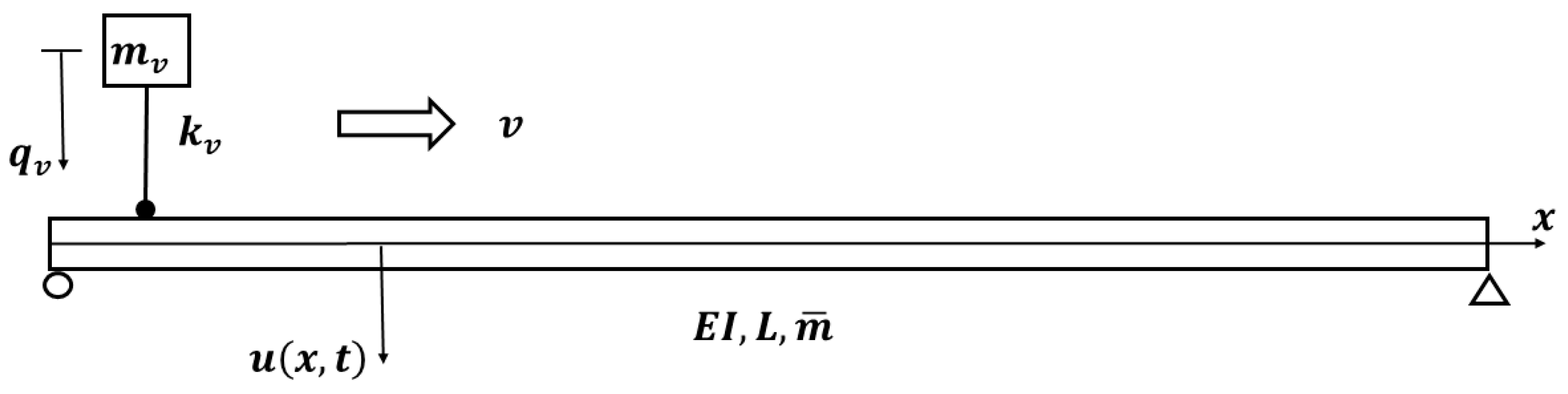
2.1. Dynamics of a VBI System

The theoretical dynamics of a simple VBI system were investigated. As depicted in Figure 1, the vehicle was simplified as a moving sprung mass, and the bridge is a simple supported beam. The vehicle moves with a constant speed v. The dynamic equation [35] of the vehicle is illustrated as Equation (1):

$$m_v{\ddot{q}}_v+k_v{q}_v=k_v{\left.u\right|}_{x=vt}$$

(1)

where $m_v$ denotes the mass of the vehicle, $k_v$ represents the stiffness of the spring, $q_v$ is the vertical displacement of the vehicle, and ${\ddot{q}}_v$ is the corresponding vehicle acceleration. $u(x,t)$ denotes the vertical displacement of the bridge at $x$ on the time point $t$. The initial configuration is that the vehicle is situated at the far end of the beam. The initial beam deflection under gravity was not considered for the purposes of simplification [35]. The displacement of the bridge and the vehicle is in a downward direction.

The dynamic equations of the beam are the following [35]:

$$\overline{m}\ddot{u}+EI{u}^{″″}=p\left(x,t\right)$$

(2a)

$$p\left(x,t\right)=[-m_{v}g+k_v{\left.(q_v-u\right|}_{x=vt})\left]\delta \right(x-vt)$$

(2b)

where $\overline{m}$ denotes the mass of the bridge per unit length, $E$ is the elastic modulus, and $I$ represents the moment of inertia of the beam cross-section. $L$ is the span of the beam, and $p(x,t)$ is the interaction force applied on the bridge through the contact between the tire and bridge. In this simplified model [35], the contact region between the tire and the bridge surface was simplified as a contact point. $\ddot{u}$ denotes the second derivative of displacement with respect to time, and $u^{″″}$ denotes the fourth derivative of displacement with respect to $x$. $g$ is the gravitational acceleration, and $\delta (x-vt)$ is the Dirac delta function evaluated at the contact point, x = vt.

By assuming that the vehicle mass was much smaller than the bridge mass, Yang and Lin [35] derived the theoretical dynamic responses of the bridge (illustrated as Equation (3)):

$$u\left(x,t\right)=\sum _n{\displaystyle \frac{{\Delta }_{stn}}{1-S_n^2}}\{sin{\displaystyle \frac{n\pi x}{L}}[\mathrm{s}\mathrm{i}\mathrm{n}{\displaystyle \frac{n\pi vt}{L}}-S_n\sin {\omega }_{bn}t]\}$$

(3)

where $n$ ($n=\mathrm{1,2},3,\dots$) denotes the mode order and ${\omega }_{bn}$ is the n-th bridge natural vibrational frequency. In detail,

$${\Delta }_{st,n}={\displaystyle \frac{-2m_{v}g{L}^3}{n^4{\pi }^{4}EI}}$$

(4a)

$$S_n={\displaystyle \frac{n\pi v}{L{\mathsf{\omega }}_{b,n}}}$$

(4b)

$${\mathsf{\omega }}_{b,n}={\displaystyle \frac{n^2{\pi }^2}{L^2}}\sqrt{{\displaystyle \frac{EI}{\overline{m}}}}$$

(4c)

in which $g$ is the gravitational acceleration.

The effects of damping on the vehicle and the beam were omitted from the analysis. Equation (3) [35], derived from the simplified model that treats a vehicle as a moving force $-m_{v}g$, inherently neglects the damping effect of the vehicle. Moreover, as the vehicle traverses the beam, the interaction force persistently stimulates the beam’s oscillations. The damping effect of the bridge, in the context of bridge dynamics, is not conspicuously evident. As a result, the damping influence of the bridge was similarly disregarded in this study.

The $u\left(x,t\right)$ in Equation (3) was divided as a low-frequency component $u_{low}\left(x,t\right)$ and a high-frequency component $u_{high}\left(x,t\right)$ (shown in Equation (5a) and (5b)).

$$u_{low}\left(x,t\right)=\sum _n{\displaystyle \frac{{\Delta }_{stn}}{1-S_n^2}}\left[sin{\displaystyle \frac{n\pi x}{L}}\sin {\displaystyle \frac{n\pi vt}{L}}\right]$$

(5a)

$$u_{high}\left(x,t\right)=\sum _n{\displaystyle \frac{{\Delta }_{stn}}{1-S_n^2}}[-sin{\displaystyle \frac{n\pi x}{L}}{S}_n\sin {\omega }_{b,n}t]$$

(5b)

This division is predicated on the variance in the frequency spectrum that distinguishes these two components. For $u_{low}\left(x,t\right)$, the vibrational frequency is ${\displaystyle \frac{n\pi v}{L}}$ and is determined by the moving speed of the vehicle. Therefore, this frequency is named the “Driving-force frequency” [35]. Meanwhile, $u_{high}\left(x,t\right)$ represents vibrations that correspond to the natural vibrational modes of the bridge $\sin {\omega }_{bn}t$. According to Yang and Lin [35] and Paultre [36], the frequencies of the first several driving-force modes are considerably lower than those of the first natural vibrational modes. In this study, the “high-frequency responses” refer to the vibrations that matched the bridge’s natural vibrational frequencies. Additionally, a high-pass filter was utilized to extract the high-frequency vibrational component from the direct monitoring data.

From Equation (5a), the high-frequency displacements at three distinct cross-sections, specifically at $x_1$, $x_2$, and $x_3$, were derived as the following:

$$\begin{gathered} -\left[\begin{array}{cccc}sin{\displaystyle \frac{\pi x_1}{L}}& sin{\displaystyle \frac{2\pi x_1}{L}}& \cdots & sin{\displaystyle \frac{n\pi x_1}{L}}\\ sin{\displaystyle \frac{\pi x_2}{L}}& sin{\displaystyle \frac{2\pi x_2}{L}}& \cdots & sin{\displaystyle \frac{n\pi x_2}{L}}\\ sin{\displaystyle \frac{\pi x_3}{L}}& sin{\displaystyle \frac{2\pi x_3}{L}}& \cdots & sin{\displaystyle \frac{n\pi x_3}{L}}\end{array}\right]\left[\begin{array}{cccc}{\displaystyle \frac{{∆}_{st,1}}{1-S_1^2}}{S}_{1}sin{\omega }_{b,1}{t}_0& {\displaystyle \frac{{∆}_{st,1}}{1-S_1^2}}{S}_{1}sin{\omega }_{b,1}{t}_1& \cdots & {\displaystyle \frac{{∆}_{st,1}}{1-S_1^2}}{S}_{1}sin{\omega }_{b,1}{t}_N\\ {\displaystyle \frac{{∆}_{st,2}}{1-S_2^2}}a{S}_{2}sin{\omega }_{b,2}{t}_0& {\displaystyle \frac{{∆}_{st,2}}{1-S_2^2}}{S}_{2}sin{\omega }_{b,2}{t}_1& \cdots & {\displaystyle \frac{{∆}_{st,2}}{1-S_2^2}}{S}_{2}sin{\omega }_{b,2}{t}_N\\ ⋮& ⋮& ⋮& ⋮\\ {\displaystyle \frac{{∆}_{st,n}}{1-S_n^2}}{S}_{n}sin{\omega }_{b,n}{t}_0& {\displaystyle \frac{{∆}_{st,n}}{1-S_n^2}}{S}_{n}sin{\omega }_{b,n}{t}_1& \cdots & {\displaystyle \frac{{∆}_{st,n}}{1-S_n^2}}{S}_{n}sin{\omega }_{b,n}{t}_N\end{array}\right] \\ ={\left[\begin{array}{cccc}{u}_{x_1,t_0}& u_{x_1,t_1}& \cdots & u_{x_1,t_N}\\ u_{x_2,t_0}& u_{x_2,t_1}& \cdots & u_{x_2,t_N}\\ u_{x_3,t_0}& u_{x_3,t_1}& \cdots & u_{x_3,t_N}\end{array}\right]}_{high} \end{gathered}$$

(6)

where $t_0$, $t_1$,…, $t_N$ are the N + 1 time points.

By isolating the displacement calculations for $x_1$ and $x_2$, Equation (7a) was formulated accordingly as the following:

$$\begin{gathered} -\left[\begin{array}{cccc}sin{\displaystyle \frac{\pi x_1}{L}}& sin{\displaystyle \frac{2\pi x_1}{L}}& \cdots & sin{\displaystyle \frac{n\pi x_1}{L}}\\ sin{\displaystyle \frac{\pi x_2}{L}}& sin{\displaystyle \frac{2\pi x_2}{L}}& \cdots & sin{\displaystyle \frac{n\pi x_2}{L}}\end{array}\right]\left[\begin{array}{cccc}{\displaystyle \frac{{∆}_{st,1}}{1-S_1^2}}{S}_{1}sin{\omega }_{b,1}{t}_0& {\displaystyle \frac{{∆}_{st,1}}{1-S_1^2}}{S}_{1}sin{\omega }_{b,1}{t}_1& \cdots & {\displaystyle \frac{{∆}_{st,1}}{1-S_1^2}}{S}_{1}sin{\omega }_{b,1}{t}_N\\ {\displaystyle \frac{{∆}_{st,2}}{1-S_2^2}}{S}_{2}sin{\omega }_{b,2}{t}_0& {\displaystyle \frac{{∆}_{st,2}}{1-S_2^2}}{S}_{2}sin{\omega }_{b,2}{t}_1& \cdots & {\displaystyle \frac{{∆}_{st,2}}{1-S_2^2}}{S}_{2}sin{\omega }_{b,2}{t}_N\\ ⋮& ⋮& ⋮& ⋮\\ {\displaystyle \frac{{∆}_{st,n}}{1-S_n^2}}{S}_{n}sin{\omega }_{b,n}{t}_0& {\displaystyle \frac{{∆}_{st,n}}{1-S_n^2}}{S}_{n}sin{\omega }_{b,n}{t}_1& \cdots & {\displaystyle \frac{{∆}_{st,n}}{1-S_n^2}}{S}_{n}sin{\omega }_{b,n}{t}_N\end{array}\right] \\ ={\left[\begin{array}{cccc}{u}_{x_1,t_0}& u_{x_1,t_1}& \cdots & u_{x_1,t_N}\\ u_{x_2,t_0}& u_{x_2,t_1}& \cdots & u_{x_2,t_N}\end{array}\right]}_{high} \end{gathered}$$

(7a)

Similarly, displacement calculations for $x_2$ and $x_3$ were formulated as

$$\begin{gathered} -\left[\begin{array}{cccc}sin{\displaystyle \frac{\pi x_2}{L}}& sin{\displaystyle \frac{2\pi x_2}{L}}& \cdots & sin{\displaystyle \frac{n\pi x_2}{L}}\\ sin{\displaystyle \frac{\pi x_3}{L}}& sin{\displaystyle \frac{2\pi x_3}{L}}& \cdots & sin{\displaystyle \frac{n\pi x_3}{L}}\end{array}\right]\left[\begin{array}{cccc}{\displaystyle \frac{{∆}_{st,1}}{1-S_1^2}}{S}_{1}sin{\omega }_{b,1}{t}_0& {\displaystyle \frac{{∆}_{st,1}}{1-S_1^2}}{S}_{1}sin{\omega }_{b,1}{t}_1& \cdots & {\displaystyle \frac{{∆}_{st,1}}{1-S_1^2}}{S}_{1}sin{\omega }_{b,1}{t}_N\\ {\displaystyle \frac{{∆}_{st,2}}{1-S_2^2}}{S}_{2}sin{\omega }_{b,2}{t}_0& {\displaystyle \frac{{∆}_{st,2}}{1-S_2^2}}{S}_{2}sin{\omega }_{b,2}{t}_1& \cdots & {\displaystyle \frac{{∆}_{st,2}}{1-S_2^2}}{S}_{2}sin{\omega }_{b,2}{t}_N\\ ⋮& ⋮& ⋮& ⋮\\ {\displaystyle \frac{{∆}_{st,n}}{1-S_n^2}}{S}_{n}sin{\omega }_{b,n}{t}_0& {\displaystyle \frac{{∆}_{st,n}}{1-S_n^2}}{S}_{n}sin{\omega }_{b,n}{t}_1& \cdots & {\displaystyle \frac{{∆}_{st,n}}{1-S_n^2}}{S}_{n}sin{\omega }_{b,n}{t}_N\end{array}\right] \\ ={\left[\begin{array}{cccc}{u}_{x_2,t_0}& u_{x_2,t_1}& \cdots & u_{x_2,t_N}\\ u_{x_3,t_0}& u_{x_3,t_1}& \cdots & u_{x_3,t_N}\end{array}\right]}_{high} \end{gathered}$$

(7b)

In the research conducted by Yang and Lin [35], it was demonstrated that the high-frequency bridge responses for this simply supported beam were predominantly influenced by the first two or three vibrational modes. Specifically, as indicated by Equation (5b), the amplitude of each mode is directly proportional to $1/n^3$ [35]. By only considering the first two vibrational modes, Equation (7a) and (7b) were simplified to yield Equation (8a) and (8b), respectively:

$$\begin{gathered} -\left[\begin{array}{cc}sin{\displaystyle \frac{\pi x_1}{L}}& sin{\displaystyle \frac{2\pi x_1}{L}}\\ sin{\displaystyle \frac{\pi x_2}{L}}& sin{\displaystyle \frac{2\pi x_2}{L}}\end{array}\right]\left[\begin{array}{cccc}{\displaystyle \frac{{∆}_{st,1}}{1-S_1^2}}{S}_{1}sin{\omega }_{b,1}{t}_0& {\displaystyle \frac{{∆}_{st,1}}{1-S_1^2}}{S}_{1}sin{\omega }_{b,1}{t}_1& \cdots & {\displaystyle \frac{{∆}_{st,1}}{1-S_1^2}}{S}_{1}sin{\omega }_{b,1}{t}_N\\ {\displaystyle \frac{{∆}_{st,2}}{1-S_2^2}}{S}_{2}sin{\omega }_{b,2}{t}_0& {\displaystyle \frac{{∆}_{st,2}}{1-S_2^2}}{S}_{2}sin{\omega }_{b,2}{t}_1& \cdots & {\displaystyle \frac{{∆}_{st,2}}{1-S_2^2}}{S}_{2}sin{\omega }_{b,2}{t}_N\end{array}\right] \\ ={\left[\begin{array}{cccc}{u}_{x_1,t_0}& u_{x_1,t_1}& \cdots & u_{x_1,t_N}\\ u_{x_2,t_0}& u_{x_2,t_1}& \cdots & u_{x_2,t_N}\end{array}\right]}_{high} \end{gathered}$$

(8a)

$$\begin{gathered} -\left[\begin{array}{cc}sin{\displaystyle \frac{\pi x_2}{L}}& sin{\displaystyle \frac{2\pi x_2}{L}}\\ sin{\displaystyle \frac{\pi x_3}{L}}& sin{\displaystyle \frac{2\pi x_3}{L}}\end{array}\right]\left[\begin{array}{cccc}{\displaystyle \frac{{∆}_{st,1}}{1-S_1^2}}{S}_{1}sin{\omega }_{b,1}{t}_0& {\displaystyle \frac{{∆}_{st,1}}{1-S_1^2}}{S}_{1}sin{\omega }_{b,1}{t}_1& \cdots & {\displaystyle \frac{{∆}_{st,1}}{1-S_1^2}}{S}_{1}sin{\omega }_{b,1}{t}_N\\ {\displaystyle \frac{{∆}_{st,2}}{1-S_2^2}}{S}_{2}sin{\omega }_{b,2}{t}_0& {\displaystyle \frac{{∆}_{st,2}}{1-S_2^2}}{S}_{2}sin{\omega }_{b,2}{t}_1& \cdots & {\displaystyle \frac{{∆}_{st,2}}{1-S_2^2}}{S}_{2}sin{\omega }_{b,2}{t}_N\end{array}\right] \\ ={\left[\begin{array}{cccc}{u}_{x_2,t_0}& u_{x_2,t_1}& \cdots & u_{x_2,t_N}\\ u_{x_3,t_0}& u_{x_3,t_1}& \cdots & u_{x_3,t_N}\end{array}\right]}_{high} \end{gathered}$$

(8b)

Supposing that the high-frequency responses observed at $x_1$ and $x_2$ were employed to reconstruct the response $x_3$, as illustrated in Equation (9),

$$\left[\begin{array}{cccc}{u}_{x_2,t_0}& u_{x_2,t_1}& \cdots & u_{x_2,t_N}\\ u_{x_3,t_0}& u_{x_3,t_1}& \cdots & u_{x_3,t_N}\end{array}\right]=T\left[\begin{array}{cccc}{u}_{x_1,t_0}& u_{x_1,t_1}& \cdots & u_{x_1,t_N}\\ u_{x_2,t_0}& u_{x_2,t_1}& \cdots & u_{x_2,t_N}\end{array}\right]$$

(9)

the transfer matrix $T$ was derived from Equation (8a) and (8b) as

$$T=\left[\begin{array}{cc}sin{\displaystyle \frac{\pi x_2}{L}}& sin{\displaystyle \frac{2\pi x_2}{L}}\\ sin{\displaystyle \frac{\pi x_3}{L}}& sin{\displaystyle \frac{2\pi x_3}{L}}\end{array}\right]{\left[\begin{array}{cc}sin{\displaystyle \frac{\pi x_1}{L}}& sin{\displaystyle \frac{2\pi x_1}{L}}\\ sin{\displaystyle \frac{\pi x_2}{L}}& sin{\displaystyle \frac{2\pi x_2}{L}}\end{array}\right]}^{-1}$$

(10)

As demonstrated by Equation (9), the transfer matrix $T$ is the key relationship for reconstructing the response at $x_3$ based on the responses at $x_1$ and $x_2$. While Equations (3) and (4a)–(4c) revealed that bridge responses are shaped by the time-varying traffic load ($m_{v}g$ in Equation (4a)), the varying speed ($S_n$ in Equation (4b)), and the temperature-dependent material stiffness (E in Equation (4c)), it is crucial to recognize that Equation (10) highlights that $T$ is only related to the bridge mode shape. In attempting to reconstruct responses at $x_3$, these time-varying parameters, $m_{v}g$, $S_n$, and E were already established as embedded information within the responses at $x_1$ and $x_2$. Thus, these parameters exert no influence on the target relationship. Consequently, once the matrix $T$ is derived from a specific monitoring time period, even if traffic conditions and temperatures vary in subsequent periods, $T$ should remain time-independent, constant, and consistently applicable to represent the target relationship across different periods. Therefore, once $T$ is derived from even a short-term monitoring dataset, $T$ should be applicable in long-term structural health monitoring.

It is important to note that while Equation (10) provides a detailed depiction of the matrix elements for a basic VBI system, the transfer matrix T will vary in accordance with the specific parameters of the bridge in question. Variations in the bridge’s parameters will lead to corresponding changes in the mode shape function, thereby influencing the matrix $T$. In this study, $T$ was obtained from monitoring data of actual engineering rather than design data. A significant advantage of utilizing monitoring data is its ability to automatically account for any dampened vibrational modes, which are then naturally excluded from the matrix $T$.

Additionally, the time-independent transfer function is not limited to bridge displacement; it can also be applied to other bridge response monitoring indices. Taking the widely used strain as an example, the strain at any given location x can be calculated as the following:

$$\mathsf{\epsilon }={\displaystyle \frac{\sigma }{E}}$$

(11)

where $\mathsf{\epsilon }$ denotes the strain and $\sigma$ is the stress. $\sigma$ can be calculated as

$$\mathsf{\sigma }={\displaystyle \frac{M\left(x\right)y}{I}}$$

(12)

where $M\left(x\right)$ denotes the moment at the coordinate $x$, and $y$ is the vertical distance between the strain sensor and the neutral axis. $M\left(x\right)$ can be calculated from the bridge displacement as

$$\mathrm{E}I{\displaystyle \frac{d^{2}u}{d{x}^2}}=M$$

(13)

By incorporating Equations (11)–(13) into Equation (5b), it was deduced that

$$\mathsf{\epsilon }=y{\displaystyle \frac{{\pi }^2}{L^2}}\sum _n{\displaystyle \frac{{∆}_{stn}}{1-S_n^2}}\left[sin{\displaystyle \frac{n\pi x}{L}}{S}_n\sin {\omega }_{b,n}t\right]$$

(14)

Comparing Equation (14) with Equation (5b) showed that the strain in the latter includes a constant spatial coordinate, y. With strain sensors in place on the target bridge, these spatial coordinates were set. Thus, a strain-related transfer matrix was established to clarify the relationships among strains at multiple cross-sections. Assuming three strain gauges were installed at $x_1$, $x_2$, and $x_3$, with corresponding vertical coordinates $y_1$, $y_2$, and $y_3$, the strain-related transfer matrix was

$$T_{strain}=\left[\begin{array}{cc}{\displaystyle \frac{y_2}{y_1}}& 0\\ 0& {\displaystyle \frac{y_3}{y_2}}\end{array}\right]\left[\begin{array}{cc}sin{\displaystyle \frac{\pi x_2}{L}}& sin{\displaystyle \frac{2\pi x_2}{L}}\\ sin{\displaystyle \frac{\pi x_3}{L}}& sin{\displaystyle \frac{2\pi x_3}{L}}\end{array}\right]{\left[\begin{array}{cc}sin{\displaystyle \frac{\pi x_1}{L}}& sin{\displaystyle \frac{2\pi x_1}{L}}\\ sin{\displaystyle \frac{\pi x_2}{L}}& sin{\displaystyle \frac{2\pi x_2}{L}}\end{array}\right]}^{-1}$$

(15)

Equation (15) indicates that the transfer matrix for bridge strain should also only be related to the bridge mode shape, rendering it time-independent and constant.

Furthermore, while T can theoretically be determined through mode shape functions, this study leveraged a Backpropagation Artificial Neural Network (BP-ANN) to directly acquire T without the need for explicit calculation of mode shape functions. As detailed in Section 2.2, the training of the network to emulate T was treated as a regression task. This approach diverged from previous studies [10,11,12,13] by eliminating the requirement for inverse calculations to derive mode shape functions. An additional benefit of the proposed method was that it circumvented the challenges associated with noise in existing techniques for calculating mode shape functions [10,11,12,13]. Moreover, as indicated by Equation (10), T was shown to be time-independent. Therefore, BP-ANN was confirmed to be time-independent. Hence, the BP-ANN is a more fitting strategy than time-series forecasting methods [15,16,17,18,19,20,21,22,23,24,25] in this scenario. The advantage here is the avoidance of computations of time-dependent parameters during the training phase.

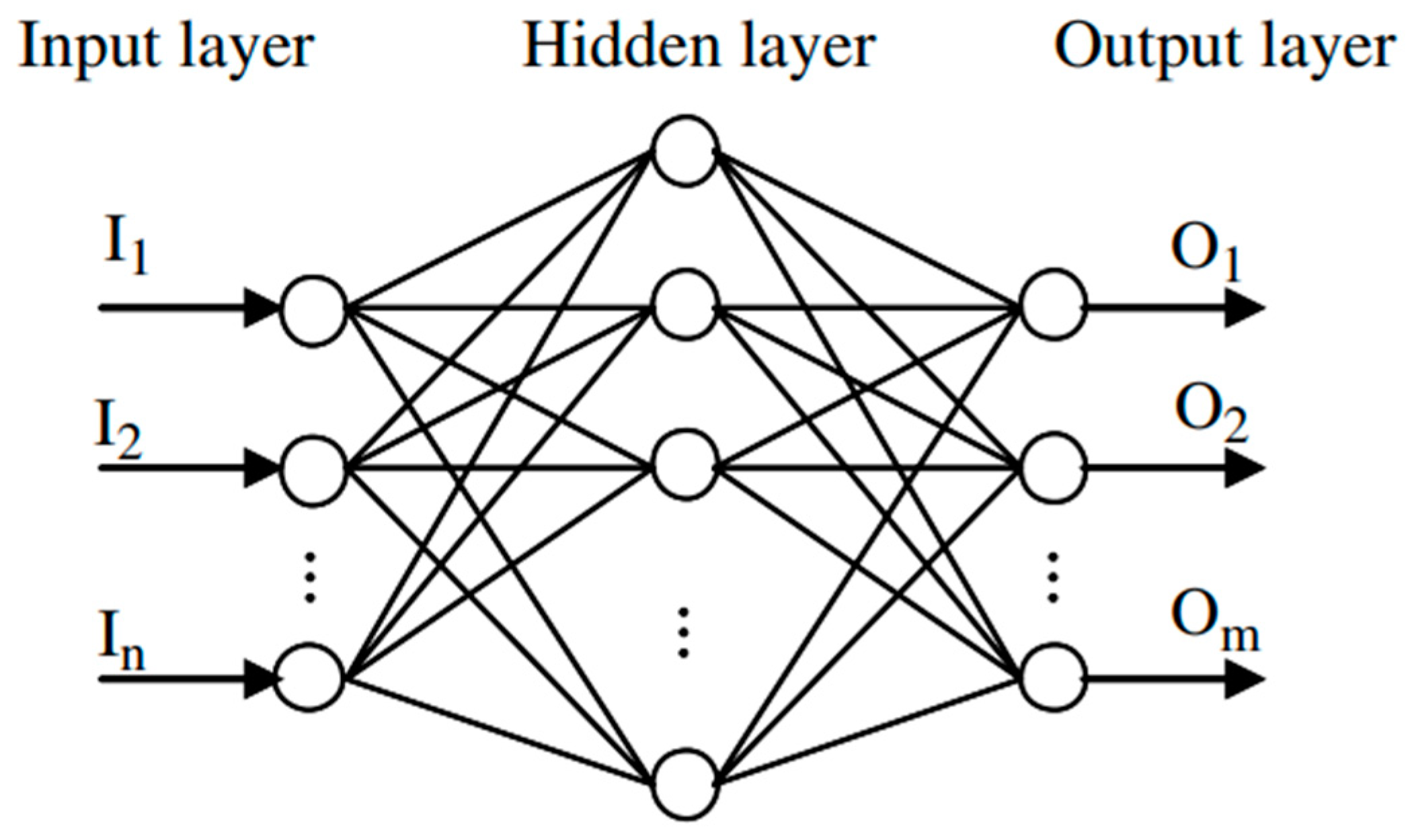
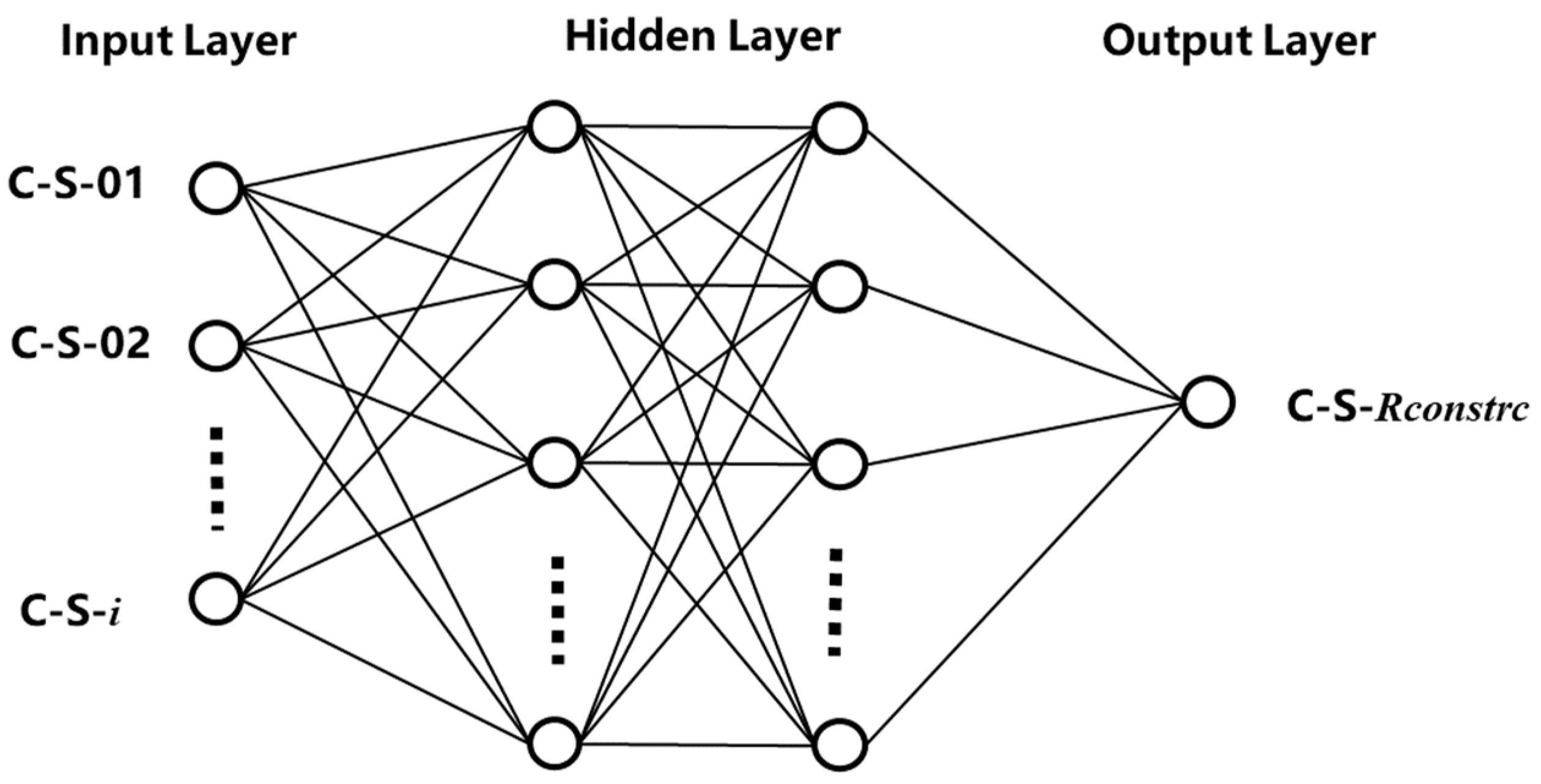
2.2. Application of the BP-ANN

Section 2.1. demonstrated that the target relationship is constant and time-invariant. Consequently, this study employed the BP-ANN [37] to model this relationship.

A neural network [37] is composed of an input layer, several hidden layers, and an output layer, interconnected through neurons. Each neuron in the network processes multiple inputs and generates an output signal via a transfer function, commonly referred to as an activation function. Connections between neurons are quantified by weights. The standard architecture of a neural network is depicted in Figure 2, featuring three distinct layers: the input layer (I), the hidden layer (H), and the output layer (O).

Specifically, each neuron in the hidden layer integrates an activation signal, which is the aggregate of all incoming inputs weighted accordingly [37], and subsequently generates an output via a transfer function:

$$x_j=\sum _i{I}_i{W}_{ij}$$

(16)

where $x_j$ denotes the activation signal at the j-th neuron in the hidden layer, $I_i$ is the input of the i-th neuron in the input layer, and $W_{ij}$ is the corresponding weight factor from $I_i$ to $x_j$. The neurons in the output layer receive the following activation signals from the hidden neurons [37]:

$$y_j=\sum _i{h}_i{W}_{jk}$$

(17)

where $h_i$ is the output of the j-th neuron in the hidden layer, $W_{jk}$ is the weight of the connection between the neurons j and k in the hidden and output layers, respectively, and $y_j$ denotes the input to the j-th neuron in the output layer. These inputs $y_j$ (j = 1, 2,…) are transformed again to give the outputs of the neural network [37]:

$$o_k={\displaystyle \frac{1}{1+e^{-y_k}}}$$

(18)

in which $o_k$ are predicted values of the network. The error function at the output neurons is defined as

$$\mathrm{E}\left(W\right)={\displaystyle \frac{1}{2}}\sum _k{\left(d_k-o_k\right)}^2$$

(19)

where $d_k$ and $o_k$ represent the desired and predicted values of the outputs, respectively. The error function should be minimized so that the neural network achieves the best performance.

Numerous algorithms have been crafted to reduce the error function E(W). The backpropagation (BP) algorithm stands out as the most prevalent, functioning as a supervised learning method. Within a BP neural network, the output layer’s error is retroactively disseminated through the hidden layer back to the input layer, aiming to refine the final output. The network’s weights are iteratively calculated and refined using the gradient descent approach to diminish the output error. Throughout the training phase, the network internalizes the correlations between system inputs and outputs via the interplay of connection weights.

This study adopted the foundational approach of the BP-ANN, as previously outlined in [37]. As depicted in Figure 3, responses measured at several cross-sections on the bridge served as inputs (i.e., $I_i$ in the input layer in Figure 2), and the response at a particular cross-section (i.e., $o_k$ illustrated in Equation (17)) constituted the output. The network is trained utilizing historical monitoring data. In this study, the BP-ANN was trained with data collected from field tests. Additional specifics on the BP-ANN configuration are provided in Section 4.2. It is important to note that the network inherently accounts for the potential impacts of unknown traffic conditions and air temperature on high-frequency responses, as these factors are encapsulated within the input–output mappings without any need for explicit adjustment.

The aforementioned derived physical characteristics do not modify the BP-ANN structure; they merely determine the selection of the proposed method and the necessity for the inputs and outputs of the network. Equation (10) demonstrated that, initially, the BP-ANN should be suitable for simulating the transfer matrix T without considering any time-related factors, despite the reconstruction of this study being for the purpose of predicting time-series signals. Moreover, once a network is trained to simulate the transfer matrix T, it should be applicable to various scenarios, including those with fluctuating temperature and traffic conditions. Additionally, this study did not delve into modifications or sophisticated algorithms for setting hyperparameters. Moreover, for certain typical prestressed bridges, the moment of inertia of the cross-section may vary along the length of the bridge due to the positioning of the prestressing cables, suggesting that the mode shape function would differ from that of equivalent non-prestressed bridges. Nevertheless, mode shape information was inherent and incorporated during the training process. As a result, the trained strain-related transfer matrix, which was obtained from monitoring data, differed in accordance with the arrangement of the prestressing cables. Upon completion of the bridge’s construction, both the mode shape function and the strain-related transfer function should be established, and they should remain time-independent and constant. Consequently, the proposed method should also be applicable for prestressed bridges.

Furthermore, as indicated from Equations (8a) and (8b) to (10), the mode shapes that form the output signal must be encompassed within those present in the input signal. Essentially, the mapping is the ratio of the mode coordinates across different cross-sections. For the data in the output neuron, if a mode shape’s modal coordinate is non-zero, corresponding to $-sin{\displaystyle \frac{n\pi x}{L}}$ in Equation (5b), one of the input features should also include the non-zero coordinate of that mode shape. Failing to do so would lead the neural network to attempt an orthogonal mapping between the input and output signals, which is assumed to be an erroneous mapping. For example, in the case of a simply supported beam, the modal coordinate of the second mode shape is zero. Calculating the mapping of the second mode coordinate between the mid-span and other cross-sections is problematic due to the transition from zero to non-zero values. To address this issue, it is recommended to analyze the frequency spectra of the high-frequency responses across all cross-sections. Randomly selecting inputs, meaning responses at arbitrary cross-sections, may not result in physically meaningful outcomes.

Additionally, for data processing, the high-frequency bridge responses were isolated from the raw monitoring data using a high-pass filter. For short-span bridges, with lengths around 30 m, the first natural vibrational frequency generally exceeds 3 Hz [38]. For bridges with spans ranging from 30 to 60 m, the primary bridge frequency consistently surpasses 2 Hz. In light of these considerations, the cutoff frequency for the high-pass filter in this study was established at 1 Hz.

3. Finite Element Simulation

This section introduces a series of finite element models to verify the physical characteristics derived for high-frequency bridge dynamics. To substantiate the hypothesis that the mapping of high-frequency responses across various sections remains time-independent and constant, a variety of scenarios were designed. These scenarios are differentiated by their traffic conditions, aiming to mimic the fluctuating traffic patterns encountered in real-world engineering contexts.

3.1. Finite Element Models

This study examined a numerical VBI system, featuring a simply supported beam and a quarter-vehicle model, as depicted in Figure 4. The design specifications for both the vehicle and the bridge followed the models utilized in prior research [35]. The beam exhibited a uniform cross-section, with the vehicle initially moving at a steady velocity of 5 m/s. Later, the speed was adjusted to simulate different traffic scenarios.

Table 1. Physical parameters of the vehicle.

Sprung mass (kg)	1200
Spring stiffness (N/m)	500,000
Bouncing frequency (Hz)	3.25

and

Table 2. Physical parameters of the beam.

Mass per meter (kg/m)	4800
EI (N/m2)	3.33 × 109
First bending frequency (Hz)	2.08
Second bending frequency (Hz)	8.33
Length (m)	25

detail the respective physical parameters of the vehicle and the bridge.

The VBI system was modeled using the commercial software ABAQUS 2020 [39], as illustrated in Figure 4, employing a three-dimensional approach. Both the bridge and the quarter-vehicle were represented with solid elements. The quarter-vehicle model comprises a sprung mass and a wheel, both of which were also modeled using solid elements. These components are linked by a spring element. The wheel is shaped as a cylinder, matching the width of the beam’s cross-section. This study excluded road roughness from its considerations, given its minimal impact on the bridge responses [40]. The interaction between the wheel and the beam surfaces was captured using the penalty method. The dynamic responses of the system were computed using the Hilber–Hughes–Taylor (HHT) algorithm with a 0.01 s time step. The accuracy of this simulation methodology was confirmed in prior studies. Further details on the simulation process can be referred to in the previous research [41].

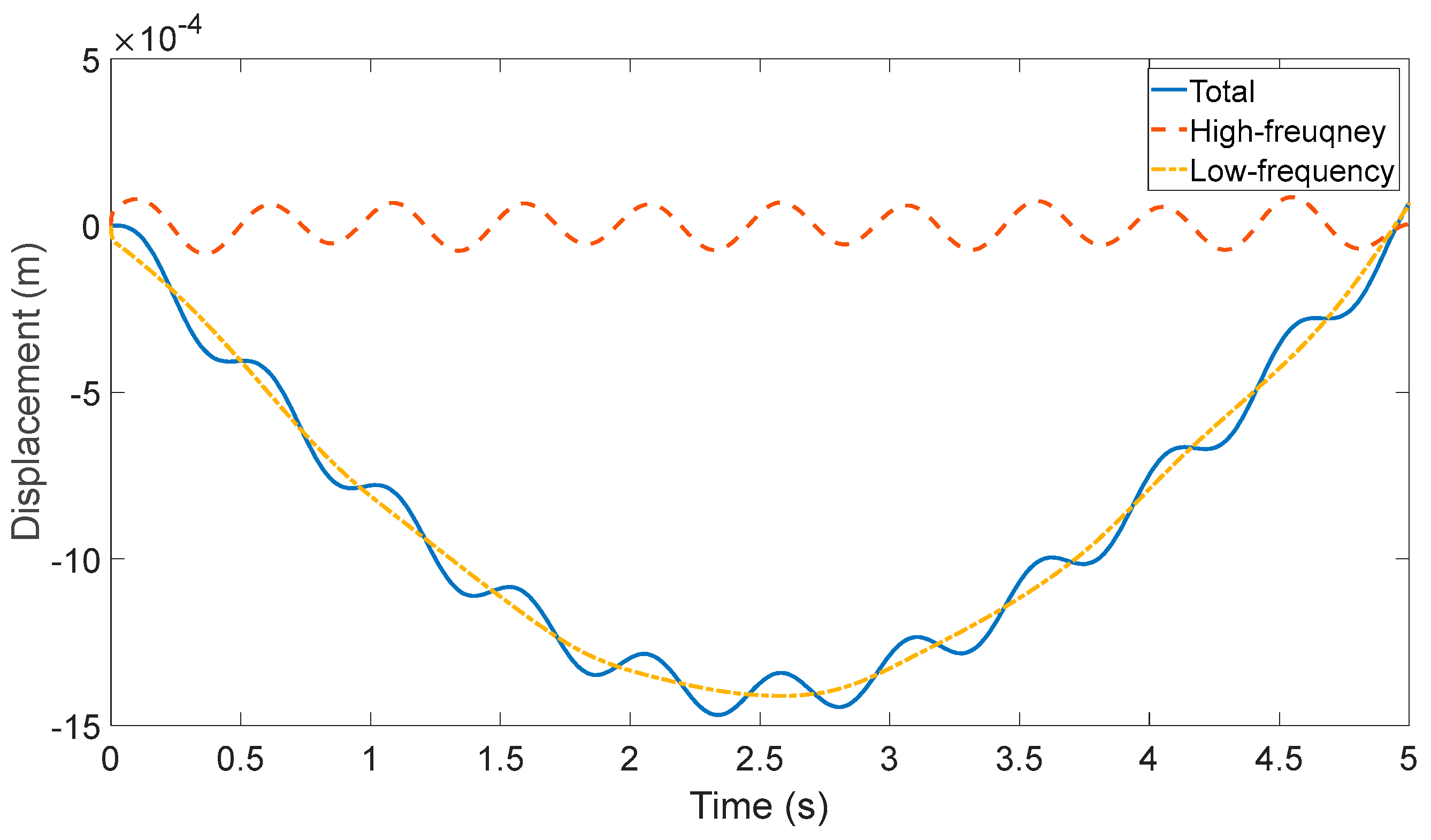
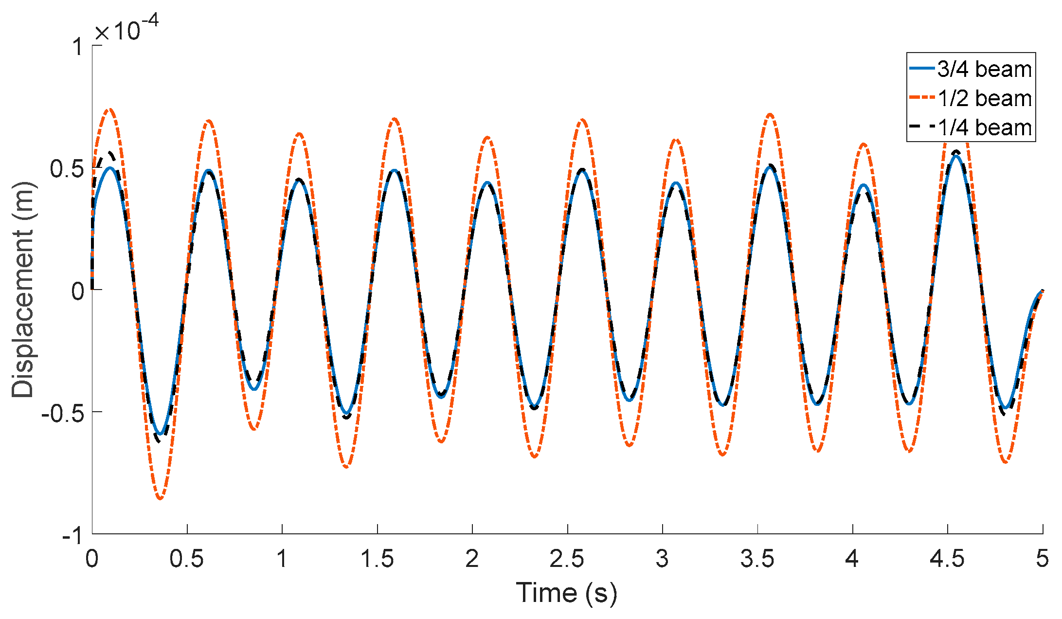
3.2. Physical Characteristics of High-Frequency Bridge Responses

Figure 5 displays the time history of the vertical displacement at the mid-span of the beam. To eliminate the low-frequency components, a high-pass filter [42] set at a frequency of 1 Hz was applied. The filtered high-frequency and the low-frequency bridge displacements are both depicted in Figure 5.

This study examined the physical characteristics of a high-frequency bridge’s dynamic responses. The high-frequency bridge displacement manifested as a periodic sinusoidal waveform, which coincided with the theoretical formulation presented in Equation (5b). Furthermore, the low-frequency displacement predominantly contributed to the total displacement, aligning with Biggs’ findings [43]. Conversely, the amplitude of the high-frequency bridge displacement was significantly smaller, a result that is consistent with the research conducted by He and Zhu [44].

Utilizing a band-pass filter that spanned the range of 1 Hz to 5 Hz, the high-frequency bridge vibrations corresponding to the first natural frequency at the 3/4 beam and mid-span, as well as the 1/4 beam, were isolated and are depicted in Figure 6. The illustration demonstrates that these three points vibrate in unison and in phase for single-frequency vibration, a phenomenon that aligns with Equation (5b). Additionally, it is posited that each high-frequency vibrational mode induces simultaneous, in-phase vibrations at different beam locations, with the sole variation being the mode shape coordinate, as per Equation (5b).

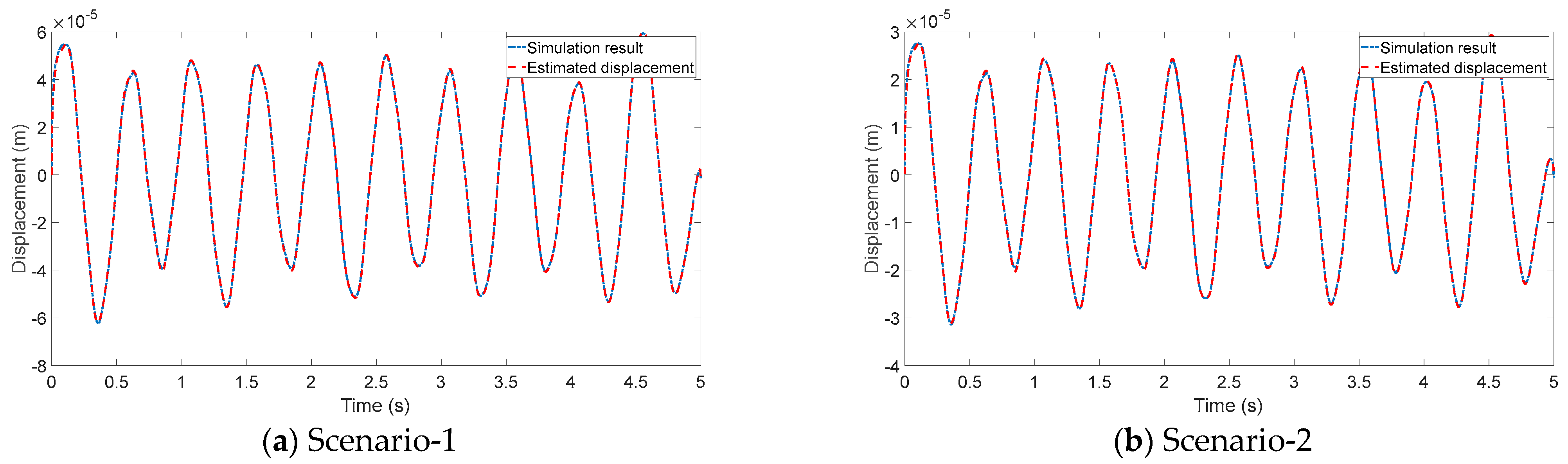
3.3. Validation of the Time-Invariant Relationship

The constant time-invariant relationship was demonstrated through a series of validations, each of which employed a different scenario. In these scenarios, the traffic condition was adjusted to reflect changes in vehicle status, speed, and volume. These parameters encapsulate the most prevalent time-dependent variables in the context of fluctuating traffic conditions. Should a mapping relationship, whether built upon the responses from a single scenario or deduced theoretically, be capable of encapsulating the relationships across all scenarios, it would be reasonable to deduce that the target relationship is indeed time-invariant and constant for a given bridge. The specifics of these scenarios are the following:

(1)

Scenario-1—The above finite element model with a simply supported beam and quarter-vehicle;

(2)

Scenario-2—A vehicle with a different frequency and half the mass of Scenario-1 to simulate a different mass and a different bouncing frequency of the vehicle;

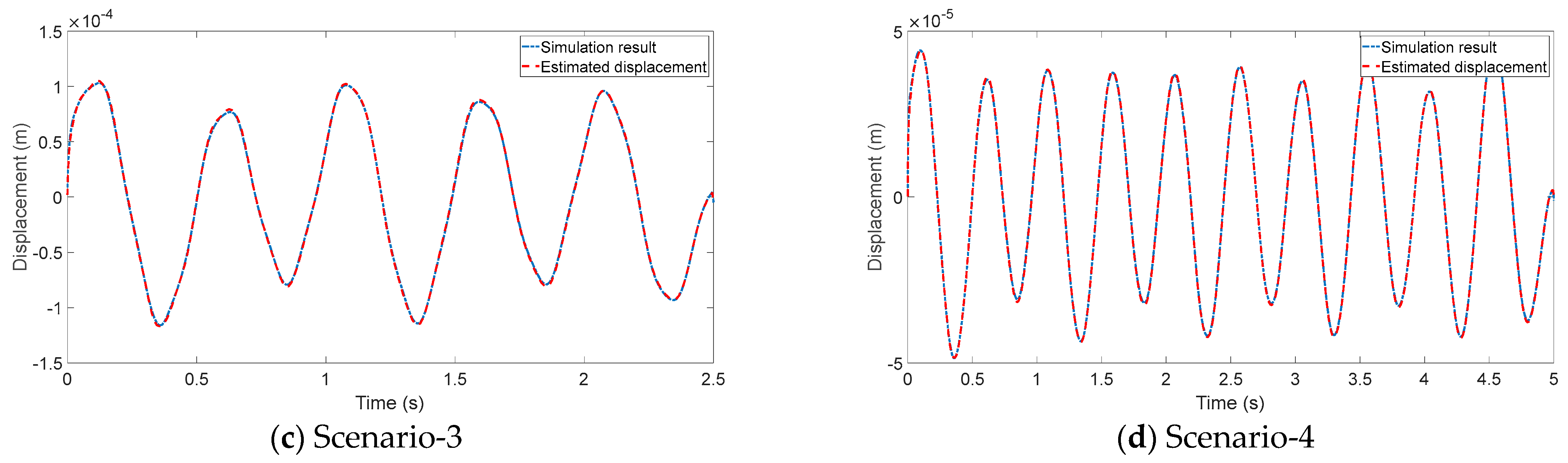
(3)

Scenario-3—A vehicle with different speed (the vehicle’s speed in this scenario was twice that of Scenario-1 (10 m/s));

(4)

Scenario-4—Simultaneous vehicle traffic, whereby two vehicles traverse the beam, moving in opposite directions, and the first vehicle mirrors the physical attributes and velocity of the vehicle featured in Scenario-1, whereas the second vehicle possesses half the mass and progresses at a reduced speed of 3 m/s.

To reconstruct the responses at 1/4 beam, dynamic responses at 3/4 beam and mid-beam were used. The transfer matrix from $x_{3/4}$ and $x_{1/2}$ to $x_{1/2}$ and $x_{1/4}$ was calculated using Equations (8a), (8b), (9) and (10). Figure 7 illustrates the reconstruction results for these four scenarios. The reconstructed beam responses matched well with the simulation results, substantiating that the relationship between sections was indeed time-invariant and constant, irrespective of differing traffic conditions. Additionally, it was supposed that changes in temperature would not affect the mode shape, and thus, the derived transfer matrix should be applicable under varying temperature conditions.

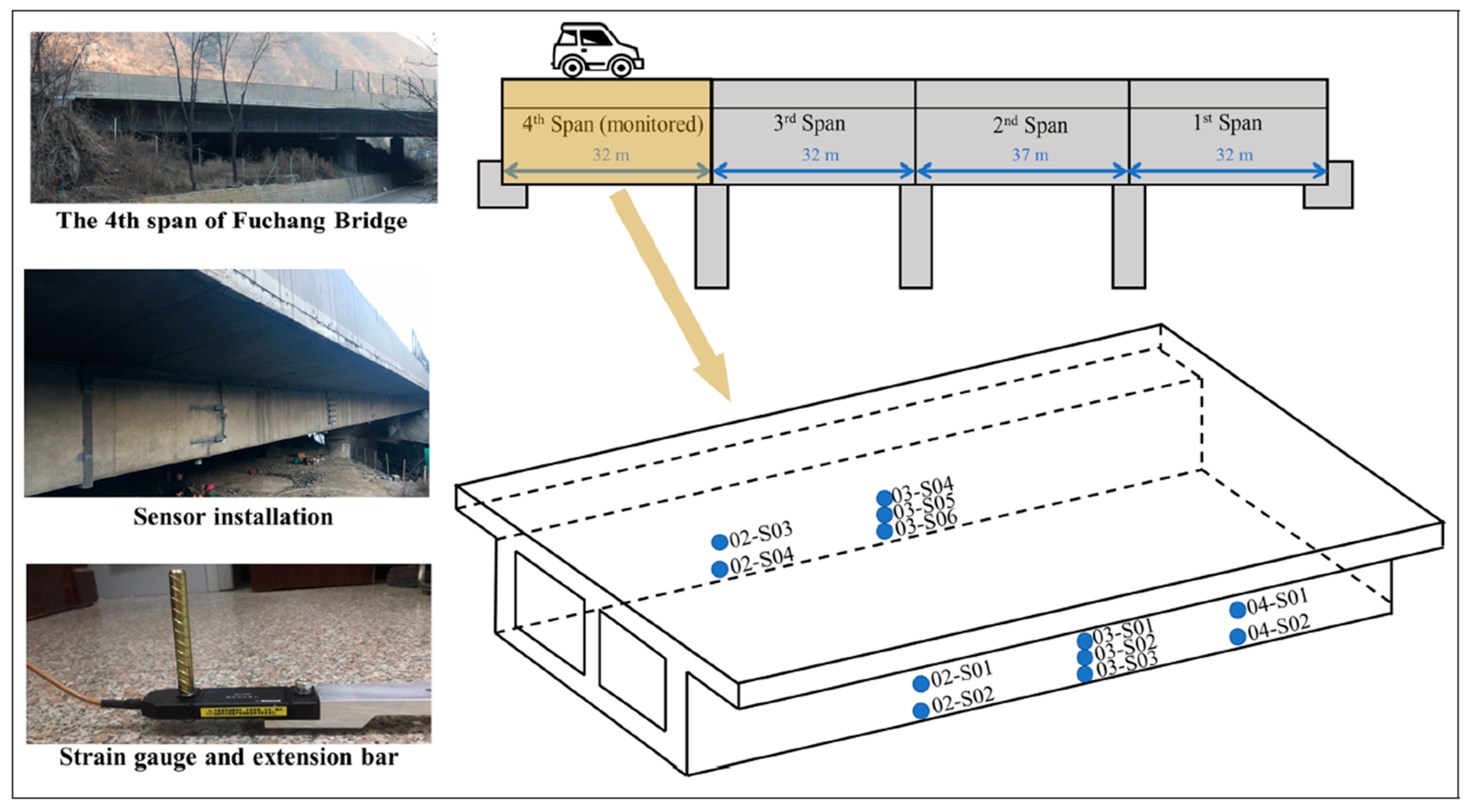
4. Response Reconstruction for an Actual Continuous Bridge

In this section, the proposed method was validated with monitoring data from an actual continuous concrete bridge. Firstly, an overview of the monitoring system and the bridge is provided. Following this, the architecture of the BP-ANN for response reconstruction is detailed. Finally, the method’s effectiveness was confirmed through two case studies which accounted for varying temperature and traffic conditions.

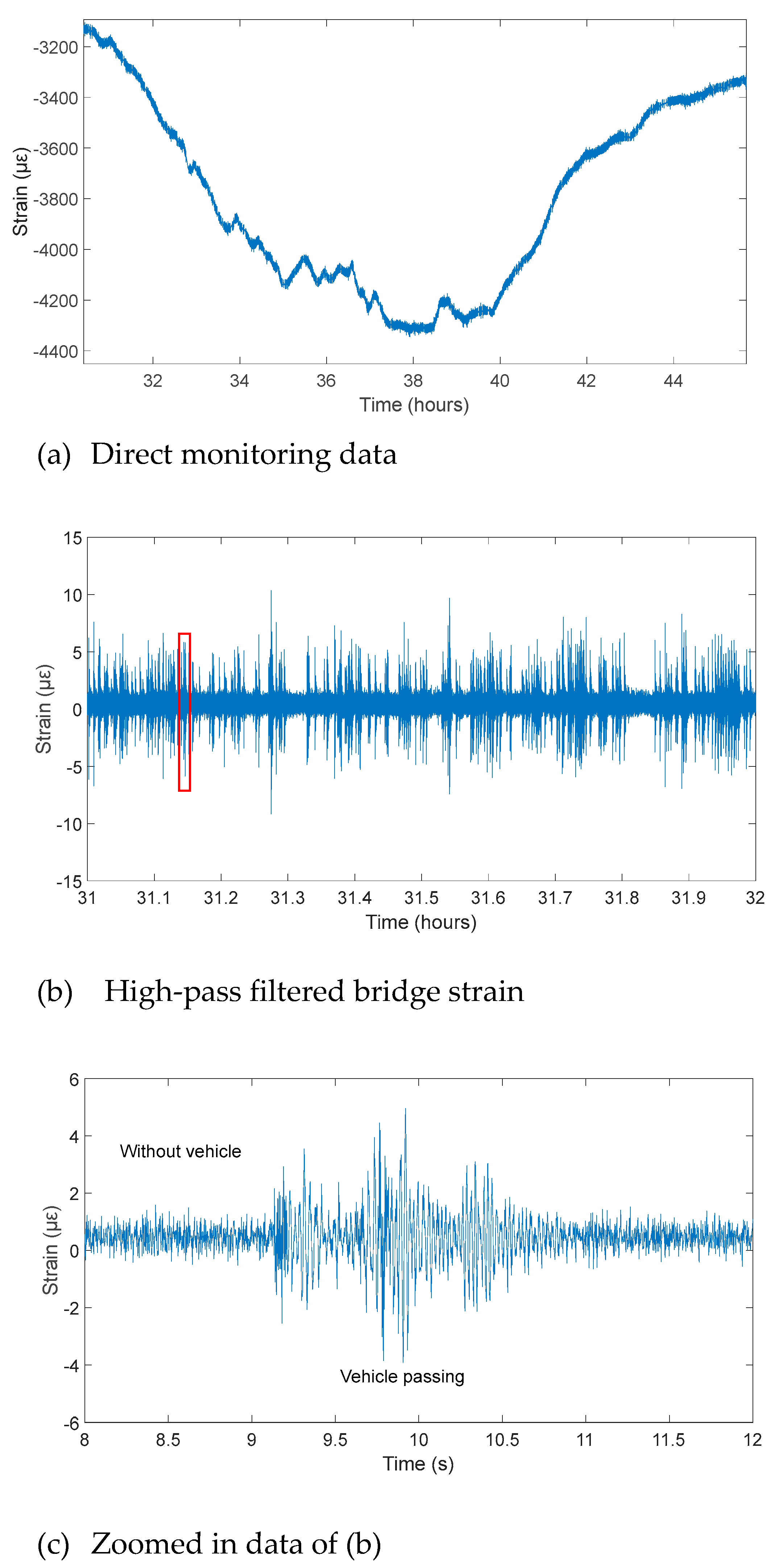
4.1. Information on the Continuous Bridge and Monitoring System

The Fuchang Bridge, located in Hebei Province, China, comprises two distinct dual bridges on the left and right sides, supported by rubber bearings. Both of these bridges are typical, prestressed, concrete, continuous beam bridges. The left-side bridge is a prestressed continuous box-girder bridge comprising four continuous spans (32 m + 32 m + 37 m + 32 m), totaling 133 m in length, as illustrated in Figure 8 [45]. The right-side bridge, measuring 187.2 m in length, is composed of two separate structures: one is a prefabricated, prestressed, concrete, continuous T-beam bridge, and the other is a prestressed, continuous box-girder bridge. A health monitoring system was installed on the fourth span of the left-side bridge, with twelve strain gauges placed at three cross-sections (02, 03, and 04). The strain data were sampled at a frequency of 50 Hz during the monitoring period from March 2018 to December 2018.

4.2. Data Preparation and ANN Configuration

Figure 9 presents a sample of the typical monitoring data covering several hours. The primary cause of strain variation was temperature-induced strain, as shown in Figure 9a. The local peaks observed in the strain time–history curve were induced by the passage of vehicles. It is crucial to highlight that these local peaks represent the effect of both low-frequency and high-frequency bridge strain. Figure 9b depicts the high-pass filtered bridge strain, which is a zero-mean time series. Considering the bridge’s natural frequencies were above 1 Hz, the cutoff frequency was set at 1 Hz. Figure 9c offers an enlarged view of the filtered data presented in Figure 9b.

It should be noted that this study did not record either traffic conditions or environmental effects. However, traffic conditions (with/without a vehicle, single/multiple vehicles) could be inferred from the amplitude and duration of the high-frequency bridge responses. For instance, the data in Figure 9c were categorized into “Vehicle passing” and “Without vehicle”. The high-frequency responses caused by vehicles exhibited a significantly higher amplitude. Additionally, the duration of these high-amplitude responses aided in distinguishing between the effects of a single vehicle and those of multiple vehicles. The average velocity for vehicles on this bridge was between 40 and 70 km/h, translating to a passage time of roughly 4 to 9 s per vehicle. If the high amplitude persisted beyond this typical time frame, this suggested that several vehicles were crossing the bridge at the same time. During the validation process, it was verified that both the training and test data encompassed scenarios involving both single and multiple vehicles.

The dynamic responses at one cross-section were predicted using monitoring data from two other cross-sections. For each cross-section, a single strain gauge was chosen, yielding two input features for the BP-ANN and one output feature. The BP-ANN architecture included two hidden layers: the first with 128 neurons and the second with 32 neurons. The learning rate was configured at 0.001, with a batch size of 100 and a total of 500 epochs. The rectified linear unit (ReLU) function is used as the activation function. Since the theoretical derivation showed that the relationship was time-invariant, during training, data from various time points were randomly sampled in batches.

4.3. Data Analysis

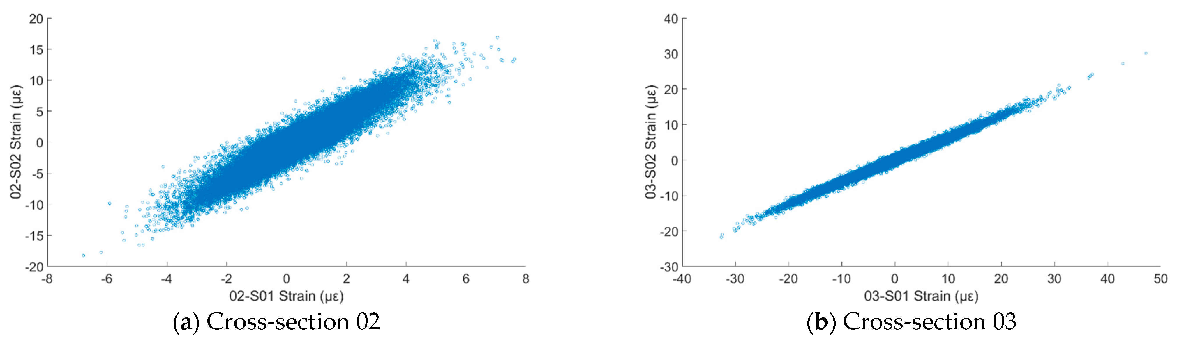
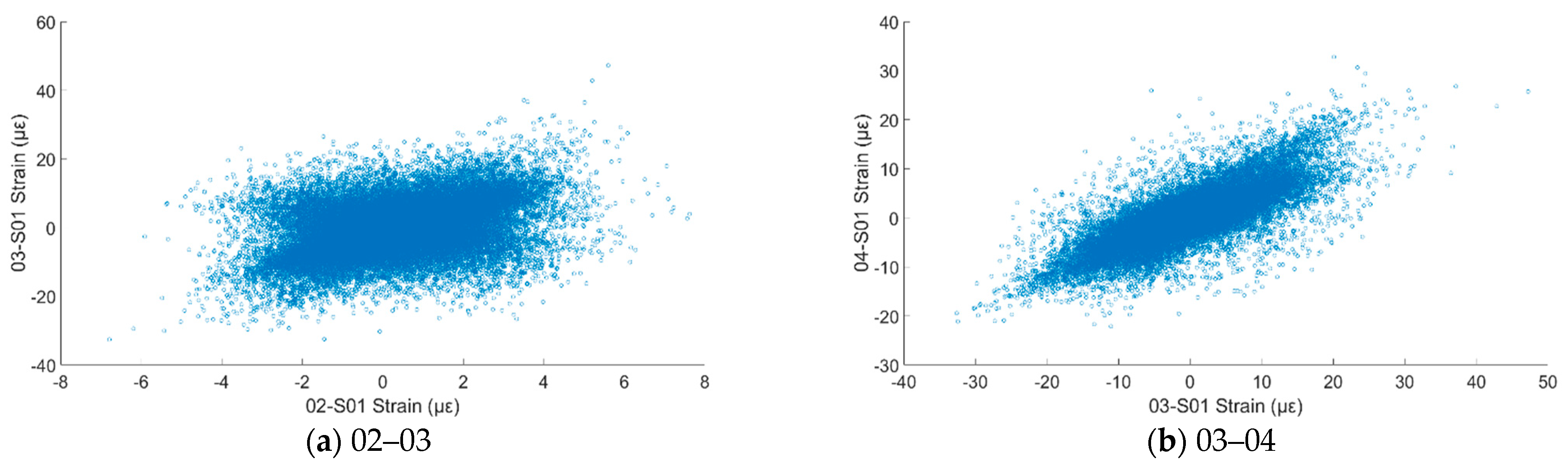
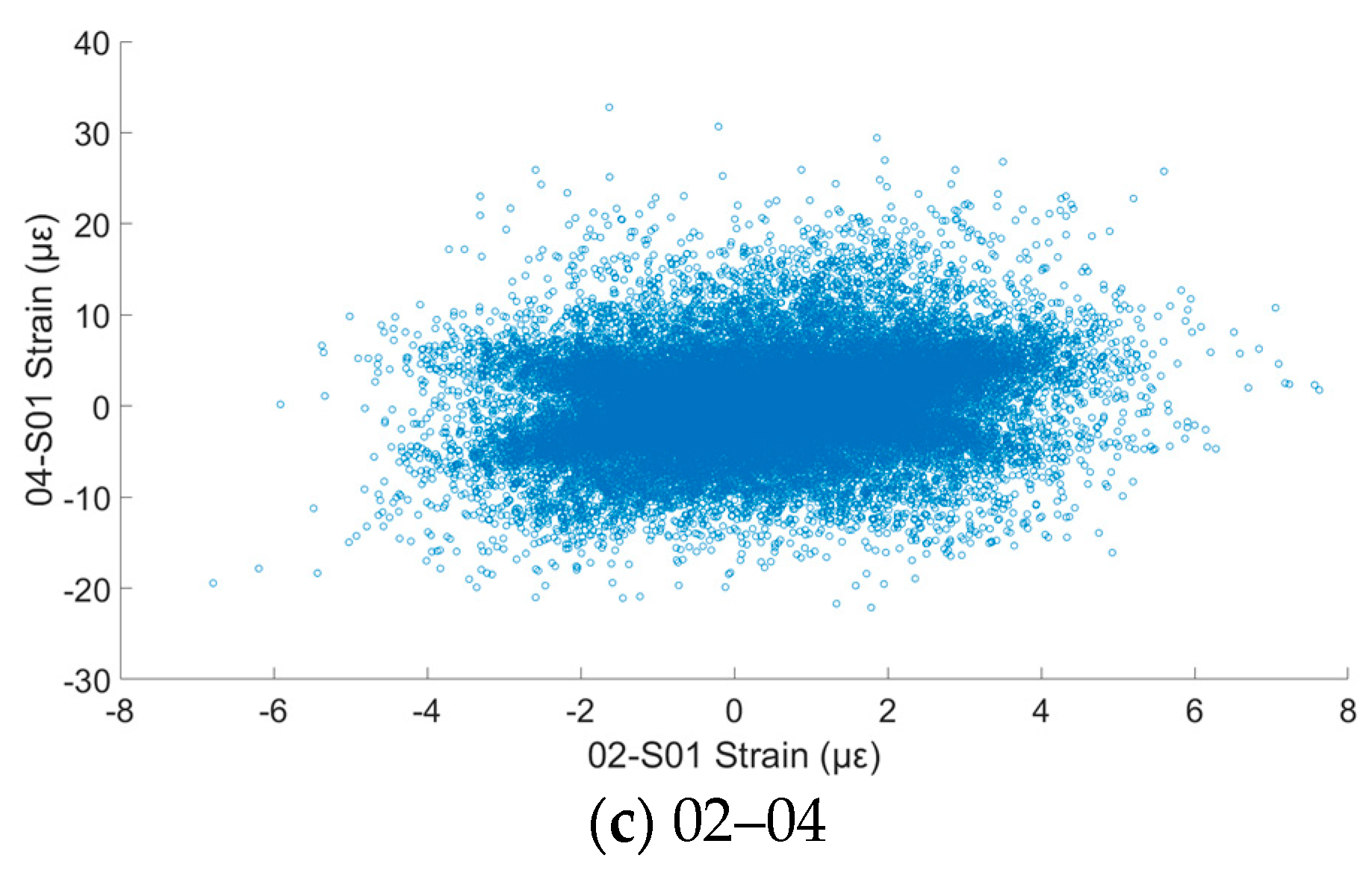
4.3.1. Intersectional Relationship between High-Frequency Responses

Initially, this study focused on exploring the potential correlation between the high-frequency responses of strain gauges within a single cross-section and across multiple cross-sections. Figure 10 displays the scatter plot of the high-frequency responses between 02-S01 and 02-S02, demonstrating a linear relationship between these two gauges. This linearity can be attributed to the strain being proportional to the distance of the gauge from the vertical axis line within the same cross-section. Furthermore, Equation (14) confirms that this linear relationship holds true for all bending modes.

In consideration of the high-frequency responses observed across different cross-sections, it was evident that the linear relationship that was previously discussed was not an appropriate fit. Figure 11a–c illustrate scatter plots between strain gauges 02-S01, 03-S01, and 04-S01, respectively. Compared to the pattern shown in Figure 10, identifying the intersectional relationship between strains at different cross-sections is more complex. According to Equation (5b), it was hypothesized that the high-frequency responses were composed of multiple modes, each with its own specific modal coordinates. These coordinates differed across these cross-sections. As a result, the responses at these cross-sections did not necessarily align with a linear relationship.

4.3.2. Case Configuration

To validate the proposed method, monitoring data from two non-consecutive days, one in August and the other in October, were utilized for analysis. The temperature profiles for these days were distinct and did not overlap. For each day, a 30 min monitoring period was chosen for examination. As previously mentioned, the traffic conditions were not specified, and time-variant factors such as traffic and temperature were not set as input information for the training of the BP-ANN. The validation was conducted through two designed cases, as detailed below.

Case-1: Validation of the proposed method was conducted using monitoring data from August. A BP-ANN was constructed using the monitoring record. The data were partitioned, with 20% allocated for network training and the remaining 80% dedicated to verifying the model’s predictive accuracy. To reconstruct the strain readings at location 04-S01, input data from strain gauges 02-S01 and 03-S01 were used.

Case-2: In the second case, a new series of data was generated by merging the monitoring data from both August and October. Following this, a new BP-ANN was trained. A total of 33% of the monitoring data were employed for training purposes. Specifically, the 20 min monitoring data from August were used to develop the neural network, and the remaining 40 min of data, combined monitoring data from both August and October, were then used to evaluate the accuracy of the developed network.

As previously stated in Section 2.1, once a transfer matrix has been successfully simulated using a BP-ANN, it becomes suitable for long-term monitoring applications, even if it was initially derived from short-term monitoring data. Accordingly, in Cases 1 and 2, the duration of the test data was designed to exceed the length of the data employed in the construction of the BP-ANN. In Case 2, a transfer matrix was established using less than 1% of the total data, proving its applicability throughout the entire monitoring period, spanning from August to October. Moreover, the exact traffic conditions and temperatures remained unknown and were unlikely to be identical in both the training and test datasets. This setup aimed to confirm that the BP-ANN’s performance remained consistent and was not affected by the variability in traffic conditions and temperature fluctuations.

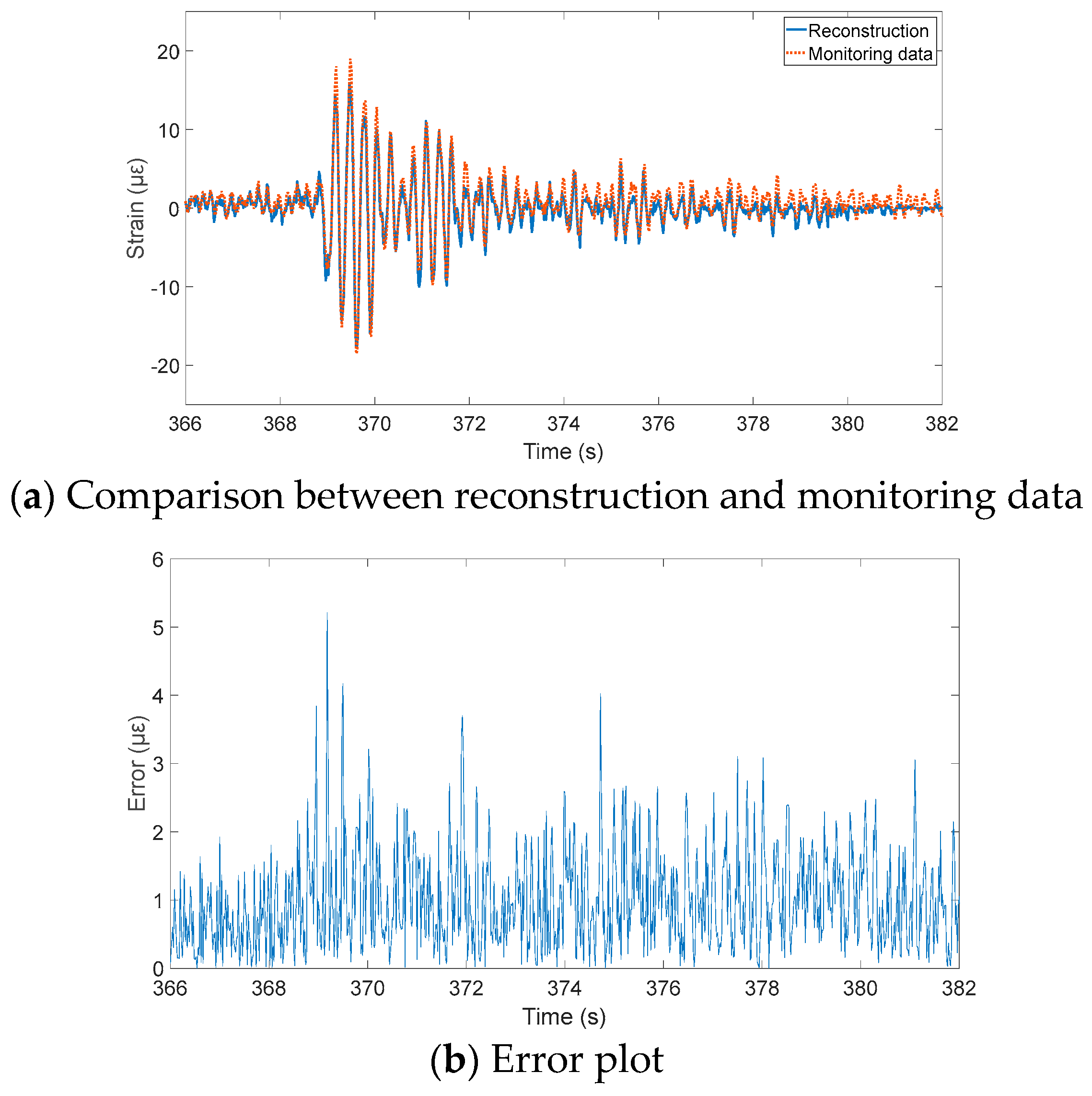
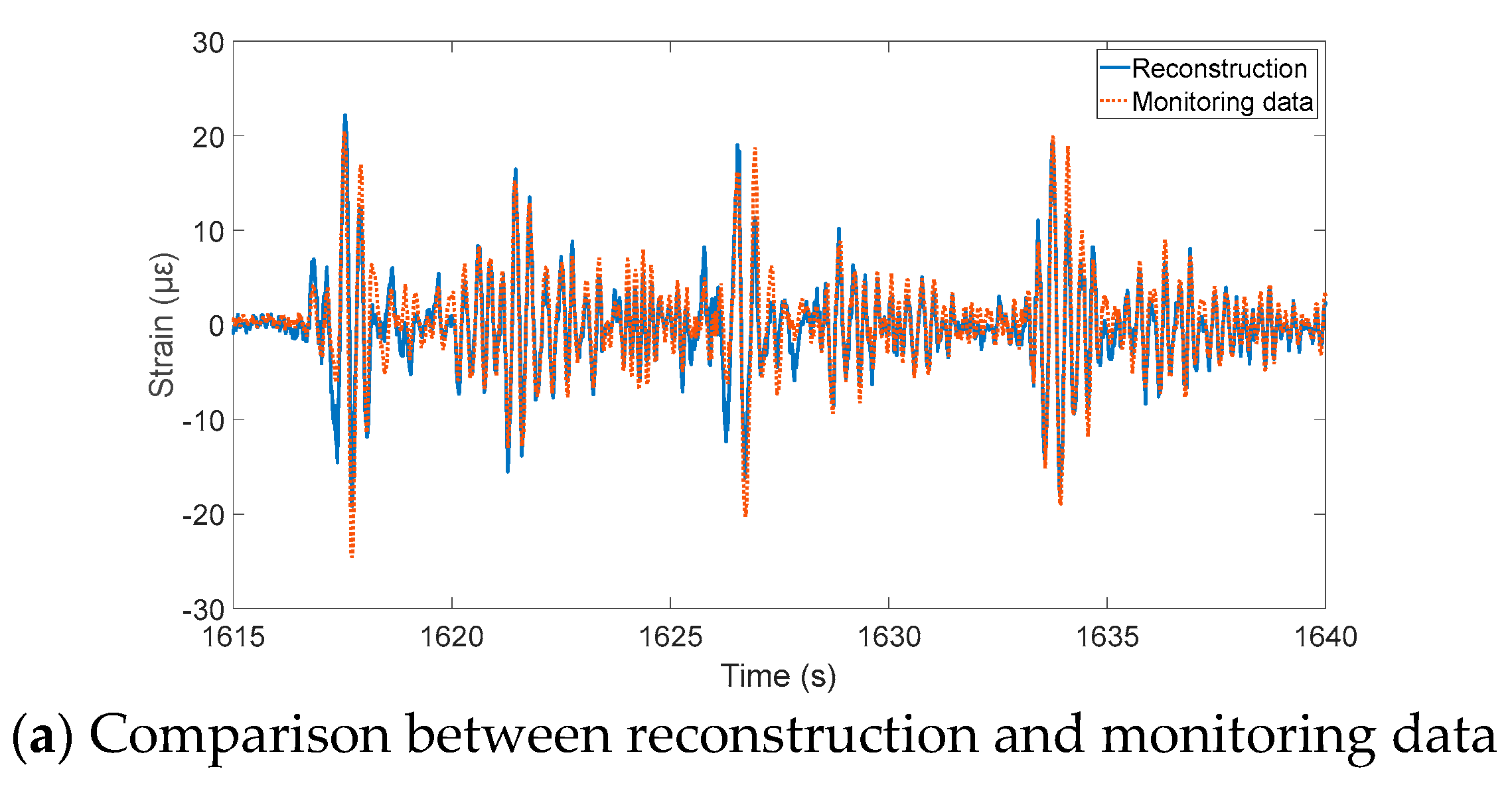
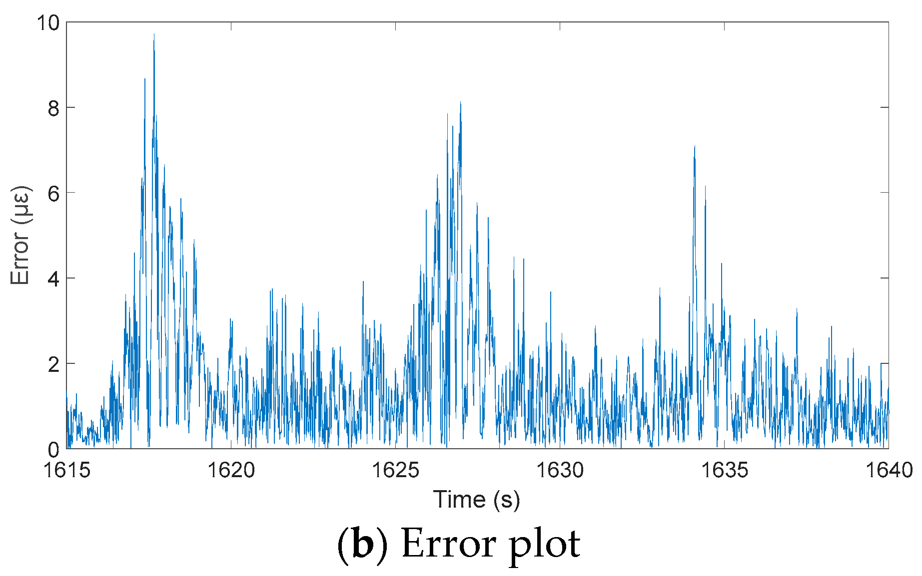
4.3.3. Result Analysis

Figure 12a presents the reconstruction outcome for Case-1. The strain data reconstructed at 04-S01 closely aligned with the actual high-frequency bridge strain observed through monitoring. Furthermore, Figure 12b illustrates the time history of the reconstruction error, indicating that the discrepancies between the reconstructed results and the monitoring data were relatively minor throughout the entire monitoring time frame.

Figure 13 shows the reconstruction result of Case-2. The reconstruction result aligned well with the monitoring data. Moreover, the reconstruction outcome reflected a scenario with multiple vehicles, indicating that the simulated relationship was applicable under random traffic conditions involving several vehicles. This further supported the notion that the relationship between the variables remained time-invariant and constant, regardless of fluctuating traffic conditions. Additionally, considering that the input training data were constrained to only 20 min, the validation in Case-2 underscores that the proposed method was viable for practical engineering applications, enabling the use of short-term monitoring data for the reconstruction of long-term data.

Additionally, this study endeavored to delve into the reconstruction of torsion modes as part of future research. Figure 14 offers a visual comparison of strain data across different sides of S02. In deviation from the linear relationship depicted in Figure 10, the strains measured on opposing sides did not maintain a linear correlation. This finding implies that torsion modes require consideration in the analysis. Nonetheless, subsequent evaluations revealed that the existing strain gauge configuration in the field experiment was not adequate to capture torsion modes. This issue will be discussed in a future study.

5. Conclusions

The objective of this study was to reconstruct high-frequency bridge vibrations across different bridge cross-sections. The theoretical responses of a bridge in a simple VBI system were initially analyzed. The relationship between sections was then explicitly formulated to discuss its time-invariant characteristics under varying temperature and traffic conditions. Subsequently, a BP-ANN network was chosen for reconstructing the high-frequency bridge responses, leveraging these derived characteristics. A series of finite element models were developed to verify these characteristics. A field experiment was conducted on a continuous bridge to validate the proposed method. The main conclusions are summarized below as the following:

(1)

Essentially, this relationship can be characterized as a transfer matrix that is associated with mode shapes. The target relationship should remain constant and time-invariant under varying traffic and temperature conditions.

(2)

The BP-ANN method proved to be an effective tool for reconstructing responses across various cross-sections. In the field test, the reconstruction result matched well with the monitoring data.

(3)

The proposed method facilitated the utilization of relatively short-term monitoring data to reconstruct long-term bridge responses effectively.

In comparison to the preceding study, the proposed method is data-driven and does not necessitate the construction of finite element models, thereby enhancing its time efficiency for engineering applications. Moreover, this method permits long-term monitoring with a short-term monitoring database, thus obviating the necessity for a vast database and making it more accessible for implementation in real-world engineering scenarios. Furthermore, grounded in the bridge’s physical characteristics, it is expected to be applicable to general short- and medium-span bridges.

It is important to note that the current study only considered bending modes, and not torsional modes, which may also contribute to the bridge dynamics in bridges with multiple lanes. As a result, the current method might not encompass all critical vibrational modes. It is suggested that sensor placement be optimized accordingly. Moreover, this study was limited to bridges with constant mode shapes. However, the method may not be suitable for simulating relationships in some large-span bridges that exhibit non-linear time-dependent properties or have non-linear material components whose mode shapes may change over time. These concerns will be addressed in future studies.

References

1. Sun, L.; Li, Y.; Zhu, W.; Zhang, W. Structural Response Reconstruction in Physical Coordinate from Deficient Measurements. Eng. Struct. 2020, 212, 110484. [Google Scholar] [CrossRef]
2. Lu, Y.; Tang, L.; Chen, C.; Zhou, L.; Liu, Z.; Liu, Y.; Jiang, Z.; Yang, B. Reconstruction of Structural Long-Term Acceleration Response Based on BiLSTM Networks. Eng. Struct. 2023, 285, 116000. [Google Scholar] [CrossRef]
3. Almutairi, M.; Nikitas, N.; Abdeljaber, O.; Avci, O.; Bocian, M. A Methodological Approach towards Evaluating Structural Damage Severity Using 1D CNNs. Structures 2021, 34, 4435–4446. [Google Scholar] [CrossRef]
4. Zhang, S.; Wang, Z.; Jian, Z.; Liu, G.; Liu, X. A Two-Step Method for Beam Bridge Damage Identification Based on Strain Response Reconstruction and Statistical Theory. Meas. Sci. Technol. 2020, 31, 075008. [Google Scholar] [CrossRef]
5. Ni, P.; Han, Q.; Du, X.; Cheng, X. Bayesian Model Updating of Civil Structures with Likelihood-Free Inference Approach and Response Reconstruction Technique. Mech. Syst. Signal Process. 2022, 164, 108204. [Google Scholar] [CrossRef]
6. Deng, L.; Cai, C.S. Bridge Model Updating Using Response Surface Method and Genetic Algorithm. J. Bridge Eng. 2010, 15, 553–564. [Google Scholar] [CrossRef]
7. Altunişik Ahmet, C.; Kalkan, E.; Okur Fatih, Y.; Olguhan Şevket, K.; Korhan, O. Finite-Element Model Updating and Dynamic Responses of Reconstructed Historical Timber Bridges using Ambient Vibration Test Results. J. Perform. Constr. Facil. 2020, 34, 04019085. [Google Scholar] [CrossRef]
8. Jiang, K.; Han, Q.; Du, X.; Ni, P. Structural Dynamic Response Reconstruction and Virtual Sensing Using a Sequence to Sequence Modeling with Attention Mechanism. Autom. Constr. 2021, 131, 103895. [Google Scholar] [CrossRef]
9. Lei, X.; Siringoringo, D.M.; Sun, Z.; Fujino, Y. Displacement Response Estimation of a Cable-Stayed Bridge Subjected to Various Loading Conditions with One-Dimensional Residual Convolutional Autoencoder Method. Struct. Health Monit. 2023, 22, 1790–1806. [Google Scholar] [CrossRef]
10. Overschee, P.; Moor, B. Subspace Identification for Linear Systems: Theory—Implementation—Applications; Springer: Norwell, MA, USA, 1996; Volume 1. [Google Scholar]
11. Peeters, B.; De Roeck, G. Reference-based stochastic subspace identification for output-only modal analysis. Mech. Syst. Signal Process. 1999, 13, 855–878. [Google Scholar] [CrossRef]
12. Yang, X.-M.; Yi, T.-H.; Qu, C.-X.; Li, H.-N.; Liu, H. Automated eigensystem realization algorithm for operational modal identification of bridge structures. J. Aerosp. Eng. 2019, 32, 04018148. [Google Scholar] [CrossRef]
13. Zhang, G.; Ma, J.; Chen, Z.; Wang, R. Automated Eigensystem Realisation Algorithm for Operational Modal Analysis. J. Sound Vib. 2014, 333, 3550–3563. [Google Scholar] [CrossRef]
14. Hossain, M.S.; Ong, Z.C.; Ismail, Z.; Noroozi, S.; Khoo, S.Y. Artificial Neural Networks for Vibration Based Inverse Parametric Identifications: A Review. Appl. Soft Comput. 2017, 52, 203–219. [Google Scholar] [CrossRef]
15. Xin, J.; Zhou, C.; Jiang, Y.; Tang, Q.; Yang, X.; Zhou, J. A Signal Recovery Method for Bridge Monitoring System Using TVFEMD and Encoder-Decoder Aided LSTM. Measurement 2023, 214, 112797. [Google Scholar] [CrossRef]
16. Oh, B.K.; Glisic, B.; Kim, Y.; Park, H.S. Convolutional Neural Network–Based Data Recovery Method for Structural Health Monitoring. Struct. Health Monit. 2020, 19, 1821–1838. [Google Scholar] [CrossRef]
17. Zhang, H.; Xu, C.; Jiang, J.; Shu, J.; Sun, L.; Zhang, Z. A Data-Driven Based Response Reconstruction Method of Plate Structure with Conditional Generative Adversarial Network. Sensors 2023, 23, 6750. [Google Scholar] [CrossRef] [PubMed]
18. Zhang, R.; Meng, L.; Mao, Z.; Sun, H. Spatiotemporal Deep Learning for Bridge Response Forecasting. J. Struct. Eng. 2021, 147, 04021070. [Google Scholar] [CrossRef]
19. Tian, Y.; Xu, Y.; Zhang, D.; Li, H. Relationship Modeling between Vehicle-induced Girder Vertical Deflection and Cable Tension by BiLSTM Using Field Monitoring Data of a Cable-stayed Bridge. Struct. Control Health Monit. 2021, 28, e2667. [Google Scholar] [CrossRef]
20. Ni, P.; Li, Y.; Sun, L.; Wang, A. Traffic-Induced Bridge Displacement Reconstruction Using a Physics-Informed Convolutional Neural Network. Comput. Struct. 2022, 271, 106863. [Google Scholar] [CrossRef]
21. Oh, B.K.; Kim, J. Optimal Architecture of a Convolutional Neural Network to Estimate Structural Responses for Safety Evaluation of the Structures. Measurement 2021, 177, 109313. [Google Scholar] [CrossRef]
22. Oh, B.K.; Park, H.S.; Glisic, B. Prediction of Long-Term Strain in Concrete Structure Using Convolutional Neural Networks, Air Temperature and Time Stamp of Measurements. Autom. Constr. 2021, 126, 103665. [Google Scholar] [CrossRef]
23. Jiang, H.; Wan, C.; Yang, K.; Ding, Y.; Xue, S. Continuous Missing Data Imputation with Incomplete Dataset by Generative Adversarial Networks–Based Unsupervised Learning for Long-Term Bridge Health Monitoring. Struct. Health Monit. 2022, 21, 1093–1109. [Google Scholar] [CrossRef]
24. Fan, G.; He, Z.; Li, J. Structural Dynamic Response Reconstruction Using Self-Attention Enhanced Generative Adversarial Networks. Eng. Struct. 2023, 276, 115334. [Google Scholar] [CrossRef]
25. Zhuang, Y.; Qin, J.; Chen, B.; Dong, C.; Xue, C.; Easa, S.M. Data Loss Reconstruction Method for a Bridge Weigh-in-Motion System Using Generative Adversarial Networks. Sensors 2022, 22, 858. [Google Scholar] [CrossRef] [PubMed]
26. Hwang, D.; Kim, S.; Kim, H.K. Long-Term Damping Characteristics of Twin Cable-Stayed Bridge under Environmental and Operational Variations. J. Bridge Eng. 2021, 26, 04021062. [Google Scholar] [CrossRef]
27. Bocian, M.; Nikitas, N.; Kalybek, M.; Kużawa, M.; Hawryszków, P.; Bień, J.; Onysyk, J.; Biliszczuk, J. Dynamic Performance Verification of the Rędziński Bridge Using Portable Camera-Based Vibration Monitoring Systems. Archiv. Civ. Mech. Eng. 2022, 23, 40. [Google Scholar] [CrossRef]
28. Nikitas, N.; Macdonald, J.H.; Jakobsen, J.B. Identification of Flutter Derivatives from Full-Scale Ambient Vibration Measurements of the Clifton Suspension Bridge. Wind. Struct. 2011, 14, 221–238. [Google Scholar] [CrossRef]
29. Yang, Y.B.; Liu, Y.H.; Guo, D.Z.; Zhou, J.T.; Liu, Y.Z.; Xu, H. Scanning the Vertical and Radial Frequencies of Curved Bridges by a Single-Axle Vehicle with Two Orthogonal Degrees of Freedom. Eng. Struct. 2023, 283, 115939. [Google Scholar] [CrossRef]
30. Yang, Y.B.; Cheng, M.C.; Chang, K.C. Frequency variation in vehicle-bridge interaction systems. Int. J. Str. Stab. Dyn. 2013, 13, 1350019. [Google Scholar] [CrossRef]
31. Liu, K.-H.; Xie, T.-Y.; Cai, Z.-K.; Chen, G.-M.; Zhao, X.-Y. Data-Driven Prediction and Optimization of Axial Compressive Strength for FRP-Reinforced CFST Columns Using Synthetic Data Augmentation. Eng. Struct. 2024, 300, 117225. [Google Scholar] [CrossRef]
32. Al-Bukhaiti, K.; Yanhui, L.; Shichun, Z.; Daguang, H. Based on BP Neural Network: Prediction of Interface Bond Strength between CFRP Layers and Reinforced Concrete. Pract. Period. Struct. Des. Constr. 2024, 29, 04023067. [Google Scholar] [CrossRef]
33. Zheng, X.-W.; Zhou, S.-C.; Lv, H.-L.; Wu, Y.-Z.; Wang, H.; Zhou, Y.-B.; Fan, H. Hybrid Physics-BP Neural Network-Based Strength Degradation Model of Corroded Reinforcements under the Simulated Colliery Environment. Structures 2023, 50, 524–537. [Google Scholar] [CrossRef]
34. Wang, H.; Wu, H.; Hu, L.; Zhang, C. Analysis and Predictive Evaluation of Mechanical Properties of Steel Anchor Box for High-Speed-Railway Cable-Stayed Bridge. Appl. Sci. 2023, 13, 5575. [Google Scholar] [CrossRef]
35. Yang, Y.B.; Lin, C.W. Vehicle–Bridge Interaction Dynamics and Potential Applications. J. Sound Vib. 2005, 284, 205–226. [Google Scholar] [CrossRef]
36. Paultre, P.; Chaallal, O.; Proulx, J. Bridge Dynamics and Dynamic Amplification Factors—A Review of Analytical and Experimental Findings. Can. J. Civ. Eng. 1992, 19, 260–278. [Google Scholar] [CrossRef]
37. Wang, Y.-M.; Elhag, T.M.S. A Comparison of Neural Network, Evidential Reasoning and Multiple Regression Analysis in Modelling Bridge Risks. Expert Syst. Appl. 2007, 32, 336–348. [Google Scholar] [CrossRef]
38. Gkoktsi, K.; Bono, F.; Tirelli, D. Effectiveness of Drive-By Monitoring in Short-Span Bridges: A Real-Scale Experimental Evaluation. Struct. Control. Health Monit. 2024, 2024, 3509941. [Google Scholar] [CrossRef]
39. Dassault Systèmes. Abaqus 6.11 Analysis User’s Manual; Dassault Systemes Simulia Corporation: Providence, RI, USA, 2011. [Google Scholar]
40. Yang, Y.B.; Li, Y.C.; Chang, K.C. Effect of Road Surface Roughness on the Response of a Moving Vehicle for Identification of Bridge Frequencies. Interact. Multiscale Mech. 2012, 5, 347–368. [Google Scholar] [CrossRef]
41. Lu, X.; Kim, C.-W.; Chang, K.-C. Finite Element Analysis Framework for Dynamic Vehicle-Bridge Interaction System Based on ABAQUS. Int. J. Str. Stab. Dyn. 2020, 20, 2050034. [Google Scholar] [CrossRef]
42. MATLAB. Signal Processing Toolbox (Version R2022a). MathWorks. Available online: https://www.mathworks.com/help/signal/ref/highpass.html#mw_dcf4bbd2-1e29-4f0f-819f-39d872f77a14_seealso (accessed on 29 July 2024).
43. Biggs, J.M. Introduction to Structural Dynamics; McGraw-Hill: New York, NY, USA, 1964. [Google Scholar]
44. He, W.-Y.; Zhu, S. Moving Load-Induced Response of Damaged Beam and Its Application in Damage Localization. J. Vib. Control. 2016, 22, 3601–3617. [Google Scholar] [CrossRef]
45. Lei, X.; Sun, L.; Xia, Y. Lost Data Reconstruction for Structural Health Monitoring Using Deep Convolutional Generative Adversarial Networks. Struct. Health Monit. 2021, 20, 2069–2087. [Google Scholar] [CrossRef]
Figure 1. A simple VBI system.
Applsci 14 06757 g001
Figure 2. Structure of a typical ANN [37].
Applsci 14 06757 g002
Figure 3. The ANN structure used in this study to simulate the intersectional relationship (C-S- denotes the monitoring data at the different cross-sections and C-S-Ronstrc denotes the responses to be reconstructed).
Applsci 14 06757 g003
Figure 4. Finite element model of the simple VBI system.
Applsci 14 06757 g004
Figure 5. Time history of the mid-span displacement (solid line, total displacement; dashed line, high-frequency (>1 Hz) displacement; dashed dot line, low-frequency displacement).
Applsci 14 06757 g005
Figure 6. Band-pass filtered (1 Hz ~ 5Hz) high-frequency responses at three locations on the beam.
Applsci 14 06757 g006
Figure 7. Reconstruction of high-frequency responses at 1/4 beam in four scenarios. Dashed line, high-pass filtered high-frequency responses from the finite element simulation result; dot line, reconstruction result from Equation (8b).
Applsci 14 06757 g007aApplsci 14 06757 g007b
Figure 8. Layout of the Fuchang Bridge health monitoring system with multiple strain gauges [45].
Applsci 14 06757 g008
Figure 9. Typical strain monitoring data ((b) illustrates the high-pass filtered responses corresponding to (a) while the curve marked with a rectangle in (b) was zoomed in and is illustrated as (c)).
Applsci 14 06757 g009
Figure 10. Scatter plots of high-frequency strain at the same cross-sections 02 and 03, respectively.
Applsci 14 06757 g010
Figure 11. Scatter plots of high-frequency strain of strain gauges between three different cross-sections.
Applsci 14 06757 g011aApplsci 14 06757 g011b
Figure 12. Comparison between reconstructed and measured strain time histories at 04-S01 in Case-1 (solid curve, reconstruction result; dashed curve, high-pass filtered monitoring data).
Applsci 14 06757 g012
Figure 13. Reconstruction and monitoring data in the second case (solid curve, reconstruction result; dashed line, high-pass filtered monitoring data).
Applsci 14 06757 g013aApplsci 14 06757 g013b
Figure 14. Scatter plot of high-frequency strain at opposite sides in cross-section 02.
Applsci 14 06757 g014