Article

The Long-Term Performance of a High-Density Polyethylene Geomembrane with Non-Parametric Statistic Analysis and Its Contribution to the Sustainable Development Goals

1
Graduate School of Engineering, Division of Global Architecture, Osaka University, Suita Campus, Osaka 565-0871, Japan
2
School of Mines, Geotechnics and Geotechnical Engineering, Federal University of Ouro Preto, Ouro Preto 35400-000, Brazil
3
Varginha Unit, Department of Civil Engineering, Federal Center for Technological Education of Minas Gerais, Belo Horizonte 30510-000, Brazil
4
Statistics Department, Federal University of Ouro Preto, Ouro Preto 35400-000, Brazil
*
Author to whom correspondence should be addressed.
Appl. Sci. 2024, 14(15), 6821; https://doi.org/10.3390/app14156821
Submission received: 26 June 2024 / Revised: 19 July 2024 / Accepted: 30 July 2024 / Published: 5 August 2024
(This article belongs to the Special Issue Innovative Building Materials for Sustainable Built Environment)

Abstract

:
The tailings from gold beneficiation can cause various negative impacts, necessitating measures to prevent their transport and environmental contamination. Geomembranes serve as hydraulic barriers in mining tailings reservoirs, thereby supporting the Sustainable Development Goals (SDGs). To ensure that the geomembrane effectively mitigates environmental impact, it is essential to study its durability when applied in the field. This article examines the long-term performance of an HDPE geomembrane exposed for 7 and 11 years at a gold mining tailing site in Brazil. Samples were exhumed from different locations at the dam, and their properties were evaluated. Non-parametric statistics were employed using the Kernel Density Estimator (KDE). For the 11-year-old geomembranes, the probability of the geomembrane reaching nominal failure in terms of tensile strength was 0.4%. The peel separation values exceeded the maximum allowable by the GRI GM13 standard. Although the geomembranes showed significant antioxidant depletion, suggesting they were close to or had already reached their residual stages, they approached nominal failure based on their stress crack resistance but did not rupture. The environmental analysis indicated no significant contamination in the area, corroborating that the geomembrane is fulfilling its function. The non-parametric methodology proved promising for durability analysis and could be applied to other engineering projects with geosynthetics, thereby adding reliability to decision-making in alignment with sustainable development.

1. Introduction

The Industrial Revolution marked history, prompting a growing awareness of the need for production processes that prioritize the mitigation of environmental and social impacts on Earth [1,2,3,4,5]. Since then, exponential population growth combined with unchecked consumption patterns have become primary drivers of climate change and extreme weather events, which directly impact social well-being, economic stability, and public health. Natural resources, such as water and minerals, are becoming increasingly scarce in both quantity and quality due to unregulated extraction, pollution from manufacturing and industrial processes, agricultural activities, and environmental contamination in general [6,7,8]. This underscores the urgent need to prioritize planetary sustainability. With this in mind, numerous international conferences, discussions, and diplomatic gatherings have been held to address the imperative of limiting greenhouse gas emissions and exploring pathways towards sustainable development [9,10,11,12,13,14,15].
The extraction of minerals from the Earth’s surface is known as mining. Economically, mining plays a crucial role in the development of many countries, and it is essential for the production of new products [16]. However, this activity not only removes natural resources from their original locations, causing significant changes in local topography and geomorphology, but also generates noise, visual, and air pollution, as well as impacting local flora and fauna [17]. Specifically, gold mining might contribute to the contamination of water bodies with metals and acidic drainage [18]. Due to the adsorption/desorption of these metals, there is potential for long-term contamination over significant distances from the original source [19]. Some of the chemical elements generated and stored as mining tailings in dams include arsenic (As), zinc (Zn), copper (Cu), and sulfur (S) [18]. At concentrations higher than those that naturally occur, these elements can pose health risks, such as cancer, and environmental hazards, by altering soil properties, for example [20]. A key focus in the context of mining is the proper containment of tailings reservoirs to prevent the transport and contamination of groundwater and the surface [21]. Therefore, it is crucial to identify and implement mitigation and remediation alternatives that promote economic development, safety, quality, and sustainability in a comprehensive and integrated manner [16].
Geosynthetics are planar polymeric materials manufactured primarily for use in engineering works to function in conjunction with soil, rock, or other geotechnical materials [22]. Geosynthetics are versatile materials capable of playing a role in advancing the achievement of the Sustainable Development Goals (SDGs) outlined in the 2030 Agenda [23,24,25,26]. Since variations in the excavated natural material environment might favor the occurrence of chemical reactions that might release arsenic, the use of geosynthetics to replace these materials can be an environmentally friendly alternative [27]. An example of this is the use of geomembranes as hydraulic barriers in mining tailings reservoirs, instead of using a compacted clay layer (CCL) to prevent percolation and consequently environmental contamination by metals. Geomembranes are geosynthetics with low permeability and are therefore used as hydraulic barriers [22,28]. They are flat, thin, and flexible materials that can be either bituminous or polymeric [28].
Polymeric geomembranes can be of various compositions, including high-density polyethylene (HDPE), medium-density polyethylene (MDPE), linear low-density polyethylene (LLDPE), polyvinyl chloride (PVC), chlorosulfonated polyethylene (CSPE), chlorinated polyethylene (CPE), ethylene propylene rubber (EPDM), and polypropylene (PP) [28,29]. Geomembranes can also be classified based on their contact surface, such as textured or smooth. The choice of geomembrane type to be used will depend on the project, which should take into account the type of application and the boundary conditions.
HDPE geomembranes are typically composed of 96–97.5% polymer resin, 2–3% carbon black additive, and 0.5–1% other additives such as antioxidants and stabilizers [29,30,31]. The polyethylene in geomembranes has crystalline lamellae, where the layers are orderly, folded, and packed, and amorphous regions, with a disordered form. The properties of polyethylene depend on its structural arrangement. Therefore, any alterations due to aging/degradation (when the inter-lamellar connections in the amorphous zone may break down), or variations between geomembranes, can lead to different performance and durability characteristics [29]. Also, there are different processing methods to obtain the final geomembrane product, such as flat die extrusion and blown film extrusion, which might influence the characteristics and properties of the final material. As a result, several different chemical and mechanical properties might be found between HDPE geomembranes, although all of them have the same objective, which is to meet the minimum values required by the standards and design specifications [30].
To ensure that geomembranes effectively mitigate environmental impact, focused on their application to mining reservoir dams, it is crucial for them to meet the minimum performance requirements specified in the design. Therefore, it is essential to study the durability of these geosynthetics when they are applied in the field. The degradation of a geomembrane typically consists of three stages. The first stage involves the depletion of antioxidants in the material until they reach their residual value. The second stage marks the onset of polymer degradation, though no significant changes in its mechanical properties are observed at this point. The third and final stage is characterized by measurable changes in the mechanical properties of the geomembrane, leading to its nominal failure [29,30,31,32,33,34]. Nominal failure is when a selected physical property, such as the tensile elongation or strength at break, is reduced to 50% of its initial value or the minimum value specified by the standard GRI GM13. Although it is a conservative approach, the literature presents various studies that evaluate the durability of geomembranes based on the premises of the GRI GM13 standard [30,34,35,36,37,38,39,40,41,42,43,44,45].
It is important to highlight that geomembranes do not always follow these three stages, as their performance can vary depending on their composition, the manufacturing process, and the boundary conditions to which they are subjected. For example, ref. [44] observed that, in that specific case, the antioxidants in the material did not reach their residual value before measurable changes in its mechanical properties were observed.
Various degradation mechanisms can affect geomembranes when they are exposed to field conditions depending on the environmental factors. These mechanisms include degradation by ultraviolet (UV) rays, temperature, chemical or biological action, and oxidation, among others [31,33,46]. These processes lead to the physical and/or chemical aging/degradation of the geomembrane, which will be reflected in a reduction in its mechanical properties [29,30]. Typically, these degradation mechanisms do not act in isolation; their synergistic effects might accelerate the material’s degradation [46].
One prominent degradation mechanism is oxidation, which can be accelerated by thermal or radiation energy, as well as by the presence of transition metals [29,46]. This process involves the generation of free radicals through reactions with oxygen, leading to the breakdown of polymer chains, changes in molecular structure, and alterations in morphology [29]. As a result, the geomembrane becomes brittle and susceptible to stress cracking, which might negatively influence the efficiency of the geomembrane as a hydraulic barrier [46]. Antioxidants and stabilizers added to the geomembrane formulation aim to “capture” these free radicals or reduce active hydroperoxides into inactive alcohols [29]. Some of the commonly used antioxidants include hindered phenols, thiosynergists, and hindered amine stabilizers (HALSs) [43].
In engineering, the application of statistical tools to data analysis and the prediction of the behavior of systems during their service lives is a common practice aimed at enhancing reliability [47,48,49,50,51,52,53]. Various studies indicate variability in the test results in assessing the aging and degradation of geomembranes, such as the high-pressure oxidative induction time (HP-OIT) and SCR [30,31,33,34,35,46,54]. These variations are evident even when considering the same batch of geomembranes, as the data are random variables. Non-parametric statistics allow for variations in and adjustments to the representative curve of the probability density functions (PDFs) to better fit the random-variable data. Given that random variables are influenced by the associated factors, it is advisable to employ probabilistic statistical tools when dealing with these parameters. This approach allows for a deeper understanding of the sample behavior and enables inferences about the population, ultimately enhancing reliability and reducing the inherent calculation uncertainties associated with deterministic analyses.
In this context, this article applied a complementary approach to assessing the reliability of geomembranes exposed to weather conditions for an extended period, specifically 7 and 11 years, at a gold mining tailing site in Brazil. The proposed methodology advocates for the application of non-parametric statistics, utilizing a Kernel Density Estimator (KDE). With this methodology, it is possible to obtain a PDF that best represents the behavior evaluated in the material as a function of the chosen variable within the context of the boundary conditions to which the material is subjected. We aimed to investigate the degradation that had occurred in the properties of HDPE geomembranes after 7 and 11 years of exposure to local weathering conditions and provide insights into the HDPE geomembranes’ long-term performance. Thus, we also aimed to contribute to reducing the risks and uncertainties inherent in the design process, depending on the environment and function of a given geomembrane, thereby contributing to the execution of resilient projects.

2. Geomembranes and Sustainability

A geosynthetic can be a geotextile, a geogrid, a geomat, a geocell, a geoblanket, a geosynthetic barrier (synthetic/bituminous geomembranes or clay), or a geostrip, among other things. The different types of geosynthetics serve various functions depending on their application, such as separation, reinforcement, drainage, protection, or a barrier [55]. Consequently, geosynthetics are highly adaptable materials that can play a significant role in achieving the Sustainable Development Goals (SDGs) set forth in the 2030 Agenda. Enhancing the reliability of these materials also bolsters the dependability of the structures in which they are employed. This, in turn, ensures the fulfillment of and contribution to the SDGs while promoting the widespread adoption of these materials.
There are many environmental benefits to which geosynthetics can be related. As a complement to this approach, economic benefits can be mentioned. Ref. [15] showed that with the application of geosynthetics, it is possible to reduce the cost of the imported materials and the amount of waste and provide more efficient use of resources compared with traditional engineering solutions. Most of the time, the geosynthetic installation cost is lower than that for natural material alternatives [55]. Excavation, placement, and compaction consume a lot of energy, which would be reduced with the use of geosynthetics [56]. Consequently, this usage can mitigate greenhouse gas emissions.
In this context, the International Geosynthetic Society (IGS) has implemented the IGS Sustainability Benefits Calculator on its website. This tool allows users to quantify the sustainability benefits of geosynthetics across various typical applications, such as landfill construction, road foundation and course stabilization, slope retaining walls, paving, canal lining, and drainage. It enables a life cycle assessment, demonstrating the advantages of geosynthetics compared to traditional solutions. However, to ensure that the benefits of using geosynthetics are realized, it is essential to maintain the integrity of the geosynthetic material throughout its service life, as specified in the project.
The durability of geosynthetics applied to engineering works has been a prominent topic in geotechnical research since the beginning of the use of these materials [57,58,59,60,61]. Ref. [62] indicated ways to analyze geomembrane durability through destructive tests on its seams. Ref. [63] presented a durability study of geomembranes, geotextiles, and geocomposites exposed to acid mine drainage in an environment with limited access to oxygen and radiation over a period of 22 months.
Understanding the durability of geosynthetics is intrinsic to the design of these materials applied in geotechnical and civil engineering works given the social, economic, and environmental impacts that the failure of the structures in which these materials are used can have. Thus, due to the importance of these structures in which geosynthetics are applied and the functions they perform, with emphasis on the recent history of these materials’ application and the expected longevity of these structures, it is essential to understand their durability.
Mining often produces a significant amount of tailings, which can contain chemical elements that are difficult to degrade, such as heavy metals [18]. These heavy metals are pollutants and toxic even at low concentrations, posing hazards to the environment and surrounding populations [20]. To prevent contamination and health issues, it is crucial to implement an ideal management plan for mining. This plan should prioritize environmental protection by applying techniques and materials that reduce waste, minimize the extraction of natural resources, decrease carbon emissions in the production and construction chain, and prevent the percolation of potential contaminants into the groundwater, among other measures [21,64]. One type of material that can aid in environmental protection is geomembranes. In mining, they can be used as hydraulic barriers in heap leach pads, tailings storage facilities (TSFs), or cover piles or be incorporated into cover systems at the end of the operation, among other applications [15].
When properly designed and installed, geomembranes used in mining can significantly contribute to the Sustainable Development Goals (SDGs). For example, by minimizing the flow of contaminants from tailings deposited in TSFs, they can help achieve SDG 3 (Good Health and Well-Being) by reducing the risk of diseases caused by exposure to heavy metals [65]. They also support SDG 6 (Clean Water and Sanitation) by reducing the risk of groundwater contamination and ensuring safer drinking water sources [66]. Additionally, they may promote SDG 15 (Life on Land) by mitigating the impact of heavy metals on flora and fauna, as evidenced by reductions in the negative effects on plant diversity [67].
Furthermore, geomembranes can contribute to SDG 13 (Climate Action) by potentially reducing greenhouse gas emissions. The use of geomembranes can lower the need for extensive remediation activities, which often involve significant carbon emissions. Additionally, ref. [68] compared the carbon footprint of HDPE geomembranes with traditional waterproofing barriers. The study showed that, considering all the resources and energy required for installation, a 1.5 mm HDPE geomembrane (transported 1000 km from the manufacturing plant to the site) had lower carbon dioxide emissions compared to an equivalent CCL (transported 16 km from the extraction source to the site).

3. Case of Study

3.1. Materials

The geomembrane applied in this study was a smooth HDPE, 2.0 mm thick. Unfortunately, the authors did not have access to the properties of the intact geomembrane, and therefore, the analyses were conducted using the reference values provided by the GRI GM13 standard [45]. The geomembrane was installed in 2009 with the aim of reducing groundwater contamination due to tailings disposed of in the reservoir of a mining dam. In 2013, the dam was raised, and a new section of geomembrane from a different batch was installed. It is important to highlight that some of the data used are proprietary or confidential in nature and thus may only be provided with restrictions.
The geomembrane was installed, and samples were collected from three distinct regions after 7 (the first region) and 11 years (the second and third regions) of exposure. The geomembrane section exposed in the first region (SP1) faced northwest, was on a slope of 60°, and experienced exposure to weathering exclusively. The geomembrane section exposed in the second region (SP2) was oriented towards the north at a 0.54° slope and was alternatingly exposed to weathering and tailing, depending on the reservoir’s elevation, with a specific focus on the seam region. At that time, the geomembrane surfaces were bonded in situ using a double thermo-fusion hot wedge method. Lastly, the geomembrane section exposed in the third region (SP3), also facing north and at 0.67°, was alternatingly exposed to cycles of weathering and tailing due to the variation in the level of tailings inside the reservoir. The exhumated samples had a 1 m2 surface area. Figure 1 shows the schematic location of the samples, and the arrows indicate the orientation of the geomembrane. The samples were exhumed from the side opposite the tailing spigot, where the tailing level varied (SP2 and SP3), and from the upstream side of the dam, without contact with the tailings (SP1).

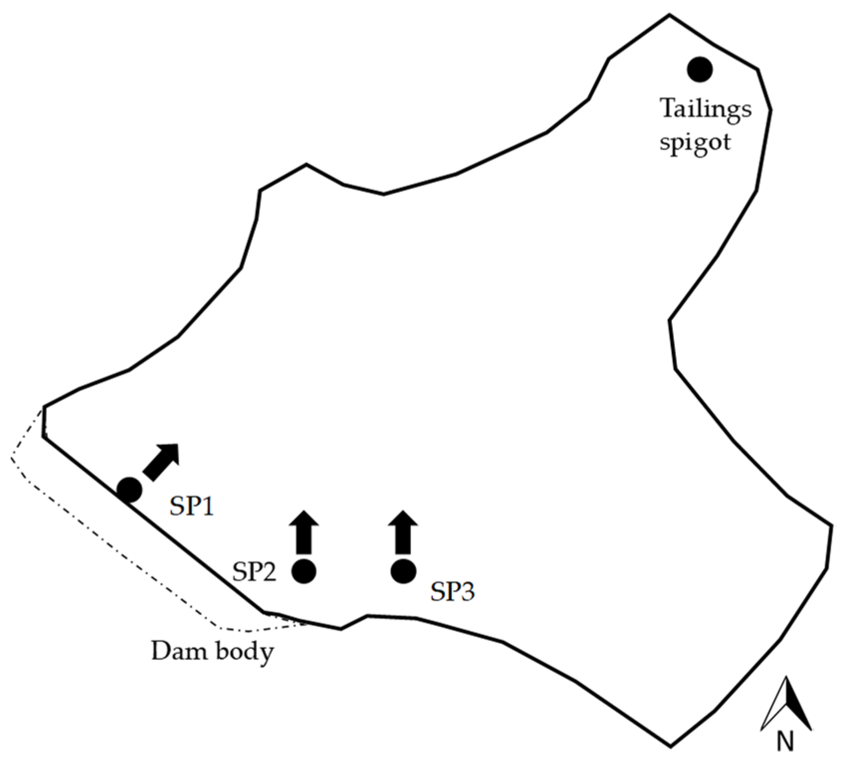
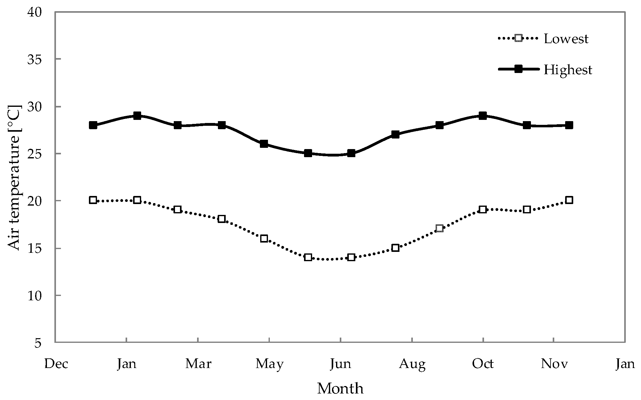
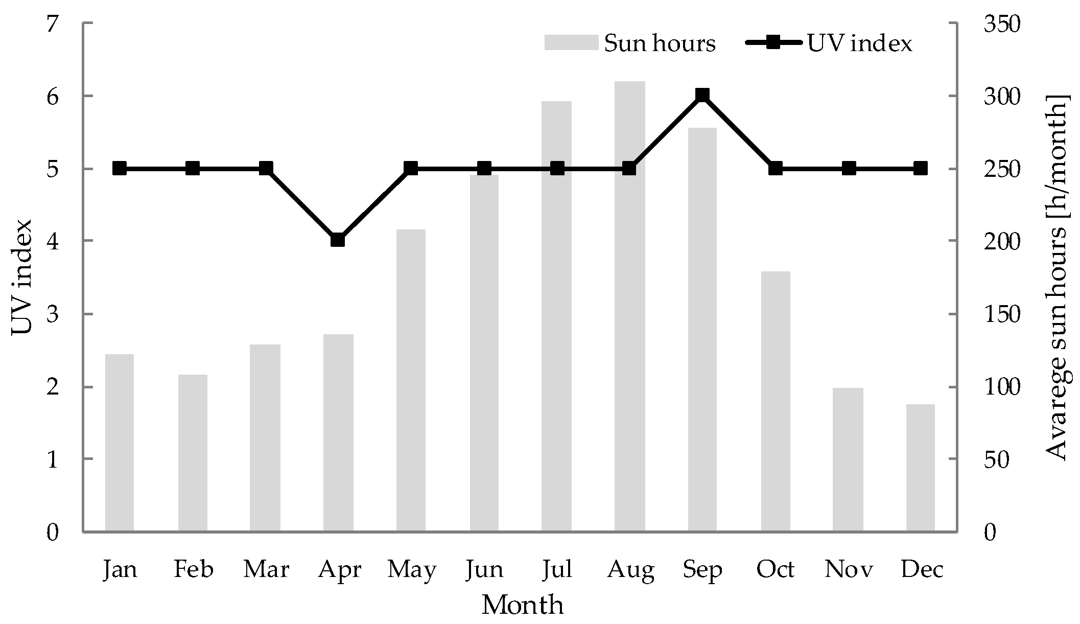
3.2. Field Exposure Conditions

The geomembrane was installed in Brazil in a location with a temperate climate, with an average annual temperature of around 23 °C and a rainfall rate of approximately 1400 mm/year. The average altitude is 650 m above sea level. In this region, summer (December–March) is marked by high temperatures and precipitation. Winter (June–September) is marked by lower temperatures, as well as lower amounts of precipitation. The highest UV index values are observed in spring (September–December), and the lowest values are seen in autumn (March–June). Despite these variations, the UV index value appears to remain stable throughout the months of the year, averaging around 5. Figure 2, Figure 3 and Figure 4 show graphs characterizing the climate of the exposure site, representing the variation in the average values of the lowest and highest temperatures measured by the local meteorological station in each month; the precipitation; the UV index; and sun h/month over a 1-year period.
In addition to being exposed to weathering from climatic conditions, samples 2 and 3 of the geomembrane were alternately exposed to chemical weathering caused by contact with the tailings from gold mining deposited in the reservoir.
Following extraction from the original mine, the run of mine (ROM) material is conveyed to the beneficiation plant, where the gold recovery process is initiated. This process comprises several key stages, including crushing, separation, gravity concentration, cyanide leaching, gold recovery, and the production of tailings. Additionally, the facility employs an industrial effluent treatment system to facilitate water reuse. The leaching process employs cyanide to enhance gold recovery, leading to the storage of cyanide tailings in a line dam due to their hazardous classification.
The tailings contained in the dam have levels of arsenic, iron, and sulfate significantly above the maximum permissible limits [69], indicating high potential for contamination. The cyanide value is slightly above the limit. The pH value indicates a slightly alkaline solution. Table 1 displays the levels of these constituents in the mining tailings compared to the maximum values from the standard [69].

4. Tests Methods

It is important to note that the tests were conducted outside the critical stress cracking zone (CRIT) and the squeeze-out and heat-affected zone (HAZ) on SP2. In other words, they were performed on the geomembrane sheet without seam influence, except for the specific seam tests (Section 4.8). All tests were conducted in accordance with the specific standards indicated below. Control variables were set, and uncertainties were minimized.

4.1. Density

These tests were conducted using an analytical balance with precision of 0.1 mg, following the procedures outlined in ASTM D792 [70], Method B. Five geomembrane specimens (for each sample), with a volume no less than 1 cm3, were weighed in air and in an immersion liquid, in this case alcohol (with a density of approximately 0.78 g/cm3), at 23 ± 0.5 °C. First, a specimen was weighed in air, and the mass was recorded. Subsequently, the specimen was fully immersed, ensuring any bubbles adhering to it were removed by gently rubbing the specimen with a wire. The apparent mass was then recorded immediately after immersion. The mass of the sample holder was also recorded. This procedure was repeated for each specimen. The specimens’ densities were calculated based on the calculation procedures presented in the standard and recorded.

4.2. Thickness

These tests were conducted using a gauge with a base and a free-moving foot plate, whose planar faces were parallel to each other within 0.01 mm, following the procedures outlined in ASTM D5199 [71]. The gauge had a 6.35 mm diameter presser foot and base. Force was applied to the presser foot on the base, and the initial base reading was recorded. Subsequently, the presser foot was raised, the specimen was centered on the base, and the pressure was gradually increased to 20 ± 0.2 kPa over a period of 5 s. Moisture equilibrium in the atmosphere was maintained throughout the execution, with a temperature of 21 ± 2 °C and relative humidity of 60 ± 10%. Ten specimens were evaluated for each sample. The average nominal thickness was reported.

4.3. Tensile Tests

These tests were conducted using an EMIC DL3000 machine (EMIC, Tokyo, Japan), following the procedures outlined in ASTM D6693/D6693M [72]. The tests were conducted in a standard laboratory atmosphere of 21 ± 2 °C. Ten dumbbell-shaped specimens (Type IV) were used for each sample, and tests were performed in both the machine and transverse directions. The testing speed was set at 50 mm/min until specimen brake. The specimen was securely placed in the grips, ensuring even and firm tightening to prevent slippage during the test. The load–extension curve of the specimen was then recorded. The results obtained included the yield and break strengths and strains.

4.4. Tear Resistance

These tests were conducted using an EMIC DL3000 machine following the procedures outlined in ASTM D1004 [73]. Ten specimens (for each sample) were cut in both the machine and transverse directions. Standardized atmospheric conditions were maintained throughout the execution, with a temperature of 23 ± 2 °C and relative humidity of 50 ± 10%. A jaw separation of 25.4 mm was employed, and the testing speed was set at 51 mm/min. The maximum load and maximum extension were measured, and the results served as an index for evaluating the geomembrane’s ability to resist tear propagation.

4.5. Puncture Resistance

These tests were conducted using an EMIC DL3000 machine following the procedures outlined in ASTM D4833/D4833M [74]. The minimum specimen diameter was 100 mm, and they were clamped between plates featuring a 45 ± 0.025 mm circular aperture. Five specimens were examined for each sample. An 8 ± 0.1 mm puncture probe with a flat end with a 45° = 0.8 mm chamfered edge was employed. The specimen was centered and secured between the holding plates, ensuring it extended beyond the outer edges of the clamping plates. The testing speed was set at 300 ± 10 mm/min until specimen rupture. The maximum load and the corresponding deformation were measured, and the results served as an index for evaluating the geomembrane’s capability to withstand concentrated loads.

4.6. Carbon Black

To evaluate the carbon black content in the geomembrane, a test was conducted using a muffle furnace with dimensions of approximately 100 mm by 100 mm by 100 mm, following the procedures outlined in ASTM D4218 [75]. Three specimens were cut from each exhumated sample. The muffle furnace was placed in a fume hood, and the controller indicator was set to 600 °C and stabilized at 610 °C. An aluminum dish was weighed and placed in the muffle furnace to burn off the surface oil for 2 min. The dish was then transferred to a desiccator and allowed to cool for 2 min. The weight of the dish was recorded. Then, 1 g of the specimen was added, and the dish was reweighed. The dish was placed back in the muffle furnace for 3 min until no ashable fillers remained. After this, the dish was placed in the desiccator to cool for 2 min. After material combustion, the residue was collected and weighed to estimate the percentage of carbon black present in the material. This test allowed for the assessment of the geomembrane’s composition.
The test to evaluate the dispersion of carbon black in the geomembrane was conducted according to the standard ASTM D5596 [76]. Ten specimens were examined for each sample. A microtome with a sample clamp and a knife holder was used to prepare microsections of the geomembrane samples (each approximately 2.54 cm) in the cross-machine direction. Each thin section was approximately 10 μm thick. Microscopic evaluation was performed using equipment that allowed us to view it at 100× magnification. Five specimens were mounted onto each slide and placed under the microscope. The microscope was set up for transmitted light microscopy, with the calibrated reticle positioned between the eyepiece lens and the objective. The microscopic analysis was conducted to locate the largest carbon agglomerate or inclusion, and its area was calculated. All the readings and calculations were recorded, and the results were rounded to the nearest whole number. The visualizations were classified according to the table provided in the Adjunct to ASTM D5596 [76].

4.7. Stress Crack Resistance (SCR)

The test conducted was the single point-notched constant tensile load test (SP-NCTL), following the procedures established by ASTM D5397 [77]. Five test specimens (for each sample) were immersed in a solution with reagent consisting of 10% Igepal CO-630 and 90% deionized water. The thickness of each individual test specimen was measured. In each specimen, a notch was made with a constant ligament thickness equal to 80% ± 1% of the nominal thickness of the geomembrane. The specimens were then loaded at various percentages of their yield stress, with the stress levels applied ranging from 20% to 65% in maximum increments of 5%. The yield stress of the material was measured. The test bath was filled with reagent, and the temperature was adjusted to 50 ± 1 °C. The test specimens were attached to hooks, and the distance between the lever arm and the switch was set to 20 mm. The specimens were then immersed, and the temperature was allowed to reach equilibrium for at least 30 min. Each specimen was loaded with its respective weight, and the elapsed time to failure was recorded. The obtained value from the calculations presented by the standard was related to the material’s resistance to crack initiation and propagation under tensile stress and in the presence of chemical agents that might accelerate the failure process.

4.8. Integrity of the Seams

Peel and shear tests were conducted following the procedures established by ASTM D6392 [78]. Grip faces 25 mm wide and with a 25 mm length were used. For both tests, a die measuring 25 mm in width and 150 mm in length was employed to cut the specimens. A standardized laboratory environment was maintained throughout the executions, with a temperature of 21 ± 2 °C and relative humidity between 50 and 70%. A constant machine crosshead was set at 50 mm/min. For the peel test, five specimens were each fully gripped across its width and subjected to the 90° T-peel test until failure, whereas for the shear test, the testing concluded when the specimens had elongated by 50%. The obtained values were used to evaluate whether the welded seams met the performance and durability standards.

4.9. Oxidative Induction Time (OIT) Tests

Std-OIT (standard oxidative induction time) and HP-OIT (high-pressure oxidative induction time) tests were performed on two specimens for each excavated sample using a differential scanning calorimeter (DSC, TA Instruments Q20 series). The Std-OIT test was conducted at 200 °C [79], while the HP-OIT test was conducted at 150 °C and 3.4 MPa [80], in accordance with their respective standards. In both tests, the specimens were heated at a constant rate, and once the specified temperature was reached, the material was held at this constant temperature until the oxidative reaction appeared on the thermal curve. Both tests were conducted to assess the availability of antioxidants in the exhumated geomembrane samples. The OIT tests were conducted in 2020. Therefore, the Std-OIT test was conducted following ASTM D3895 [79] instead of the ASTM D8117 recommendations [81], as the alteration in the GRI GM13 standard [45] indication regarding which standard to follow was made in March 2021.
After conducting the tests, the results were analyzed using the concept that the degradation of a geomembrane consists of three stages depending on the level of antioxidants (oxidative induction time (OIT) performance). Nominal failure was defined as a reduction in a selected physical property (in this case, stress crack resistance (SCR) and tensile strength were analyzed) to 50% of the minimum value specified by the GRI GM13 standard [45]. Non-parametric statistics were applied to analyze the probability of success of the geomembrane as a hydraulic barrier in the reservoir.

5. Test Results

Table 2 shows the average values and coefficients of variation (CVs) obtained for each geomembrane test. Since the authors did not have access to the initial geomembrane data prior to exposure, the analysis was based on the values established by the GRI GM13 standard [45] at the time of the geomembrane’s installation. This standard is a specification developed by the Geosynthetic Institute (GRI) for the test methods, test properties, and testing frequency for smooth and textured high-density polyethylene (HDPE) geomembranes. It sets minimum values for the physical, mechanical, and chemical properties that the geomembrane must meet or exceed [45].
For all the samples, the average values for tear resistance, puncture resistance, and carbon black content were higher than those recommended by GRI GM13 [45]. The CVs for the density, thickness, tensile strength, and strain are sufficient to account for any difference between the average values from the results and those recommended by that standard. The intrinsic variability of the geomembrane, even within the same batch (SP2 and SP3), contributes to such variations represented by the CVs. All the specimens from all the samples were categorized as Category 1, according to ASTM D5596 [76]. However, for SCR (with the exception of SP1), Std-OIT, and HP-OIT, the CVs do not account for the difference between the average values of the results and those recommended by the GRI GM13 standard [45]. It is important to note that the geomembrane was installed in 2009 (SP2 and SP3) and 2013 (SP1—raising). At these times, the minimum recommended SCR value according to the standard was 300 h, and there are no records of changes in the tensile strain or OIT values.
High values for the CVs (greater than 20%) were observed for tensile strength and strain at break. These elevated values are attributable to an outlier in the dataset. Excluding this outlier would reduce the respective coefficients of variation from 27.3% to 16.3% and from 20.8% to 13.7%. While still significant, such magnitudes are justifiable, as samples exposed to weathering typically exhibit greater variability in durability test results [44,46].
Table 3 shows the average values and coefficients of variation (CVs) obtained in the shear and peel tests for the seam specimens. Since the authors did not have access to the initial data prior to exposure, the analysis was based on the values established by GRI GM19a [82]. GRI GM19a [82] is a standard specification developed by the GRI for the seam strength and related properties of thermally bonded homogeneous polyolefin geomembranes. It establishes the required seam strength and properties for thermally bonded, non-reinforced polyolefin geomembranes, including HDPE, LLDPE, and flexible polypropylene (fPP).
As outlined in [82], the mode of rupture AD-BRK with more than 25% separation is considered unacceptable for HDPE geomembranes. Furthermore, according to this standard, the peel separation should not exceed the given values, and in this case, the CVs do not account for the difference between the average values from the results and those recommended by [82].
High values for the CVs (in this case, greater than 40%) were identified for the shear elongation at break and the peel separation in weld A. Since this analysis was conducted on only five specimens, as per the standard [78], the presence of an outlier significantly influenced these values. By excluding the outlier, the coefficients of variation would have decreased to 20.6% and 21.2%, respectively. These values remain high but are acceptable considering the variability of the data after weather exposure and the inherent variability in the geomembrane welding processes in the field [44,46].

6. Discussion

The aging of HDPE geomembranes might eventually lead to degradation and reductions in their mechanical properties by more than 50% from the values established by the GRI GM13 standard [45], ultimately resulting in material nominal failure [30,34,35,36,37,38,39,40,41,42,43,44]. The results obtained from the Std-OIT and HP-OIT tests (Table 2) for the case study in question show that all the samples fall below the minimum values required for satisfactory performance according to the [45] standard, showing evidence of the depletion of antioxidants due to exposure to the boundary conditions. The Std-OIT and HP-OIT values measured for the different samples exhumed from the dam reservoir (SP1, SP2, and SP3) were statistically different (Figure 5). SP1 showed higher values in all the oxidation tests compared to SP2 and SP3, as expected, given that its exposure time was 4 years less. Between SP2 and SP3, which came from the same batch and were exposed to climatic and chemical weathering (tailings) for the same duration, the results for SP3 were slightly lower than those for SP2.
Both samples, SP2 and SP3, were taken from similar heights and nearby regions on the upstream slope of the dam, with variations in the elevation of the tailings within the reservoir during the exposure time. Considering the solar dynamics in the southern hemisphere (where the tailing dam is located), the steeper slope (SP3 at 0.67°) received slightly more direct sunlight. In this context, the steeper slope allowed SP3 to receive a slightly more perpendicular incidence of sunlight, enhancing the total solar irradiation received. This slightly increased its exposure to ultraviolet light (UV), and consequently, the longer duration for which the geomembrane was subjected to elevated temperatures may have contributed to the slightly difference in the OIT values between the samples since UV radiation is capable of generating free radicals by attaching polymer chains [29,31,35,44,46].
A variable that could also be highlighted as a possible contributor to this slight difference would be the distribution of carbon black in the amorphous zones of the material, which can influence how the polymer chains interact and, consequently, the mechanical properties, as poor distribution could result in weak points in the geomembrane. However, it is important to note that the carbon black dispersion test was conducted in accordance with ASTM D5596 [76], and both samples were classified as Category 1. A more probable contributing factor to this slight difference in values between the samples is the inherent variability of the geomembrane stemming from its manufacturing process.
According to the theory that the degradation of a geomembrane consists of three stages [29,30,31,32,33,34] (Figure 6), the average residual values of Std-OIT and HP-OIT for HDPE geomembranes are presented in the literature as around 2 min and 70–100 min, respectively [30,31,35,83]. These values can vary depending on the geomembrane, resin type, exposure conditions, and synergistic or antagonistic effects of the degradation mechanisms [29,31]. Considering this, geomembrane SP2 and especially geomembrane SP3 could be very close to, or have already reached, their residual stages (the end of the first stage) for Std-OIT and HP-OIT, while SP1 is likely in the first stage.
The results of the tensile tests, both at yield and break points, show that all the samples had average values that were satisfactory, considering the coefficient of variation (CV), when compared to the minimum values established by the GRI GM13 standard [45], and there is no statistically significant difference between them (Figure 7). This could suggest that despite the consumption of antioxidants and stabilizers in the geomembrane, no significant signs of physical degradation were observed in terms of a significant decrease in tensile strength properties. This would likely indicate that the material was still in the first (SP1) and second (SP2 and SP3) stages of the three-stage degradation model of geomembranes.
However, when evaluating the results on the SCR, samples SP2 and SP3, which were exposed to climatic and chemical weathering conditions (tailings) for 11 years, had average values that were less than 50% of those established by the GRI GM13 standard [45] (Figure 8), which means that they reached nominal failure. Ref. [31], when analyzing HDPE geomembranes with different types of resin and under varying exposure conditions, suggests that a change in the SCR due to morphological changes may be an important factor contributing to its reduction in value. Other factors that may also contribute to the reduction in the SCR, according to the prior authors, include surface scratches, caused by installation damage, and/or surface oxidation.
The SP-NCTL test was not conducted on either surface of the geomembrane (exposed or in contact with the dam), so it was not possible to determine whether the surface in contact with the soil had lower SCR values compared to the exposed surface. Therefore, it was not possible to rule out the possibility that surface scratches and/or surface oxidation contributed to the low SCR values.
Ref. [31] observed a reduction in the SCR values before antioxidant depletion and before it was possible to observe evidence of geomembrane chemical degradation. The author related this fact to morphological changes during the aging process that were capable of affecting the inter-lamellar connections due to chain disentanglement. In chain disentanglement, the inter-lamellar connections of the crystalline lamellae decrease, and the material can become more prone to cracking. Ref. [34] states that the extent of these morphological changes will vary depending on the exposure conditions of the geomembrane, as well as the thermal and stress history experienced during the manufacturing process, which affects the orientation of the crystal lamellae. Therefore, the possibility that the reduction in the SCR was due to chain disentanglement cannot be ruled out. It is not possible to determine the main factor responsible for the decrease in the SCR values.
It is important to note that even though the geomembrane may have reached its nominal failure based on the SCR values, this does not imply that actual failure of the geomembrane in the field application is imminent. Despite these low values, the geomembrane had not yet ruptured based on visual inspection. This behavior is consistent with findings presented in the literature, such as [31], who also evaluated an HDPE geomembrane exposed in a mining facility in a warm–hot climate. Their study reported the HDPE geomembrane reaching nominal failure based on the SCR, with the geomembrane showing no signs of actual rupture in the field, despite extremely low SCR values being observed at certain analysis points.
Although the points mentioned above are considered and the three-stage degradation model taken into account (Figure 6), the geomembrane still appears to be in the second stage of degradation (antioxidant-depleted), as there was no evidence of chemical degradation in terms of changes in its tensile strength properties.
Considering this, non-parametric statistics were applied, utilizing the KDE to obtain a probability density function (PDF) that best represented the behavior of the geomembrane as a function of tensile strength under the given boundary conditions (Figure 9). With the application of non-parametric statistics, for each data point, a function was created centered on those data, and the PDF was estimated according to the sum of these cores divided by the total number of specimens [84,85]. Thus, it was not necessary to check the fit of the data to a previously known distribution.
Parametric statistical methods are quite widespread in the literature, but these methods come with a caveat: the requirements of a set of assumptions about the data’s underlying distribution. In other words, this means that knowledge of the PDF for the data under study is a prerequisite. However, proposing an incorrect PDF can introduce estimation errors and compromise the reliability of the statistical conclusions. In contrast, non-parametric statistical methods offer a more flexible alternative, free from the constraints of distributional assumptions. Among these, methods based on the KDE have gained prominence [86]. In practice, the KDE provides a straightforward way to structure datasets without imposing a specific parametric model, making it a valuable tool in data analysis [87].
In situations where the sample data present marked asymmetry effects or the presence of outlier values, among other unusual situations, using strategies independent of the previous proposition of a PDF becomes a powerful option. Using the PDF obtained via the KDE is a straightforward approach that results in a smoother and more continuous representation of the proper distribution of the sample data. These PDFs (Figure 9), shaped by the KDE, can reflect local patterns in the data and capture nuances and details that may be missed using more rigid methods. Simultaneously, the KDE helped smooth out noise present in the data and provided more precise insights into the overall behavior.
It is evident that for this specific exposure scenario and this particular geomembrane, the PDF does not fit any known parametric statistical distribution. A new sampling experiment might yield distinct PDFs. From a purely theoretical standpoint, to thoroughly analyze the behavior of these PDFs, it would be necessary to repeat the experiment multiple times in multiple scenarios and examine whether any consistent patterns emerge. This approach allows for a comprehensive understanding of the variability and characteristics of the PDFs. Given the multimodal nature of these PDFs, identifying any discernible patterns is particularly challenging, as the complexity and variability make it difficult to visualize a consistent trend. Altering the exposure conditions, time, and/or the geomembranes will result in different PDFs, which means that it is not possible to generalize the PDFs shown in Figure 9.
These PDFs enabled the determination of the probability of nominal failure of the geomembrane (when the tensile strength is reduced to 50% of the minimum value specified by the GRI GM13 standard [30,34,35,36,37,38,39,40,41,42,43,44,45]) under the given time and exposure conditions as a function of tensile strength. The geomembrane’s probability of nominal failure for the specific exposure time and the conditions of SP1, SP2, and SP3 was 0%, 0%, and 0.4%, respectively. These probability values were calculated by integrating the area under the PDF for tensile strength values less than 26.5 kN/m; according to the densities of SP1 and SP2, the probability was zero, whereas with the density of SP3, the probability was non-zero. This can be observed according to the shaded area under the PDF curve in Figure 9c. This means that assuming SP1, SP2, and SP3 together are representative of the geomembrane covering the reservoir of the dam, even with conservative estimation, the probability of the geomembrane reaching nominal failure is 0.4% as a function of tensile strength.
It is important to note that the studied samples were either above the tailings or at elevations influenced by the variation in the tailing elevation. Therefore, this assessment of geomembrane durability cannot be directly applied to sections of it that are completely submerged in the dam reservoir.
Regarding the representativeness of the samples and considering their tensile strength (for which the non-parametric statistical analysis was conducted), it is substantially adequate considering the literature data for similar situations [44,46]. Variations and uncertainties are inherent to the samples, especially after an exposure period. Therefore, it would be necessary to replicate the experiments to identify distribution patterns and consequently analyze behavioral representativeness. This approach would lead to a better understanding of the variables involved and contribute to the robustness of the obtained results.
Another point of analysis is the performance of the seam. Although the peel strength exhibited satisfactory values when compared to the minimum requirement established by the [82] standard, the peel separation showed values higher than the maximum allowable values, even when considering its variability (Figure 10). According to [62], unsatisfactory peel separation does not necessarily imply loss of the bonded area, but it does not exclude this possibility. Depending on the geomembrane/seam combination, it could induce crazing, which serves as a precursor to stress cracks.
Even though the SCR tests were conducted outside the CRIT zone, comparing samples SP2 and SP3 (Figure 8), which were installed with geomembranes from the same batch and under similar exposure conditions, shows no statistically significant difference in the SCR values. This likely contributes to the understanding that even if crazing has been induced in the CRIT zone, it has not influenced the behavior of the geomembrane sheet in terms of SCR performance.
Additionally, ref. [62] also mentions that the separation of a seam during testing may indicate that at some point during the geomembrane’s service life, this seam could come apart if it is located over a subsided subgrade, on a fold, or even at waves caused by thermal expansion/contraction. If the seam comes apart, the geomembrane will no longer be able to serve its function as a hydraulic barrier in the reservoir of the dam.
It is noteworthy that the company conducting the mining operations in question, aiming to comply with the requirements of the Brazilian National Mining Agency (ANM), conducted environmental analyses to assess whether there were any signs of significant contamination in the area, as the SCR and peel separation test values were unsatisfactory. These analyses indicated no significant indications; however, the authors were not granted permission to publish them.
When considering the possibility of catastrophic consequences due the geomembrane failure within the context of mining operations, analyzing the probability of failure becomes essential for decision-making regarding preventive or corrective actions. Despite reaching nominal failure for the SCR and exhibiting unsatisfactory performance in the peel separation tests, the geomembrane continues to fulfill its primary function as a hydraulic barrier. With a minimal probability of reaching nominal failure in terms of tensile strength at 0.4%, this translates to a 99.6% probability of successfully preventing the percolation of contaminants from the tailings reservoir. This not only ensures the integrity of the groundwater resources but also enhances the safety of drinking water sources downstream. Moreover, by containing pollutants within the reservoir, the geomembrane plays a pivotal role in mitigating their impact on local flora and fauna.
The adequate performance of the geomembrane, specifically within the context of mining tailings reservoirs, aligns with the Sustainable Development Goals (SDGs). Although the SDGs are interdependent, the success of the geosynthetic barrier directly supports goals such as Goal 6 (Clean Water and Sanitation) and Goal 15 (Life on Land), as well as Goal 3 (Good Health and Well-being), Goal 9 (Industry, Innovation, and Infrastructure), Goal 11 (Sustainable Cities and Communities), Goal 12 (Responsible Consumption and Production), and Goal 13 (Climate Action), while also contributing to other SDGs in a transversal manner [15]. Thus, this application of geomembranes underscores their critical contribution to sustainable mining practices and global environmental conservation efforts.
Furthermore, by employing non-parametric statistical methods, we provide a viable approach to assessing the probability of success of geomembranes as hydraulic barriers, despite the numerous variabilities among the application scenarios of HDPE geomembranes in mining tailings reservoirs. The findings underscore the importance of considering the unique environmental and operational conditions of each installation when evaluating geomembrane performance. Also, they contribute to a broader understanding of geomembrane durability and reliability, offering valuable guidance for future applications in similar contexts.

7. Conclusions

This study investigated the degradation that occurred in the properties of an exposed HDPE geomembrane installed at a gold mining tailing site in Brazil in a warm–hot climate. Non-parametric statistics were applied to help with the analysis. For the specific geomembranes and conditions examined, the following was concluded:
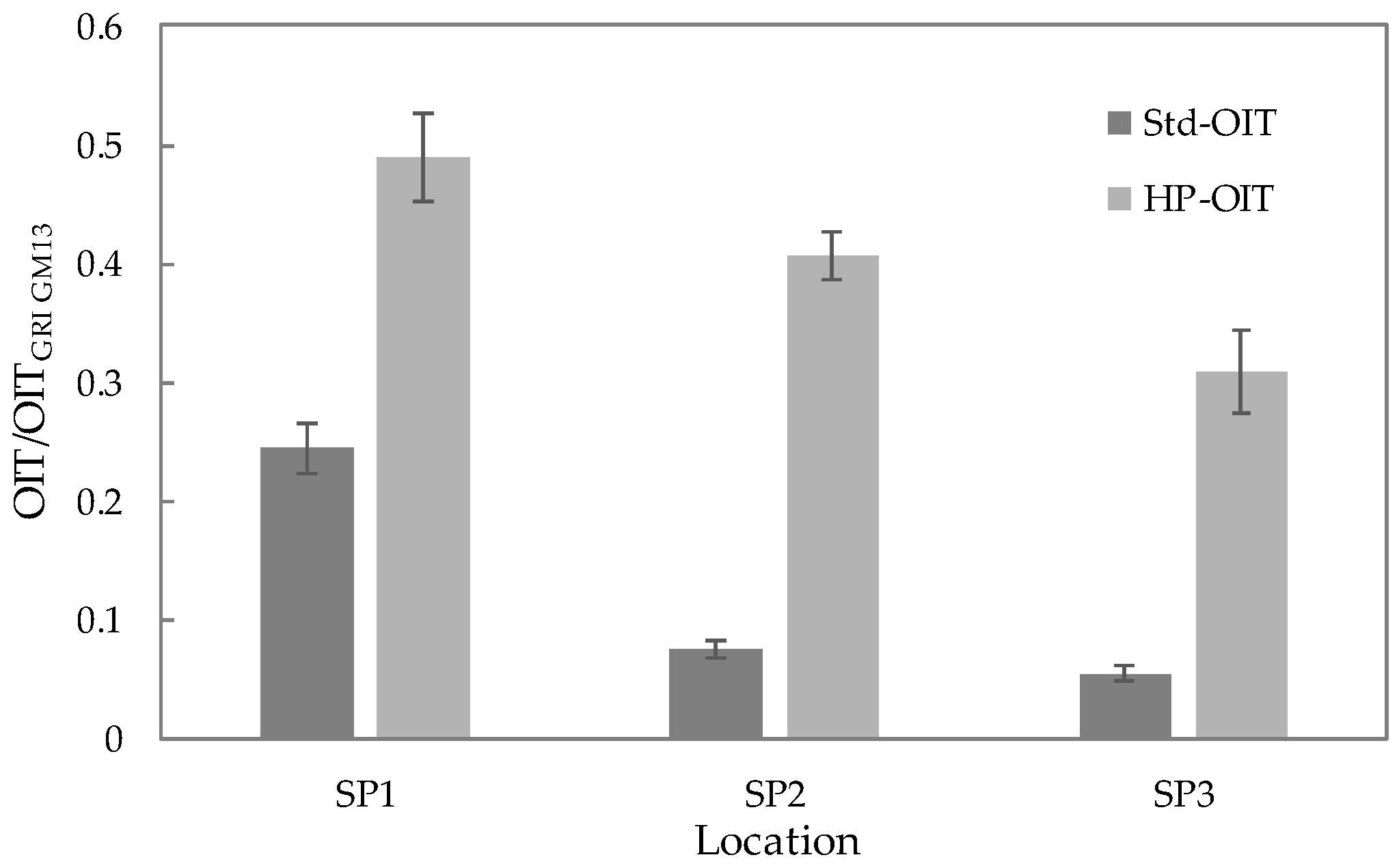
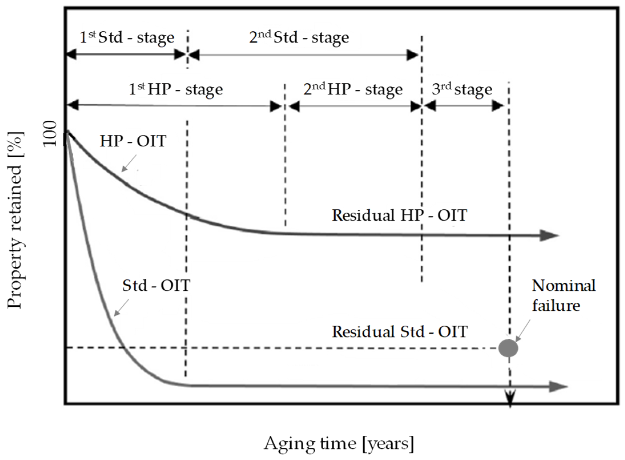
  • The geomembrane exposed showed antioxidant depletion, but considering the average residual values of Std-OIT and HP-OIT for HDPE geomembranes from the literature [30,31,35,83], it is possible that there are still antioxidant stabilizers to be consumed (first stage of degradation) for SP1. SP2 and especially SP3 could be very close to, or have already reached, their residual values.
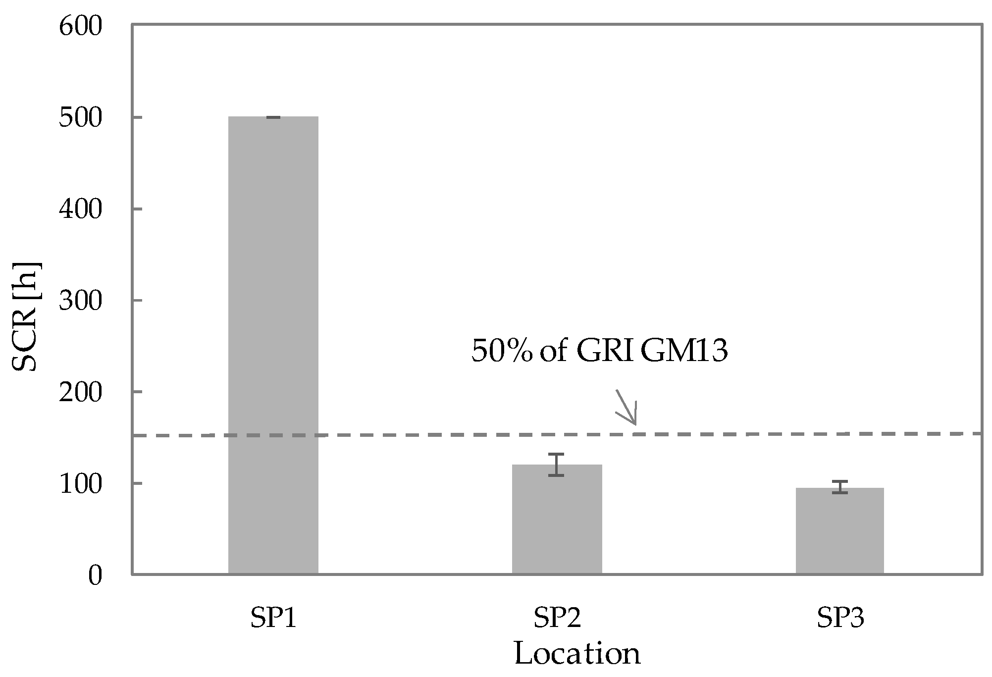
  • After 11 years of exposure, the SCR values of SP2 and SP3 had decreased to 40 and 32% of the reference value [45], implying that the material had reached nominal failure.
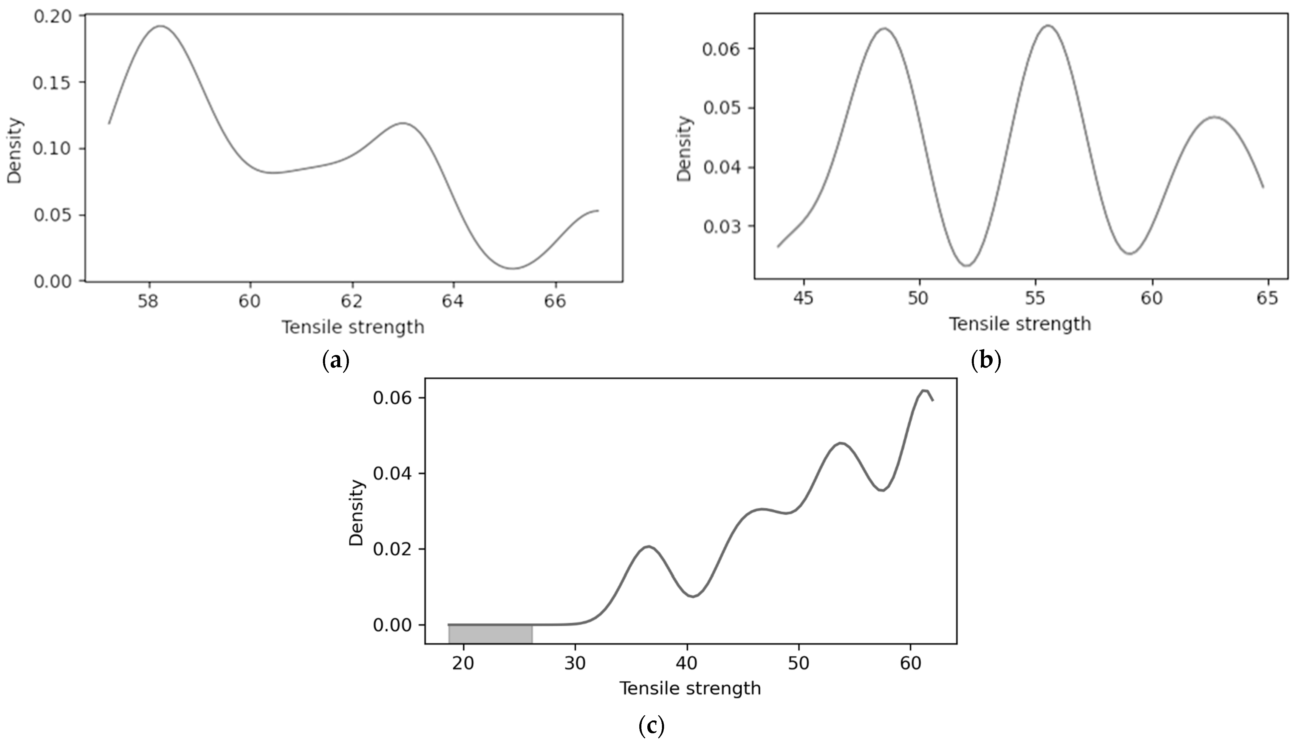
  • The probability of the geomembrane reaching nominal failure was 0.4% as a function of tensile strength, which translates to a 99.6% probability of success.
  • The peel separation showed values higher than the maximum values allowable [45]. Environmental analyses indicated no significant contamination in the area.
  • The geomembrane used in this scenario contributed to SDG 3 (Good Health and Well-Being), SDG 6 (Clean Water and Sanitation), SDG 15 (Life on Land), and SDG 13 (Climate Action).
Chemical weathering from seasonal tailings contact (samples SP2 and SP3) and climatic weathering did not significantly degrade the geomembrane compared to sample SP1, which faced only climatic weathering. Varying exposure times prevent definitive conclusions. While the geomembrane’s nominal failure may be indicated by the SCR values, this does not imply imminent failure in the field but warns of substantial reductions in its properties and its potential susceptibility to failure based on its remaining resistance and the site conditions.
Future research should focus on verifying consistent patterns in the probability density functions (PDFs) by exploring a variety of exposure conditions, durations, and geomembrane types. Such studies are essential to better understand the long-term performance and degradation mechanisms of geomembranes under diverse environmental and operational scenarios. Additionally, investigations into different installation practices and their impact on geomembrane durability will provide valuable insights. By broadening the scope of research to include these variables, it is possible to develop more robust predictive models and enhance the reliability and sustainability of geomembrane applications in mining and other industries. The results obtained using Kernel Density Estimators were promising for evaluating the exhumed geomembrane samples. This methodology may be extended to other engineering projects involving various types of geosynthetics, whether exhumed or aged in a laboratory, thereby enhancing their reliability.

Author Contributions

Conceptualization, B.M.C.U.; data curation, B.M.C.U. and R.S.; formal analysis, B.M.C.U. and R.S.; investigation, R.S.; methodology, B.M.C.U. and A.R.D.; supervision, L.D.F., T.I. and D.C.U.; validation, L.D.F., T.I. and D.C.U.; writing—original draft, B.M.C.U.; writing—review and editing, B.M.C.U., R.S., L.D.F., T.I., D.C.U. and A.R.D. All authors have read and agreed to the published version of the manuscript.

Funding

A.R.D. received additional support from Federal University of Ouro Preto.

Institutional Review Board Statement

Not applicable.

Informed Consent Statement

Not applicable.

Data Availability Statement

The data that support the findings of this study are available from the corresponding author [Beatriz M. C. Urashima] upon reasonable request.

Acknowledgments

We are grateful to Federal University of Ouro Preto, Osaka University, Japan International Cooperation Agency and Federal Center for Technological Education of Minas Gerais for the support.

Conflicts of Interest

The authors declare no conflicts of interest.

References

  1. Pinto, G.E.; Pires, A.; Georges, M.R.R. Anthropocene and climate change: The perception and awareness of Brazilians according to the IBOPE survey. Desenvolv. Meio Ambiente 2020, 54, 1–25. [Google Scholar] [CrossRef]
  2. Thomas, L.; Tang, H.; Kalyon, D.M.; Aktas, S.; Arthur, J.D.; Blotevogel, J.; Carey, J.W.; Filshill, A.; Fu, P.; Hsuan, G.; et al. Toward better hydraulic fracturing fluids and their application in energy production: A review of sustainable technologies and reduction of potential environmental impacts. J. Pet. Sci. Eng. 2019, 173, 793–803. [Google Scholar] [CrossRef]
  3. Zhu, Y.; Zhang, F.; Jia, S. Embodied energy and carbon emissions analysis of geosynthetic reinforced soil structures. J. Clean. Prod. 2022, 370, 133510. [Google Scholar] [CrossRef]
  4. Palmeira, E.M.; Araújo, G.L.S.; Santos, E.C.G. Sustainable Solutions with Geosynthetics and Alternative Construction Materials—A Review. Sustainability 2021, 13, 12756. [Google Scholar] [CrossRef]
  5. Raja, J.; Dixon, N.; Fowmes, G.; Frost, M.; Assinder, P. Obtaining reliable embodied carbon values for geosynthetics. Geosynth. Int. 2015, 22, 393–401. [Google Scholar] [CrossRef]
  6. Slaymane, R.A.; Solimen, M.R. Integrated water balance and water quality management under future climate change and population growth: A case study of Upper Litani Basin, Lebanon. Clim. Chang. 2022, 172, 28. [Google Scholar] [CrossRef]
  7. Mousavi, S.H.; Kavianpour, M.R.; Alcaraz, J.L.G.; Yamini, O.A. System Dynamics Modeling for Effective Strategies in Water Pollution Control: Insights and Applications. Appl. Sci. 2023, 13, 9024. [Google Scholar] [CrossRef]
  8. Buber, A.; Bolgov, M.; Buber, V. Statistical and Water Management Assessment of the Impact of Climate Change in the Reservoir Basin of the Volga–Kama Cascade on the Environmental Safety of the Lower Volga Ecosystem. Appl. Sci. 2023, 13, 4768. [Google Scholar] [CrossRef]
  9. Schussel, Z.G.L. Sustainable urban development—A possible utopia? Desenvolv. Meio Ambiente 2004, 9, 57–67. [Google Scholar] [CrossRef]
  10. Leite, A.C.C.; Alves, E.E.C.; Picchi, L. The multilateral climate cooperation and the promotion of the energy transition agenda in Brazil. Desenvolv. Meio Ambiente 2020, 54, 379–403. [Google Scholar] [CrossRef]
  11. Dixon, N.; Fowmes, G.; Frost, M. Global challenges, geosynthetic solutions and counting carbon. Geosynth. Int. 2017, 24, 451–464. [Google Scholar] [CrossRef]
  12. Le Blanc, D. Towards Integration at Last? The Sustainable Development Goals as a Network of Targets. Sustain. Dev. 2015, 23, 176–187. [Google Scholar] [CrossRef]
  13. Cenci, D.R. Sociopolitical and Environmental Conflicts in the Brazilian Context: Before and After Rio 92, Environmental Policies and the Contribution to Latin American Geopolitics. Estud. Av. 2018, 30, 23–49. [Google Scholar]
  14. Lim, M.M.L.; Jorgensen, P.S.; Wyborn, C.A. Reframing the sustainable development goals to achieve sustainable development in the Anthropocene—A systems approach. Ecol. Soc. 2018, 23, 22. [Google Scholar] [CrossRef]
  15. Touze, N. Healing the world: A geosynthetics solution. Geosynth. Int. 2021, 28, 1–31. [Google Scholar] [CrossRef]
  16. Gutiérrez-Diez, J.C.; Castañón, A.M.; Bascompta, M. New Method to Study the Effectiveness of Mining Equipment: A Case Study of Surface Drilling Rigs. Appl. Sci. 2024, 14, 2185. [Google Scholar] [CrossRef]
  17. Tao, Y.; Zhang, R. An Integrated Decision Support System for Low-Disturbance Surface Mining. Appl. Sci. 2024, 14, 1672. [Google Scholar] [CrossRef]
  18. Trovão, J.; Soares, F.; Paiva, D.S.; Pratas, J.; Portugal, A. A Snapshot of the Microbiome of a Portuguese Abandoned Gold Mining Area. Appl. Sci. 2024, 14, 226. [Google Scholar] [CrossRef]
  19. Windisch, J.; Gradwohl, A.; Gilbert, B.M.; Dos Santos, Q.M.; Wallner, G.; Avenant-Oldewage, A.; Jirsa, F. Toxic Elements in Sediment and Water of the Crocodile River (West) System, South Africa, Following Acid Mine Drainage. Appl. Sci. 2022, 12, 10531. [Google Scholar] [CrossRef]
  20. Besedin, J.A.; Khudur, L.S.; Netherway, P.; Ball, A.S. Remediation Opportunities for Arsenic-Contaminated Gold Mine Waste. Appl. Sci. 2023, 13, 10208. [Google Scholar] [CrossRef]
  21. Ba, N.B.; Souissi, R.; Manai, F.; Taviche, I.K.; Bejaoui, B.; Bagga, M.A.; Souissi, F. Mineralurgical and Environmental Characterization of the Mine Tailings of the IOCG Mine of Guelb Moghrein, Akjoujt, Mauritania. Appl. Sci. 2024, 14, 1591. [Google Scholar] [CrossRef]
  22. American Society for Testing and Materials. Standard Terminology for Geosynthetics; American Society for Testing and Materials: West Conshohocken, PA, USA, 2024. [Google Scholar]
  23. Müller, W.W.; Saathoff, F. Geosynthetics in geoenvironmental engineering. Sci. Technol. Adv. Mater. 2015, 16, 034605. [Google Scholar] [CrossRef] [PubMed]
  24. Mounes, S.M.; Karim, M.R.; Khodaii, A.; Almasi, M.H. Improving Rutting Resistance of Pavement Structures Using Geosynthetics: An Overview. Sci. World J. 2014, 2014, 764218. [Google Scholar] [CrossRef]
  25. Markiewicz, A.; Koda, E.; Kawalec, J. Geosynthetics for Filtration and Stabilization: A Review. Polymers 2022, 14, 5492. [Google Scholar] [CrossRef]
  26. Brandl, H. Geosynthetics applications for the mitigation of natural disasters and for environmental protection. Geosynth. Int. 2011, 18, 340–390. [Google Scholar] [CrossRef]
  27. Zhang, Y.; Kinoshita, Y.; Kato, T.; Takai, A.; Katsumi, T. Attenuation performance of geosynthetic sorption sheets against arsenic subjected to compressive stresses. Geotext. Geomembr. 2023, 51, 179–190. [Google Scholar] [CrossRef]
  28. Giroud, J.P.; Bonaparte, R. Leakage through Liners Constructed with Geomembrane—Part I. Geomembrane Liners. Geotext. Geomembr. 1989, 8, 27–67. [Google Scholar] [CrossRef]
  29. Rowe, R.K.; Sangam, H.P. Durability of HDPE geomembranes. Geotext. Geomembr. 2002, 20, 77–95. [Google Scholar] [CrossRef]
  30. Ewais, A.M.R.; Rowe, R.K.; Scheirs, J. Degradation behaviour of HDPE geomembranes with high and low initial high-pressure oxidative induction time. Geotext. Geomembr. 2014, 42, 111–126. [Google Scholar] [CrossRef]
  31. Rowe, R.K.; Ewais, A.M.R. Ageing of exposed geomembranes at locations with different climatological conditions. Can. Geotech. J. 2014, 52, 326–343. [Google Scholar] [CrossRef]
  32. Hsuan, Y.G.; Koerner, R.M. Antioxidant depletion lifetime in high density polyethylene geomembranes. J. Geotech. Geoenviron. Eng. 1998, 124, 532–541. [Google Scholar] [CrossRef]
  33. Rowe, R.K.; Abdelaal, F.B.; Brachman, R.W.I. Antioxidant depletion of HDPE geomembrane with sand protection layer. Geosynth. Int. 2013, 20, 73–89. [Google Scholar] [CrossRef]
  34. Ewais, A.M.R.; Rowe, R.K.; Rimal, S.; Sangam, H.P. 17-year elevated temperature study of HDPE geomembrane longevity in air, water and leachate. Geosynth. Int. 2018, 25, 525–544. [Google Scholar] [CrossRef]
  35. Rowe, R.K.; Rimal, S.; Sangam, H. Ageing of HDPE geomembrane exposed to air, water and leachate at different temperatures. Geotext. Geomembr. 2009, 27, 137–151. [Google Scholar] [CrossRef]
  36. Hsuan, Y.G.; Schroeder, H.F.; Rowe, R.K.; Müller, W.; Greenwood, J.; Cazzuffi, D.; Koerner, R.M. Long-term performace and lifetime prediction of geosynthetics. In Proceedings of the EuroGeo4 Keynote Paper, Edinburgh, UK, 7–10 September 2008. [Google Scholar]
  37. Koerner, R.M.; Hsuan, Y.; Lord, A.E., Jr. Remaining technical barriers to obtaining general acceptance of geosynthetics. Geotext. Geomembr. 1993, 12, 1–52. [Google Scholar] [CrossRef]
  38. Müller, W.W.; Jakob, I.; Li, C.S.; Tatzky-Gerth, R. Durability of polyolefin geosynthetic drains. Geosynth. Int. 2009, 16, 28–42. [Google Scholar] [CrossRef]
  39. Scholz, P.; Putna-Nimane, I.; Barda, I.; Liepina-Leimane, I.; Strode, E.; Kileso, A.; Esiukova, E.; Chubarenko, B.; Purina, I.; Simon, F.-G. Environmental Impact of Geosynthetics in Coastal Protection. Materials 2021, 14, 634. [Google Scholar] [CrossRef] [PubMed]
  40. Sarsby, R.W. Geosynthetics in Civil Engineering; Woodhead Publishing Limited: Cambridge, UK, 2007. [Google Scholar]
  41. Koerner, R.M. Designing with Geosynthetics, 4th ed.; Prentice Hall: Upper Saddle River, NJ, USA, 2005. [Google Scholar]
  42. Koerner, R.M.; Hsuan, Y.G.; Koerner, G.R. Lifetime predictions of exposed geotextiles and geomembranes. Geosynth. Int. 2017, 24, 198–212. [Google Scholar] [CrossRef]
  43. Clinton, M.; Rowe, R.K. Long-term durability of two HDPE geomembranes formulated with polyethylene of raised temperature resistance (PE-RT). Geotext. Geomembr. 2024, 52, 304–318. [Google Scholar] [CrossRef]
  44. Rowe, R.K.; Shoaib, M. Effect of brine on long-term performance of four HDPE geomembranes. Geosynth. Int. 2017, 24, 508–523. [Google Scholar] [CrossRef]
  45. GRI GM13; Test Methods, Test Properties and Testing Frequency for High Density Polyethylene (HDPE) Smooth and Textured Geomembranes. Geosynthetic Research Institute: Folsom, PA, USA, 2024.
  46. Rowe, R.K.; Islam, M.Z.; Hsuan, Y.G. Leachate chemical composition effects on OIT depletion in an HDPE geomembrane. Geosynth. Int. 2008, 15, 136–151. [Google Scholar] [CrossRef]
  47. Lin, B.-H.; Yu, Y.; Bathurst, R.J.; Liu, C.-N. Deterministic and probabilistic prediction of facing deformations of geosynthetic-reinforced MSE walls using a response surface approach. Geotext. Geomembr. 2016, 44, 813–823. [Google Scholar] [CrossRef]
  48. Gilson-Beck, A. Controlling leakege through installed geomembranes using eletrical leak location. Geotext. Geomembr. 2019, 4, 697–710. [Google Scholar] [CrossRef]
  49. Akis, E.; Guven, G.; Loftfisadigh, B. Predictive models for mechanical properties of expanded polystyrene (EPS) geofoam using regression analysis and artificial neural networks. Neural Comput. Appl. 2022, 34, 10845–10884. [Google Scholar] [CrossRef]
  50. Agarwal, E.; Pain, A. Reliability assessment of reinforced slopes with unknown probability distribution. Geosynth. Int. 2023, 30, 337–349. [Google Scholar] [CrossRef]
  51. Chehade, H.Á.; Guo, X.; Dias, D.; Sadek, M.; Jenk, O.; Chehade, F.H. Reliability analysis for internal seismic stability of geosynthetic-reinforced soil walls. Geosynth. Int. 2023, 30, 296–314. [Google Scholar] [CrossRef]
  52. Ferreira, F.B.; Gomes, A.T.; Vieira, C.S.; Lopes, M.L. Reliability analysis of geosynthetic-reinforced steep slopes. Geosynth. Int. 2016, 23, 301–315. [Google Scholar] [CrossRef]
  53. Liu, H.; Zheng, J.; Zhang, R.; Xie, P. Probabilistic stability analysis of reinforced soil slope with non-circular RLEM. Geosynth. Int. 2023, 30, 432–448. [Google Scholar] [CrossRef]
  54. Abdelaal, F.B.; Rowe, R.K.; Morsy, M.S.; Silva, R.A. Deagradation of HDPE, LLDPE, and blended polyethylene geomembranes in extremely low and high pH mining solutions at 85 °C. Geotext. Geomembr. 2023, 51, 27–38. [Google Scholar] [CrossRef]
  55. International Geosynthetics Society. Guide to the Specification of Geosynthetics; International Geosynthetics Society: Jupiter, FL, USA, 2019. [Google Scholar]
  56. Heerten, G. Reduction of climate-damaging gases in geotechnical engineering practice using geosynthetics. Geotext. Geomembr. 2011, 30, 43–49. [Google Scholar] [CrossRef]
  57. Troost, G.H.; den Hoedt, G.; Risseeuw, P.; Voskamp, W.; Schmidt, H.M. Durability of a 13-Year Old Test Embankment Reinforced with Polyester Woven Fabric. In Proceedings of the Fifth International Conference on Geotextiles, Geomembranes and Related Products, Singapore, 5–9 September 1994. [Google Scholar]
  58. Buckley, J.; Gates, W.P.; Gibbs, D.T. Forensic examination of field GCL performance in landfill capping and mining containment applications. Geotext. Geomembr. 2012, 33, 7–14. [Google Scholar] [CrossRef]
  59. Leshchinsky, B.; Berg, R.; Liew, W.; Kawakami-Selin, M.; Moore, J.; Brown, S.; Kleutsch, B.; Glover-Cutter, K.; Wayne, M. Characterization of geogrid mechanical and chemical properties from a thirty-six year old mechanically-stabilized earth wall. Geotext. Geomembr. 2020, 48, 793–801. [Google Scholar] [CrossRef]
  60. Kiersnowska, A.; Fabianowski, W.; Koda, E. The Influence of the Accelerated Aging Conditions on the Properties of Polyolefin Geogrids Used for Landfill Slope Reinforcement. Polymers 2020, 12, 1874. [Google Scholar] [CrossRef]
  61. Rarison, R.F.M.; Mbonimpa, M.; Bussière, B.; Pouliot, S. Properties of HDPE Geomembrane Exhumed 20 Years After Installation in a Mine Reclamation Cover System. Int. J. Geosynth. Ground Eng. 2023, 9, 1. [Google Scholar] [CrossRef]
  62. Peggs, I.D. Destructive Testing of Polyethylene Geomembrane Seams: Various Methods to Evaluate Seam Strength. Geotext. Geomembr. 1990, 9, 405–414. [Google Scholar] [CrossRef]
  63. Gulec, S.B.; Benson, C.H.; Edil, T.B. Effect of Acidic Mine Drainage on the Mechanical and Hydraulic Properties of Three Geosynthetics. J. Geotech. Geoenviron. Eng. 2005, 131, 937–950. [Google Scholar] [CrossRef]
  64. Kaniki, A.T.; Tumba, K. Management of mineral processing tailings and metallurgical slags of the Congolese copperbelt: Environmental stakes and perspectives. J. Clean. Prod. 2018, 210, 1406–1413. [Google Scholar] [CrossRef]
  65. Clemente, J.S.; Huntsman, P. Potential climate change effects on the geochemical stability of waste and mobility of elements in receiving environments for Canadian metal mines south of 60 °N. Environ. Rev. 2019, 27, 478–518. [Google Scholar] [CrossRef]
  66. de Souza Neto, H.F.; da Silveira Pereira, W.V.; Dias, Y.N.; de Souza, E.S.; Teixeira, R.A.; de Lima, M.W.; Ramos, S.J.; do Amarante, C.B.; Fernandes, A.R. Environmental and human health risks of arsenic in gold mining areas in the eastern Amazon. Environ. Pollut. 2020, 265, 114969. [Google Scholar] [CrossRef]
  67. Doku, E.T.; Belford, E.J.D. Effect of heavy metals and physicochemical parameters on diversity of plants at a gold mine tailings dam in Ghana. J. Ecol. Nat. Environ. 2022, 14, 98–108. [Google Scholar] [CrossRef]
  68. Muñoz, J.M. Carbon foorprint of HDPE geomembrane vs. traditional waterproofing barrier. In Proceedings of the 12th International Conference on Geosynthetics, Rome, Italy, 17–21 September 2023. [Google Scholar]
  69. Brazilian Association of Technical Standards. Solid Waste—Classification; Brazilian Association of Technical Standards: Sao Paulo, Brazil, 2004. [Google Scholar]
  70. ASTM D792; Standard Test Methods for Density and Specific Gravity (Relative Density) of Plastics by Displacement. American Society for Testing and Materials: West Conshohocken, PA, USA, 2020.
  71. ASTM D5199; Standard Test Method for Measuring the Nominal Thickness of Geosynthetics. American Society for Testing and Materials: West Conshohocken, PA, USA, 2019.
  72. ASTM D6693/D6693M; Standard Test Method for Determining Tensile Properties of Nonreinforced Polyethylene and Nonreinforced Flexible Polypropylene Geomembranes. American Society for Testing and Materials: West Conshohocken, PA, USA, 2020.
  73. ASTM D1004; Standard Test Method for Tear Resistance (Graves Tear) of Plastic Film and Sheeting. American Society for Testing and Materials: West Conshohocken, PA, USA, 2021.
  74. ASTM D4833/D4833M; Standard Test Method for Index Puncture Resistance of Geomembranes and Related Products. American Society for Testing and Materials: West Conshohocken, PA, USA, 2020.
  75. ASTM D4218; Standard Test Method for Determination of Carbon Black Content in Polyethylene Compounds by the Muffle-Furnace Technique. American Society for Testing and Materials: West Conshohocken, PA, USA, 2020.
  76. ASTM D5596; Standard Test Method for Microscopic Evaluation of the Dispersion of Carbon Black in Polyolefin Geosynthetics. American Society for Testing and Materials: West Conshohocken, PA, USA, 2021.
  77. ASTM D5397; Standard Test Method for Evaluation of Stress Crack Resistance of Polyolefin Geomembranes Using Notched Constant Tensile Load Test. American Society for Testing and Materials: West Conshohocken, PA, USA, 2020.
  78. ASTM D6392; Standard Test Method for Determining the Integrity of Nonreinforced Geomembrane Seams Produced Using Thermo-Fusion Methods. American Society for Testing and Materials: West Conshohocken, PA, USA, 2023.
  79. ASTM D3895; Standard Test Method for Oxidative-Induction Time of Polyolefins by Differential Scanning Calorimetry. American Society for Testing and Materials: West Conshohocken, PA, USA, 2019.
  80. ASTM D5885/D5885M; Standard Test Method for Oxidative Induction Time of Polyolefin Geosynthetics by High-Pressure Differential Scanning Calorimetry. American Society for Testing and Materials: West Conshohocken, PA, USA, 2020.
  81. ASTM D8117; Standard Test Method for Oxidative Induction Time of Polyolefin Geosynthetics by Differential Scanning Calorimetry. American Society for Testing and Materials: West Conshohocken, PA, USA, 2021.
  82. GRI GM19a; Seam Strength and Related Properties of Thermally Bonded Homogeneous Polyolefin Geomembranes/Barriers. Geosynthetic Research Institute: Folsom, PA, USA, 2021.
  83. Rowe, R.K.; Islam, M.Z.; Hsuan, Y.G. Effects of Thickness on the Aging of HDPE Geomembranes. Geoenviron. Eng. 2010, 136, 299–309. [Google Scholar] [CrossRef]
  84. Quintela-del-Río, A. Plug-in bandwidth selection in kernel hazard estimation from dependent data. Comput. Stat. Data Anal. 2007, 51, 5800–5812. [Google Scholar] [CrossRef]
  85. Bruffaerts, C.; Vaerardi, V.; Vermandele, C. A generalized boxplot for skewed and heavy-tailed distributions. Stat. Probab. Lett. 2014, 95, 110–117. [Google Scholar] [CrossRef]
  86. Lima, M.S.; Atuncar, G.S. A Bayesian method to estimate the optimal bandwidth for multivariate kernel estimator. J. Nonparametr. Stat. 2011, 23, 137–148. [Google Scholar] [CrossRef]
  87. Wand, M.P.; Jones, M.C. Kernel Smoothing; Chapman and Hall/CRC: Boca Raton, FL, USA, 1995. [Google Scholar]
Figure 1. Schematic layout of the tailing dam showing the locations where the evaluated samples were exhumed.
Applsci 14 06821 g001
Figure 2. Variation in average monthly air temperatures over a 1-year period at the sample exposure site.
Applsci 14 06821 g002
Figure 3. Variation in average monthly precipitation over a 1-year period at the sample exposure site.
Applsci 14 06821 g003
Figure 4. Variation in average monthly UV index and sun h/month over a 1-year period at the sample exposure site.
Applsci 14 06821 g004
Figure 5. Variation in Std-OIT and HP-OIT comparing the samples based on the difference between the average values obtained in the tests after exposure and the OIT value presented in the GRI GM13 standard, with statistical errors shown.
Applsci 14 06821 g005
Figure 6. Generic HDPE geomembrane’s three stages of degradation based on Std-OIT and HP-OIT (adapted from [43]).
Applsci 14 06821 g006
Figure 7. Variation in break strength comparing the average values of the samples with 100% and 50% of the value presented in the GRI GM13 standard, with statistical errors shown.
Applsci 14 06821 g007
Figure 8. Variation in SCR comparing the average values of the samples with 50% of the value presented in the GRI GM13 standard, with statistical errors shown.
Applsci 14 06821 g008
Figure 9. Tensile strength PDF for (a) SP1; (b) SP2; (c) SP3.
Applsci 14 06821 g009
Figure 10. Variation in peel separation with weld for sample SP2, comparing the average values obtained with that presented in the GRI GM19a standard and with statistical errors shown.
Applsci 14 06821 g010
Table 1. Tailing solubilization test parameters.
ParameterValueUnitMaximum Limits
Arsenic5.93mg/L0.01
Cyanide0.074mg/L0.07
Iron3.39mg/L0.30
Sulfate607mg/L250
Solubilized pH8.55--
Table 2. Average values and coefficients of variation from the geomembrane tests.
ParameterSP1SP2SP3GRI GM13
Density [g/cm3]0.948 (1.1 × 10⁻⁵%) (1)0.954 (1.6 × 10⁻⁵%)0.939 (9.6 × 10⁻⁶%)0.940
Thickness [mm]2.05 (1.3%)1.87 (3.4%)1.88 (1.6%)2.00
Tensile strength—yield [kN/m]39.4 (3.6%)41.2 (4.5%)41.9 (2.4%)29.0
Tensile strength—break [kN/m]59.6 (8.0%)54.5 (12.9%)49.4 (27.3%)53.0
Tensile strain—yield [%]16.0 (5.3%)17.8 (4.1%)16.2 (3.2%)12.0
Tensile strain—break [%]789.8 (7.9%)748.4 (10.7%)686.7 (20.8%)700.0
Tear resistance [N]316.3 (7.9%)323.6 (3.5%)326.3 (1.5%)249.0
Puncture resistance [N]878.4 (1.4%)839.1 (4.6%)847.9 (3.2%)640.0
Carbon black content [%]2.4 (14.8%)2.9 (8.9%)2.9 (8.2%)2.0–3.0
Dispersion of carbon blackCategory 1Category 1Category 1(2)
SCR [h]500 (3)120 (9.1%)95 (6.6%)300 (4)
Std-OIT [min]24.5 (8.6%)7.5 (9.5%)5.5 (12.9%)100
HP-OIT [min]195.7 (7.7%)162.8 (5.1%)123.5 (11.5%)400
(1) Coefficients of variation are indicated in parentheses. (2) The GRI GM13 standard [45] indicates that the carbon black dispersion for 10 different views should be 9 in Categories 1 or 2 and 1 in Category 3. (3) The test was stopped upon reaching 500 h for all the specimens. (4) Value indicated in GRI GM13 standard [45] at the time of installation of the geomembrane, before update to 500 h.
Table 3. Average values and coefficients of variation from the seam tests.
ParameterSP2GRI GM19a
Shear strength [N/mm] (1)47.3 (2.1%)28.0
Shear elongation at break [%]95.5 (41.9%)50.0
Peel strength—weld A [N/mm] (2)24.5 (18.1%)21.2
Peel strength—weld B [N/mm]29.3 (11.0%)
Peel separation—weld A [%]56.0 (49.0%)25.0
Peel separation—weld B [%]56.8 (12.2%)
(1) The mode of specimen rupture for shear specimens was break in sheeting (BRK). (2) The mode of specimen rupture for peel specimens (weld A and B) was break in first seam after adhesion failure (AD-BRK).
Disclaimer/Publisher’s Note: The statements, opinions and data contained in all publications are solely those of the individual author(s) and contributor(s) and not of MDPI and/or the editor(s). MDPI and/or the editor(s) disclaim responsibility for any injury to people or property resulting from any ideas, methods, instructions or products referred to in the content.

