Featured Application
A possible application of the machine learning-based data imputation framework presented in this paper is deployment in condition-based maintenance (CBM) systems for advanced manufacturing organizations. Missing data is a commonly encountered issue in the smart sensor networks that enable CBM, and our adaptive imputation framework could be beneficial to addressing this problem.
Abstract
In modern advanced manufacturing systems, the use of smart sensors and other Internet of Things (IoT) technology to provide real-time feedback to operators about the condition of various machinery or other equipment is prevalent. A notable issue in such IoT-based advanced manufacturing systems is the problem of connectivity, where a dropped Internet connection can lead to the loss of important condition data from a machine. Such gaps in the data, which we call irregular truncated signals, can lead to incorrect assumptions about the status of a machine and other flawed decision-making processes. This paper presents an adaptive data imputation framework based on machine learning (ML) algorithms to assess whether the missing data in a signal is missing completely at random (MCAR), missing at random (MAR), or missing not at random (MNAR) and automatically select an appropriate ML-based data imputation model to deal with the missing data. Our results demonstrate the potential for applying ML algorithms to the challenge of irregularly truncated signals, as well as the capability of our adaptive framework to intelligently solve this issue.
1. Introduction
Traditional maintenance strategies have been based on corrective or preventative means, but as industries have evolved, condition-based maintenance (CBM) strategies have taken precedence [1]. CBM is a planned maintenance strategy based on real-time condition monitoring data that is typically collected from smart sensors attached to various parts of a machine [1,2]. Because it allows engineers to identify and solve problems before they occur, CBM is an ideal approach for maintenance of critical machinery [3].
However, a common issue encountered by organizations seeking to employ CBM as their primary maintenance strategy is the problem of missing data [1,2]. Missing sensor data can arise from nonexistent attributes, temporarily unavailable data, and data loss or damage [4]. The presence of missing values in condition monitoring data can negatively impact the decision-making capabilities of a system [2,4,5,6].
In this paper, we present a comprehensive framework for automatically assessing whether missing data is MCAR, MAR, or MNAR. We can also automatically assess the percentage of missing data in a given sample of data. Once the type and percentage of missing data is determined, our system adaptively imputes the missing values using a variety of statistical and ML-based techniques. To evaluate our system, we present a simulated dataset containing information that could realistically be collected by an advanced manufacturing facility. We will test the efficacy of our system at identifying the three types of missing data under different conditions. The performance of the imputation process will be evaluated using common performance metrics. Once we have examined the performance of the imputation system on our simulated dataset, we will then explore the impact that data imputation has on automated fault diagnosis by evaluating the performance of an ML classifier at diagnosing faults in our simulated machine following imputation.
The rationale behind our methodology lies in several areas. First, traditional imputation methods such as mean imputation or listwise deletion can lead to biased estimates and reduced statistical power. These methods often don’t account for the underlying mechanisms causing the missing data. Our adaptive approach enables the dynamic selection of the most appropriate imputation technique based on the identified type of missing data, ensuring more accurate and reliable imputations. The adaptive nature of our framework also ensures that it can be tailored to different datasets, enhancing its generalizability to various industrial settings. This capability is vital for CBM systems, where data characteristics can vary across different machines and operational environments.
2. Literature Review
CBM relies heavily on a data-driven approach, which makes the issue of missing data a significant challenge [1,2]. Three of the most common reasons for missing sensor data include nonexistent attributes, temporarily unavailable data, and data loss or damage [4]. Missing data typically comes in three general types: missing completely at random (MCAR), missing at random (MAR), and missing not at random (MNAR) [4,5]. Potential cases where MCAR, MAR, and MNAR data can be found are air pressure systems [7], control charts [8], and sudden equipment failures, respectively. A more specific issue within this area is the problem of missing labeled data, particularly the loss of attributes, which poses significant challenges in real-world scenarios. In condition monitoring, the lack of labeled datasets from industry and the difficulty in transferring features from labeled lab datasets to un-labelled industry datasets are major obstacles [9,10].
One method for dealing with the problem of missing labeled data, particularly in datasets where there is un-labelled but annotated industry data, is to create joint representations of both textual annotations and sensor signals to allow a given model to learn from the relationships between the various data types [11]. Such a method was deployed in a study on condition monitoring in Swedish paper mills, where the authors found that this method could effectively bridge the gap between un-labelled data and intelligent fault diagnosis by utilizing the strengths of technical language processing and signal encoding [11]. While missing labeled data is a problem, our paper focuses on the problem of missing data in general. Traditional approaches for dealing with MCAR and MNAR data have included basic imputation methods such as listwise and pairwise deletion [5,6], which can negatively influence decision-making processes [6].
In Industry 4.0 environments, modern machine learning (ML) methods and multiple imputation methods have been employed to enhance data imputation models and improve decision making [5,6]. In the case of MNAR data, Heckman correction and sensitivity analysis may be more appropriate [5]. Each of these methods has been applied to specific use cases in maintenance. Deletion methods were applied in [12] for the evaluation of historical system/component maintenance data, mean methods aided vibration analysis and CBM for a drying press in [13,14,15], regression methods were used for component replacement in railway flange lubrication and flexible degradation modelling and prognostics in aircraft engines, respectively, and hot deck methods improved learning and prediction in engineering data in [16]. Additionally, multiple imputation was used in [17] to predict the remaining useful life of a railcar, and in [18,19,20] ML methods were employed.
The model we propose in this paper offers an improvement on the methods in the existing literature in several ways. First, many existing imputation methods do not adequately differentiate between MCAR, MAR, and MNAR data. Methods such as listwise deletion and mean imputation assume that data is MCAR, leading to biased and inefficient results when this assumption does not hold. Even more advanced methods like regression imputation may struggle with MNAR data, where the missingness is related to unobserved variables. Traditional imputation methods are often static and do not adapt to the specific characteristics of the dataset at hand. This can result in suboptimal imputations, particularly in datasets with complex missing data patterns. The limitations of existing methods highlight the need for a novel solution that can effectively handle various missing data mechanisms in an adaptive and computationally efficient manner. Our proposed framework addresses these challenges by integrating multiple ML-based imputation techniques within an adaptive system, providing a versatile and reliable solution for handling missing data in CBM systems.
3. Materials and Methods
This section details the methodology used to create our adaptive data imputation system. This methodology is outlined in Figure 1.
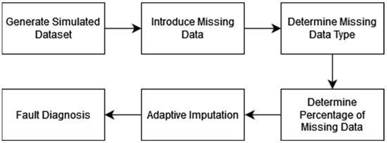
Figure 1.
A block diagram of our methodology.
3.1. Simulated Dataset
The simulated dataset that we constructed for use in our research was designed to realistically reflect data that may be collected by an advanced manufacturing facility. Our generated data simulates the operation of various pieces of machinery in a manufacturing environment, monitored by smart sensors as part of an Internet of Things (IOT) system. The dataset contains a mixture of continuous variables and categorical variables that are commonly used for ML-based CBM tasks.
In our dataset, we simulate data for ten machines over a period of one month, containing 30 days. Sensor readings were collected hourly, resulting in a total of 720 data points per machine, which, given ten machines, means our dataset has a total of 7200 data points. For each machine, three continuous variables were collected: temperature in Celsius (°C), pressure in pascals (Pa), and vibration levels in millimeters per second (mm/s). Two categorical variables were collected: machine status and error code. The machine status variable could contain the following values: “Normal”, “Maintenance Required”, or “Faulty”, while there were 13 possible error codes: “No Error” and “Error A-L”. For each generated error code, specific errors may be associated with certain conditions of the continuous variable. The first row of data for each machine in our simulated dataset is shown in Table 1. The pseudocode for the data generation is given in Algorithm 1.
| Algorithm 1. Synthetic Data Generation |
| 1: numberOfMachines ← 10 2: days ← 30 3: hoursPerDay ← 24 4: numberOfRows ← days × hoursPerDay × numberOfMachines 5: Initialize random seed to 42 6: Generate temperature with normal distribution (μ = 50, σ = 10) of size numberOfRows 7: Generate pressure with uniform distribution (low = 90,000, high = 110,000) of size numberOfRows 8: Generate vibration with normal distribution (μ = 0.5, σ = 0.1) of size numberOfRows 9: Generate timestamps for each hour in days × hoursPerDay, repeat for each machine 10: Generate machines list, repeating each machine name for each timestamp 11: Determine conditions for error codes based on sensor data 12: Assign individual and combined error codes based on conditions 13: Assign status based on error codes: Normal, Maintenance Required, or Faulty |

Table 1.
The first row of data for each machine in our simulated dataset.
As evidenced by the preceding tables, there were 13 possible error codes that could be generated during the synthetic data generation process. The error code that was generated was directly linked to the operational status of the machine that was generated. An error code of “No Error” would trigger an operational status of “Normal”, an error code of “Error A–F” would trigger an operational status of “Maintenance Required”, and an error code “Error G–L” would trigger an operational status of “Faulty”. The logic behind this is that errors A-F are indicative of only a single issue affecting the machine’s condition, while errors G–L occur when multiple issues occur that affect the machine’s condition. The specific operational conditions that lead to each error are shown in Table 2.
Table 2.
Operational conditions leading to each error code in the synthetic dataset.
While the inclusion of the “No Error” and “Error A–F” error codes is fairly self-explanatory given that these codes represent normal operation condition of the machines and then the six possible scenarios of a single issue occurring given our three continuous variables, the inclusion of error codes “Error G–L” warrants further explanation. These error codes represent a combination of different possible issues that may occur. Given the seven error codes indicating normal operating conditions and single issue errors, with three mutually exclusive pairs (ex. ‘Error A’ and ‘Error B’ is not a valid combination because the pressure can’t be simultaneously low and high), there are 23 possible error combinations. For the sake of simplicity, only six of these combinations were included in the logic of the synthetic data generation. The six combinations were selected randomly.
3.2. Introduction of Missing Data
Once we had our synthetic dataset, the next phase of the methodology was to introduce missing data to the dataset. To do this, and to allow each of the three types of missing data to be introduced, we wrote a function in Python to take three parameters: the Pandas DataFrame containing our synthetic data, the type of missing data to add, and the percentage of values to make missing. The pseudocode for this function is shown in Algorithm 2.
| Algorithm 2. Missing Data Introduction |
| Require:df ▷ The original DataFrame Require: type ▷ The type of missing data (MCAR, MAR, or MNAR) Require: percentage ▷ Percentage of missing data to add 1: dfCopy ← df.copy() ▷ Create a copy of the DataFrame 2: featuresToConsider ← [‘Temperature’, ’Pressure’, ’Vibration’] 3: if type = ‘MCAR’ then 4: for feature in featuresToConsider do 5: missingValues ← int(len(dfCopy) × percentage/100) 6: missingIndices ← random choice from dfCopy.index of size missingValues 7: dfCopy.loc[missingIndices] ← NaN 8: end for 9: else if type = ‘MAR’ then 10: highTemperatureIndices ← dfCopy[dfCopy[‘Temperature’] > dfCopy[‘Temperature’].mean()].index 11: MAR_missingVibrationIndices ← random choice from highTemperatureIndices of size int(len(highTemperatureIndices) × percentage/100) 12: dfCopy.loc[MAR_missingVibrationIndices, ‘Vibration’] ← NaN 13: MAR_missingTemperatureIndices ← random choice from highTemperatureIndices of size int(len(highTemperatureIndices) × percentage/100) 14: dfCopy.loc[MAR_missingTemperatureIndices, ‘Temperature’] ← NaN 15: else if type = ‘MNAR’ then 16: highPressureIndices ← dfCopy[dfCopy[‘Pressure’] < dfCopy[‘Pressure’].quantile(0.25)) or dfCopy[‘Pressure’].quantile(0.75))].index 17: highVibrationIndices ← dfCopy[dfCopy[‘Vibration’] < dfCopy[‘Vibration’].quantile(0.25)) or dfCopy[‘Vibration’].quantile(0.75))].index 18: MNAR_missingIndices ← highPressureIndices or highVibrationIndices 19: MNAR_selectedIndices ← random choice from dfCopy[MNAR_missingIndices].index of size int(len(dfCopy(MNAR_missingIndices × percentage/100) 20: dfCopy.loc[MNAR_missingIndices, ‘Pressure’] ← NaN 21: dfCopy.loc[MNAR_missingIndices, ‘Vibration’] ← NaN 22: end if 23: return dfCopy |
The logic of this function can be described as follows:
- Since missing data is classified as MCAR when the missingness has no relationship with any data, observed or missing, if ‘MCAR’ is passed into the ‘type’ parameter, then completely random numerical values are made missing by replacing the existing values with Not a Number (NaN) values.
- Missing data is classified as MAR when the missingness has a relationship with observed data but not with the missing data itself. There were a variety of ways that we could have simulated MAR data for this research, but the method we chose was introduce missing “Vibration” values more frequently when the value in “Temperature” is high, illustrating a systematic relationship between the two variables. In addition to introducing missing “Vibration” values when the temperature is high, we also defined logic to increase the likelihood that there will be missing values in “Temperature”, albeit at a reduced frequency compared to the first case.
- As with MAR data, there were a variety of ways that MNAR data, where missingness is related to the data that’s missing itself, could have been simulated. The method we chose is to introduce missing “Pressure” values more frequently when the values in “Pressure” are considered too low or too high, showing a relationship between “Pressure” with its own values. We also apply this same logic to the values in “Vibration”.
A visualization of the dataset with each of the three types of missing data added is shown in Figure 2.
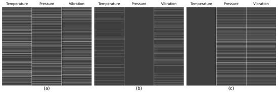
Figure 2.
(a) MCAR data, (b) MAR data, (c) MNAR data. Each type of missing data was introduced with a percentage of 10%. The gray blocks in the figure represent data that is present, and the white lines represent missing data.
3.3. Automatic Determination of the Type of Missing Data
Distinguishing between the different types of missing data programmatically has long proven to be a difficult task. For MCAR data, the randomness implies that there is no pattern or information that can be used to identify the missingness as MCAR without additional external knowledge. Identifying MAR data often involves the use of statistical models that aim to infer relationships between the probability of missingness and other observed variables. The downside to using these models is that they are often complex and laden with assumptions. The types of inferences performed by these statistical models may be difficult to recreate programmatically, because they often involve nuanced judgements that may not be possible without subjective interpretation or additional context about the data, which may include domain-specific knowledge that isn’t always available. MNAR data is generally considered the most complex type of missing data to detect, because understanding why certain data is missing often requires access to the same data that’s unavailable, which makes it almost impossible to identify MNAR data without resorting to making assumptions about the missing data mechanism or obtaining external information.
Additionally, statistical tests designed to identify MCAR data, like Little’s MCAR test, have limitations. They can indicate that the data is not MCAR, but that can’t accurately distinguish between MAR and MNAR without further, more detailed analysis. Creating accurate models for the missing data mechanism, especially to identify MAR and MNAR, requires complex and comprehensive statistical models. These models must consider all observed variables, a task that is not only computationally intensive but also fraught with assumptions that may not accurately reflect the underlying missing data mechanism.
The scheme we used for this research to determine the type of missing data involves the use of the Missingno package for Python. This package enables flexible and easy-to-use missing data visualizations and utilities that all a user to get a quick visual summary of the completeness of a given dataset. Once of the visualizations available in this package is the correlation heatmap, which shows how strongly the presence or absence of one variable affects the presence of another by visualizing the nullity correlation scores for the variables containing missing data. Sample heatmaps of the dataset after each type of missing data has been introduced are shown in Figure 3. Figure 4 is a plot showing how the nullity correlation scores change as the percentage of missing data increases from 1% to 99% for each of the three types of missing data.
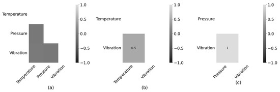
Figure 3.
Correlation heatmaps of the (a) MCAR data, (b) MAR data, and (c) MNAR data. Each heatmap is a visualization of the correlation at 90% missing data.
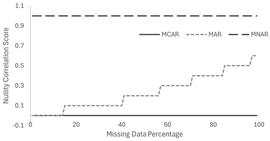
Figure 4.
Nullity correlation scores for each of the three types of missing data as the percentage of missing data increases.
The correlation heatmaps show that there is no correlation score for the MCAR data, which makes sense given that the missingness of MCAR data is completely random and does not depend on the values of any variables observed or unobserved. The moderate correlation score for MAR data also makes sense as in our setup, the missingness in the “Vibration” variable is systematically related to the observed values in “Temperature, but not the unobserved values or its own missing values. The high correlation score found in MNAR data indicates a direct relationship between the missingness of the data and its own values, which in this case represents that both “Pressure” and “Vibration” are more likely to be missing when their values are extreme.
Based on the information depicted in Figure 4, we devised a scheme to automatically determine the type of missing data based on the nullity correlation scores. In our method, if the average correlation score is greater than or equal to 0 but less than 0.1, then the missing data is classified as MCAR. This threshold was selected as missingness in MCAR data is entirely random and does not depend on any observed or unobserved data, meaning that the correlation between missing values and other variables would be very low or non-existent, which is reflected by a nullity correlation threshold of 0.1, which would indicate that any observed correlation is likely due to random chance.
If the average correlation score is between 0.1 and 0.6, then the missing data is classified as MAR. This is because the missingness is related to observed data but not to the missing data itself, resulting in moderate nullity correlation scores because the missingness can be predicted to some extent using the observed variables. If the average correlation score is above 0.6, then the missing data is classified as MNAR. This threshold indicates a strong correlation, capturing the relationship between the data missingness and the values themselves, which is indicative of MNAR data. We evaluated this method for detecting each of the three types of missing data for missing data values between 1 and 99%. The results of this experiment are shown in Table 3.
Table 3.
Accuracy of the missing data classification system.
3.4. Determining the Percentage of Missing Data in a Dataset
To facilitate our adaptive data imputation framework, the system must be able to determine the percentage of missing data in a dataset, as different levels of missing data may necessitate different imputation methods being used to achieve the best results. To ensure our system could do this, we designed a simple method. The pseudocode for this function is given in Algorithm 3.
| Algorithm 3. Calculate missing data percentage |
| Require:df, columns, condition ▷ DataFrame, columns to check, optional condition 1: if condition ≠ None then 2: dfRelevant ← df[condition][columns] 3: else 4: dfRelevant ← df[columns] 5: end if 6: totalCells ← np.product(dfRelevant.shape) 7: missingCells ← dfRelevant.isnull().sum().sum() 8: missingPercentage ← 0 9: if totalCells > 0 then 10: missingPercentage ← (missingCells/totalCells) × 100 11: end if 12: return missingPercentage |
The logic of this function can be described as follows:
- Since we have defined the MAR and MNAR mechanisms as occurring only when data is missing from particular features of the dataset, the function to calculate the percentage of missing data takes a parameter that acts as a filtering condition. If no parameter is provided in the function call, then the missing data scheme defaults to MCAR. If a parameter that specifies the missing data is MAR or MNAR is provided, then the function only considers the relevant rows and columns in the DataFrame for these conditions.
- The determination of the missing data percentage relies on the total number of cells, which is calculated as the product of the dimensions of the DataFrame, and the total number of missing values, determined by summing the count of NaN values across the selected columns.
- The actual calculation to determine the percentage of missing data is calculated by dividing the total number of missing cells by the total number of cells and multiplying by 100 to convert this ratio to a percentage.
- Also included in this function is a safeguard against dividing by zero.
3.5. Adaptive Imputation
Once we were able to automatically assess the missing data percentage, we could begin to implement our adaptive imputation system. Our system is based on the logic that the most effective imputation method for a particular problem can vary based on what type of missing data scheme is present as well as what percentage of the data is missing. Table 4 shows each imputation method that was selected for the types and percentages of missing data. The logic behind these selections will be explained in this subsection.
Table 4.
Outline of the adaptive imputation system.
For MCAR, where the missing data is independent of both observed and unobserved data, the chosen imputation method varies with the percentage of missing data. For small amounts (1–10%), mean imputation is efficient and maintains dataset integrity by replacing missing values with the mean of observed data, preserving the overall dataset’s statistical properties. This method is simple and computationally light, making it ideal for quick fixes in datasets with minimal missing entries. When the missingness is moderate (11–30%), KNN imputation leverages the proximity to the nearest neighbors in the dataset to estimate missing values. This method utilizes the inherent patterns and similarities found in nearby data points to provide a more contextually accurate imputation. As the level of missing data increases (31–50%), MICE becomes particularly advantageous. It iteratively performs multiple regressions, filling in missing values several times to better approximate the inherent uncertainty in the data. For substantial missing data percentages (51–90%), autoencoders, which are neural networks that learn the underlying patterns and structures within data by compressing and decompressing the dataset, can unearth deep correlations, making them particularly effective for reconstructing significantly incomplete datasets.
In MAR scenarios, where the missing data is related to the observed data, the imputation techniques adapt to reflect these dependencies. Even with minimal missing data, MICE proves effective because it can account for the relationships between observed variables and missing data. This robust method enhances the imputation strategy for datasets where missingness depends on observed variables. KNN continues to be a reliable choice for moderate levels of missing data, preserving data integrity by imputing values based on the characteristics of similar observed data. As the percentage of missing data increases, MICE provides a more extensive imputation by analyzing interdependencies within the data, crucial for maintaining the fidelity of more complex datasets. For extensive missing data, autoencoders’ capability to model complex data relationships efficiently makes them invaluable. They reconstruct data based on learned representations, providing a potent tool for detailed and accurate data restoration.
MNAR presents the most challenging scenario, where the missingness depends on unobserved data. Selection models and MIMM are designed to address the specific mechanisms behind MNAR data for small to moderate missing data levels. These methods provide a tailored approach that incorporates assumptions about the reasons behind the missingness into the imputation process, enhancing the accuracy in the presence of biased missing data. For significant levels of missing data, joint modeling utilizes all available data in the estimation process, effectively leveraging both the observed and missing data patterns to make more accurate inferences. For severe missingness, autoencoders’ ability to model complex, non-linear relationships allows them to reconstruct datasets effectively, where traditional methods might not adequately capture the underlying data structure.
3.6. Fault Diagnosis
One of the goals of this paper is to examine the impact that our devised adaptive imputation system has on ML-aided machine fault diagnosis. To do this, we employ the random forest (RF) classifier. RF is a powerful ensemble learning method that can be used for both classification and regression tasks. It functions by combining the outputs of multiple decision trees (DTs) to enhance the model’s predictive accuracy and to avoid overfitting, an issue that is common in models using a single DT.
During the training process for a RF model, multiple DTs are constructed using different subsets of the data and a randomly selected subset of features. This ensures that each DT in the forest is distinct, increasing the overall generalizability of the model. The DTs are not pruned, which allows the model to capture complex data patterns. When RF is being employed in a classification task, the output of the model is determined by a majority vote across all of the DTs.
For fault diagnosis specifically, RF offers significant benefits due to its robustness against noise and its ability to handle large multidimensional datasets, which are typical when dealing with sensor data. RF comes with inherent feature selection capabilities that help manage multicollinearity and enhances the interpretability of the model by evaluating feature important. This is crucial in fault diagnosis, where understanding which sensor readings or operational parameters are most indicative of a fault can lead to more effective predictive maintenance strategies.
4. Results
In this section, the results of our adaptive imputation system and subsequent ML-based fault diagnosis are described. To properly assess performance, the selection of appropriate metrics is important. To evaluate the imputation system, we use the mean absolute error (MAE) and root mean squared error (RMSE). For the fault diagnosis system, we use the accuracy metric. These metrics are defined and the equations are given below.
- MAE—The average of the absolute differences between the predicted values () and the actual values () for a number of observations n.
- RMSE—the square root of the average of the squares of the differences between actual () and predicted () values for a number of observations n.
- Accuracy—the proportion of correct predictions among the total number of predictions.
Table 5 shows the results of the adaptive imputation system across low, moderate, high, and very high levels of missingness. The results are given for 1%, 10%, 11%, 30%, 31%, 50%, 51%, and 90% missing data, the first and last percentage for each interval. For each test, the MAE and RMSE were taken in each individual feature to ensure the most accurate results. For these results, the MAE and RMSE values were normalized against the range of the original data to ensure that the values could be easily presented as a percentage between 0 and 100.
Table 5.
Performance of the adaptive imputation system.
Table 6 reports the accuracy metric for the RF classifier on the full synthetic dataset to provide a baseline to compare against for when the classifier is trained on the imputed dataset. The accuracy is reported for both the ‘Status’ and the ‘Error_Code’ feature, to test the performance of the classifier at identifying two different types of data that is important for fault diagnosis: the condition of the machine and the type of fault itself. Table 7 reports the accuracy of the RF classifier for these two features on missing data percentages of 1%, 10%, 11%, 30%, 31%, 50%, 51%, and 90% for MCAR, MAR, and MNAR data.
Table 6.
Baseline classification results.
Table 7.
Classification results after adaptive imputation.
5. Discussion
From the results shown in Table 5, we can see that for most features and under all missing data mechanisms, the MAE and RMSE increase as the level of missingness increases. This is expected behavior as the more missing data there is, the harder it is to achieve accurate imputation as there is less data to base predictions off of. Between the two error metrics, the RMSE values are consistently higher than the MAE values for the same conditions, reflecting the sensitivity of RMSE to larger errors due to its squaring of error terms.
When data was missing in an MCAR scheme, the temperature feature showed a relatively stable performance up to 50%, after which a significant uptick in the error percentage was observed in both metrics. A continuous increase in error rates as the level of missingness increases is observed for the pressure feature, indicating greater difficulty in imputing the values in this feature accurately under MCAR. For the values in the vibration feature, the error rate actually improved marginally for higher levels of missingness up to 50%, which is an interesting characteristic that warrants further examination.
For MAR, there was an irregular pattern in MAE and RMSE but generally worse performance with very high missingness for the temperature feature, while the vibration feature showcased a slightly more controlled increase in error rates as missingness increased, especially when compared to MCAR. For the pressure feature under an MNAR scheme, the error rates remained somewhat stable across varying levels of missingness, suggesting that the imputation method may be somewhat robust to the MNAR mechanism for this particular feature. The vibration feature showed a gradual increase in error with missingness but starts from a higher baseline at lower missingness levels. Overall, across all of the levels of missingness, the different imputation techniques, and the type of missing data, the pressure feature generally shows the highest rates of errors, suggesting that it may be inherently more difficult to impute accurately compared to temperature and vibration.
Table 6 shows that when no data is missing from the simulated dataset, the RF classifier is extremely accurate at identifying both the operational condition of the machine, as well as the type of fault that is occurring if one is. From Table 7, it is apparent that imputed data where the missing data mechanism was MCAR has the most detrimental effect on the performance of the RF classifier, especially as the percentage of data that was imputed rises. The results show that for missing data percentages of 11%, classifying machine condition and fault type performs relatively well, but at 30% missing data, there is a drastic drop off in terms of classification accuracy, which, despite a mild uptick at 31%, continues as the missing data percentage increases. This accuracy drop off is especially apparent when trying to diagnose the specific type of fault that is occurring, with the lowest accuracy score for values in the “Error_Code” feature being 20.69% compared to 58.55% for the “Status” feature.
Of the three missing data mechanisms, MAR appears to lead to the most consistent results with the least negative impact on classification accuracy. The results show that up until the percentage of missing data gets to 90%, the accuracy of the model does not drop below 90%, and even with the accuracy does drop off at 90% missing data, the model still returns the correct machine condition 83.26% of the time and the correct fault type 82.89% of the time, which is still a reasonable accuracy. As with the classification accuracy under MCAR, the accuracy for the “Error_Code” class is slightly lower than the “Status” class.
The performance of the RF classifier on imputed MNAR data is slightly worse than on MAR data, but is still relatively consistent and accurate, especially compared to MCAR data. The accuracy drops more frequently and at lower percentages of missing data compared to MAR, but it is still reasonable. Like MAR, at 90% missing data especially, the accuracy of classification on the “Error_Code” class is notably lower than that of “Status”, a trend that is consistent across all percentages of missing data.
These results prove that our adaptive imputation system is effective on a simulated dataset specifically designed to reflect realistic data from an advanced manufacturing facility. Although our conclusions discussed in the next section are based on this single simulated dataset, there are several reasons to believe that the proposed method can be successfully applied to other cases. Firstly, our approach is based on well-established imputation techniques and ML algorithms that have been extensively validated in various contexts. Secondly, the adaptive nature of our imputation framework ensures that it can be tailored to the specific characteristics of new datasets, thereby enhancing its generalizability. Additionally, the modular nature of our framework allows for the incorporation of newer and potentially more effective imputation methods as they become available. This ensures that the framework remains relevant and capable of handling future data challenges.
6. Conclusions
Our results demonstrate the effectiveness of ML-based data imputation methods for handling irregularly truncated signals, as well as the effectiveness of a popular ML classifier at correctly identifying the operating condition of a machine, as well as the type of fault if there is a fault present in the machine. Using these methods, we designed an adaptive data imputation system capable of distinguishing between MCAR, MAR, and MNAR data with between 88.85% and 100% accuracy, as well as determining the percentage of missing data present in a simulated dataset. Our system is also capable of switching the ML-based imputation method based on the missing data type and the percentage of missing data.
From our experiments, we found that each of the examined imputation techniques performed reasonably well at imputing the missing data across all missing data mechanisms and percentages of missing data. However, in a simulated example where the dataset consisted of temperature, pressure, and vibration values, the imputation of missing pressure values results in significantly higher MAE and RMSE scores compared to temperature and vibration values, potentially indicating that pressure is an inherently more difficult value to impute compared to temperature and vibration, although it is worth noting that these results were obtained on a simulated dataset, and in order to conclusively claim this, more testing would need to be performed on real-world datasets and under more varied conditions.
Another observation noted from the results is that across each of the three missing data mechanisms, both when evaluating the efficacy of the imputation and the effectiveness of the RF classifier, there is a slight uptick in performance when the percentage of missing data jumps from 30% to 31%. Given that this is a difference of a single percentage point, this uptick seems odd, but this is the point where the adaptive imputation system we designed switches the ML model used for imputation from KNN to MICE for MCAR and MAR data and MIMM to joint modeling for MNAR data, so a potential conclusion could be that KNN and MIMM are more effective at dealing with high levels of missingness compared to MICE and joint modeling. Further experimentation is required to determine if this trend proves true in other scenarios than the one presented in this paper.
There is much potential for future work in this area of research. The adaptive imputation model presented in this paper was designed on a simulated dataset. For deployment to a real-world industrial environment, the methods used would need to revised to fit the characteristics of the data being collected by that organization. One of the pitfalls of current ML research for maintenance-related tasks is that the needs of different organizations can vary greatly. However, one of the benefits of an adaptive imputation system like the one presented in this paper is that if properly and fully implemented in an industrial environment, once the model is trained on the necessary data for that organization, it could prove to be a vital tool for maintenance engineers in ensuring the optimal operating conditions for their equipment.
Another avenue for potential research is to examine even more types of ML models for this task. ML is a vast field of research, and it continues to grow over time, which means that newer, faster, more accurate models are released regularly, each of which could have great benefits for various industries. All in all, ML-based research in the area of CBM is becoming increasingly important as industries turn towards more digital operating processes, and tools such as the adaptive imputation technique described in this paper could greatly enhance operating procedures.
Author Contributions
Conceptualization, K.J.; data curation, T.W.; formal analysis, T.W.; funding acquisition, K.J. and J.O.-M.; investigation, T.W.; methodology, T.W.; project administration, K.J.; resources, K.J. and J.O.-M.; software, T.W.; supervision, K.J.; validation, T.W.; visualization, T.W.; writing—original draft, T.W.; writing—review & editing, K.J. All authors have read and agreed to the published version of the manuscript.
Funding
This research received no external funding.
Data Availability Statement
The raw data supporting the conclusions of this article will be made available by the authors on request.
Conflicts of Interest
The authors declare no conflicts of interest.
References
- Merkt, O. On the Use of Predictive Models for Improving the Quality of Industrial Maintenance: An Analytical Literature Review of Maintenance Strategies. In Proceedings of the 2019 Federated Conference on Computer Science and Information Systems (FedCSIS), Leipzig, Germany, 1–4 September 2019. [Google Scholar] [CrossRef]
- Loukopoulos, P.; Sampath, S.; Pilidis, P.; Zolkiewski, G.; Bennett, I.; Duan, F.; Mba, D. Dealing with missing data for prognostics purposes. In Proceedings of the 2016 Prognostics and System Health Management Conference (PHM-Chengdu), Chengdu, China, 19–21 October 2016. [Google Scholar] [CrossRef]
- Shin, J.-H.; Jun, H.-B. On condition-based maintenance policy. J. Comput. Des. Eng. 2015, 2, 119–172. [Google Scholar] [CrossRef]
- Du, J.; Hu, M.; Zhang, W. Missing data problem in the monitoring system: A review. IEEE Sens. J. 2020, 20, 13984–13998. [Google Scholar] [CrossRef]
- Osman, M.S.; Abu-Mahfouz, A.M.; Page, P.R. A survey on data imputation techniques: Water distribution system as a use case. IEEE Access 2018, 6, 63279–63291. [Google Scholar] [CrossRef]
- Alabadla, M.; Sidi, F.; Ishak, I.; Ibrahim, H.; Affendey, L.S.; Ani, Z.C.; Jabar, M.A.; Bukar, U.A.; Devaraj, N.K.; Muda, A.S.; et al. Systematic review of using machine learning in imputing missing values. IEEE Access. 2022, 10, 44483–44502. [Google Scholar] [CrossRef]
- Rafsunjani, S.; Safa, R.S.; Al Imran, A.; Rahim, M.S.; Nandi, D. An empirical comparison of missing value imputation techniques on APS failure prediction. Int. J. Inf. Technol. Comput. Sci. 2019, 11, 21–29. [Google Scholar] [CrossRef][Green Version]
- Alwan, W.; Ngadiman, N.H.A.; Hassan, A.; Masood, I. Ensemble classifier with missing data in control chart patterns. In Proceedings of the First Australian International Conference on Industrial Engineering and Operations Management, Sydney, Australia, 21–22 December 2022. [Google Scholar] [CrossRef]
- Calabrese, F.; Regattieri, A.; Bortolini, M.; Galizia, F.G. Data-driven fault detection and diagnosis: Challenges and opportunities in real-world scenarios. Appl. Sci. 2022, 12, 9212. [Google Scholar] [CrossRef]
- Rasay, H.; Hadian, S.M.; Naderkhani, F.; Azizi, F. Optimal condition based maintenance using attribute Bayesian control chart. Proc. Inst. Mech. Eng. O J. Risk Reliab. 2023; online first. [Google Scholar] [CrossRef]
- Löwenmark, K.; Taal, C.; Vurgaft, A.; Nivre, J.; Liwicki, M.; Sandin, F. Labelling of annotated condition monitoring data through technical language processing. In Proceedings of the 15th Annual Conference of the Prognostics and Health Management Society (PHM 2023), Salt Lake City, UT, USA, 28 October–2 November 2023. [Google Scholar] [CrossRef]
- Hartini, E. Implementation of missing values handling method for evaluation the system. J. Nucl. React. Technol. 2017, 19, 11–18. [Google Scholar] [CrossRef]
- Martins, A.B.; Fonesca, I.; Farinha, J.T.; Reis, J.; Marques Cardoso, A.J. Prediction maintenance based on vibration analysis and deep learning—A case study of a drying press supported on a hidden Markov model. Appl. Soft Comput. 2024, 163, 111885. [Google Scholar] [CrossRef]
- Appoh, F.; Yunusa-Kaltungo, A. Risk-informed support vector machine regression model for component replacement—A case study of railway flange lubricator. IEEE Access 2021, 9, 85418–85430. [Google Scholar] [CrossRef]
- Song, C.; Zheng, Z.; Liu, K. Building local models for flexible degradation modeling and prognostics. IEEE Trans. Autom. Sci. Eng. 2022, 19, 3483–3495. [Google Scholar] [CrossRef]
- Song, I.; Yang, Y.; Tong, J.I.T.; Ceylan, H.; Cho, I.H. Impacts of fractional hot-deck imputation on learning and prediction engineering data. IEEE Trans. Knowl. Data Eng. 2020, 32, 2363–2373. [Google Scholar] [CrossRef]
- Li, Z.; He, Q. Prediction of railcar remaining useful life by multiple data source fusion. IEEE Trans. Intell. Transp. Syst. 2015, 16, 2226–2235. [Google Scholar] [CrossRef]
- Zhang, Z.W.; Tian, H.-P.; Yan, L.-Z.; Martin, A.; Zhou, K. Learning a credal classifier with optimized and adaptive multiestimation for missing data imputation. IEEE Trans. Syst. Man Cybern. Syst. 2022, 52, 4092–4104. [Google Scholar] [CrossRef]
- Wang, M.; Yang, C.; Zhao, F.; Min, F.; Wang, X. Cost-sensitive active learning for incomplete data. IEEE Trans. Syst. Man Cybern. Syst. 2023, 53, 405–416. [Google Scholar] [CrossRef]
- Ward, T.; Jenab, K.; Ortega-Moody, J. Machine learning models for condition-based maintenance with regular truncated signals. Decis. Sci. Lett. 2024, 13, 192–210. [Google Scholar] [CrossRef]


Disclaimer/Publisher’s Note: The statements, opinions and data contained in all publications are solely those of the individual author(s) and contributor(s) and not of MDPI and/or the editor(s). MDPI and/or the editor(s) disclaim responsibility for any injury to people or property resulting from any ideas, methods, instructions or products referred to in the content. |
© 2024 by the authors. Licensee MDPI, Basel, Switzerland. This article is an open access article distributed under the terms and conditions of the Creative Commons Attribution (CC BY) license (https://creativecommons.org/licenses/by/4.0/).