Abstract
Selective laser melting (SLM) is a rapidly evolving technology that requires extensive knowledge and management for broader industrial adoption due to the complexity of phenomena involved. The selection of parameters and numerical analysis for the SLM process are both costly and time-consuming. In this paper, a three-dimensional radial basis function-finite difference (RBF-FD) meshless model is introduced to accurately and efficiently simulate the molten pool size and temperature distribution during the SLM process for austenitic stainless steel (AISI 316L). Two different volumetric moving heat source models were presented, namely the ray-tracing method heat source model and the double-ellipsoidal shape heat source model. The temperature-dependent material properties and phase change process were also considered, based on experiments and effective models. Results of the model for the molten pool size were validated with those of the literature. The proposed approach can be used to predict the effect of different laser power and scan speed on the molten pool size and temperature gradient along the depth direction. The result reveals that the depth of the molten pool is more sensitive to laser power than scan speed. Under the same scan speed, a 22% change in laser power (45 ± 10 W) affects the maximum temperature proportionally by about 9%. The developed algorithm is computationally efficient and suitable for industrial applications.
1. Introduction
Selective laser melting (SLM), known as direct metal laser melting or laser powder bed fusion, provides significant potential for the direct fabricating of complex three-dimensional structures. Unlike selective laser sintering, SLM involves the complete melting and solidification of metal materials. Various thermal–physical phenomena and morphologies change when a laser beam irradiates the powder layer [1,2]. Initially, part of the powder layer melts when the temperature reaches the melting point as the part has been heated. Subsequently, the molten part solidifies as the temperature falls when the laser beam moves away. During the SLM process, heat transfer mechanisms such as heat conduction between powder particles and heat loss by convection and radiation on the surface are involved. Fluid dynamics such as the surface tension effect, recoil pressure, and the Marangoni convection will occur [3]. Phase transformations, including melting and fusion of powder particles, formation and solidification of the molten pool, and evaporation at the liquid–gas interface, were considered by [4,5]. Boley et al. [6] and Badrossamay and Childs [7] also considered penetration phenomena such as spatial distribution and absorption of laser radiation in the powder. Furthermore, the transient physical behavior during the SLM process is significantly governed by interdependent process parameters: laser-related parameters, scan-related parameters, powder-related parameters, and temperature-related parameters [8].
In practice, the processing parameters applied to a specific case are provided by the material suppliers, obtained through trial procedures and experience. To reduce the cost of the trial process, numerical approaches can be used. Owing to the complexity of the SLM process, many numerical models with approximations and assumptions have been proposed to simplify and avoid time-consuming simulations. Matsumoto et al. [9] used two-dimensional finite element methods for heat conduction and elastic deformation to calculate the temperature and stress distributions of a single metallic layer formed on the powder bed, where the whole area was treated as continuous. Gusarov et al. [10] proposed a model for coupled radiative and conductive heat transfer with an effective volumetric heat source estimated from laser radiation scattering and absorption in a powder layer. Differences in thermal conductivity between the powder bed and dense material were also considered. Hussein et al. [11] provided a non-linear three-dimensional transient model based on a sequentially coupled thermo-mechanical field analysis code developed in the ANSYS parametric design language (APDL). It revealed that the cyclic melting and cooling rates resulted in high von Mises stresses in the product.
Dai and Gu [12] treated the powder bed as a continuum without the effect of discrete powder particles. The formation process of the continuous molten pool, where the thermo-capillary force and the recoil pressure are induced by evaporation, were studied by commercial finite volume method software. Khairallah et al. [13] built fine-scale numerical models with ALE3D, where a laser-ray model was applied, and the powder layer was presumed to be homogeneous bulk materials with effective powder-layer material properties. Tran and Loa [14] proposed a volumetric heat source model that viewed the powder bed as an optical medium, and the laser heat source was assumed to be absorbed gradually along the depth of the powder layer, derived by the Monte Carlo method. A thermal model was developed on Ansys Additive Science to simulate the SLM of a single bead by [15]. The lack of fusion and keyhole defects, which were determined using the calculated melt pool dimensions, were discussed.
In this paper, a transformation is introduced to describe the model of a powder bed and heat source in a coordinate system based on a constant moving heat source instead of a conventional fixed coordinate system. The numerical approach of a meshless method called the radial basis function-generated finite difference (RBF-FD) method [16,17,18] was applied, which has the advantage of solving complex-shaped domains more efficiently while maintaining precision. The resulting model is beneficial to a pre-investigation of the influence of process parameters, including laser power, scanning speed, and spot diameter, on molten pool size in the SLM process.
2. SLM Process Modeling in Moving Coordinate System
2.1. Assumptions
Without losing generality, the assumptions for the complex SLM process are as follows.
- The heat loss from the surface is by radiation and convection only.
- The energy equation of the molten pool is considered in the numerical analysis, but the fluid dynamics are not.
- The material properties are assumed to be temperature dependent. Phase transformation, such as melting and solidification, are discussed through modified thermal properties [1].
- Phenomena such as vaporization, surface tension effect, recoil pressure, and the Marangoni convection are not included in this study.
2.2. Governing Equations
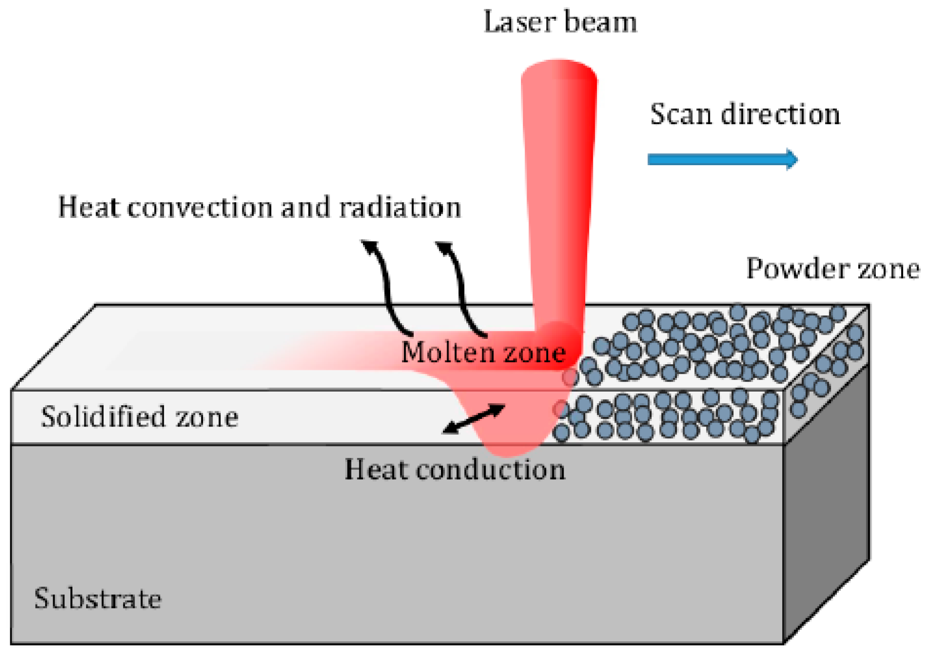
Consider the SLM process shown in Figure 1. An effective volumetric heat source is required instead of surface heat flux on the boundary to accurately predict the size of the molten pool. Moreover, to account for the moving heat source, the coordinate system transforms from the , and fixed coordinate system to the , and coordinate system according to a constant moving heat source by the transformation, as shown in Equation (1)
where is the scan speed of the laser .
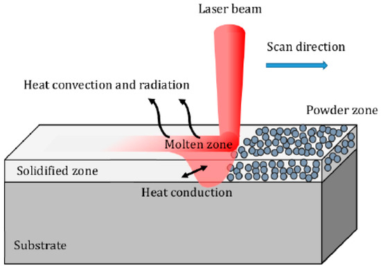
Figure 1.
Schematic diagram of thermal behavior in SLM process.
Using the abovementioned transformation, the three-dimensional heat transfer equation of the system shown in Figure 1 can be rewritten as Equation (2) for the moving coordinate system
where is the material density ; is the heat capacity ; is the time ; , and are the coordinates according to a constant moving heat source ; is the thermal conductivity ; is the volumetric moving heat sources per unit volume and is the current temperature .
2.3. Volumetric Heat Source Models
Heat source models used in the SLM process are based on either the geometrically modified approach or the absorption coefficient profile approach. In the geometrically modified method, different geometric shapes are used to simulate the actual shape of the heat source. On the other hand, the heat source models are not constrained in specific geometries using the absorption coefficient profile approach, where a general form of the heat source is formed by a two-dimensional Gaussian distribution on the top surface while the laser energy is absorbed along the depth of the powder bed based on the absorption coefficient functions.
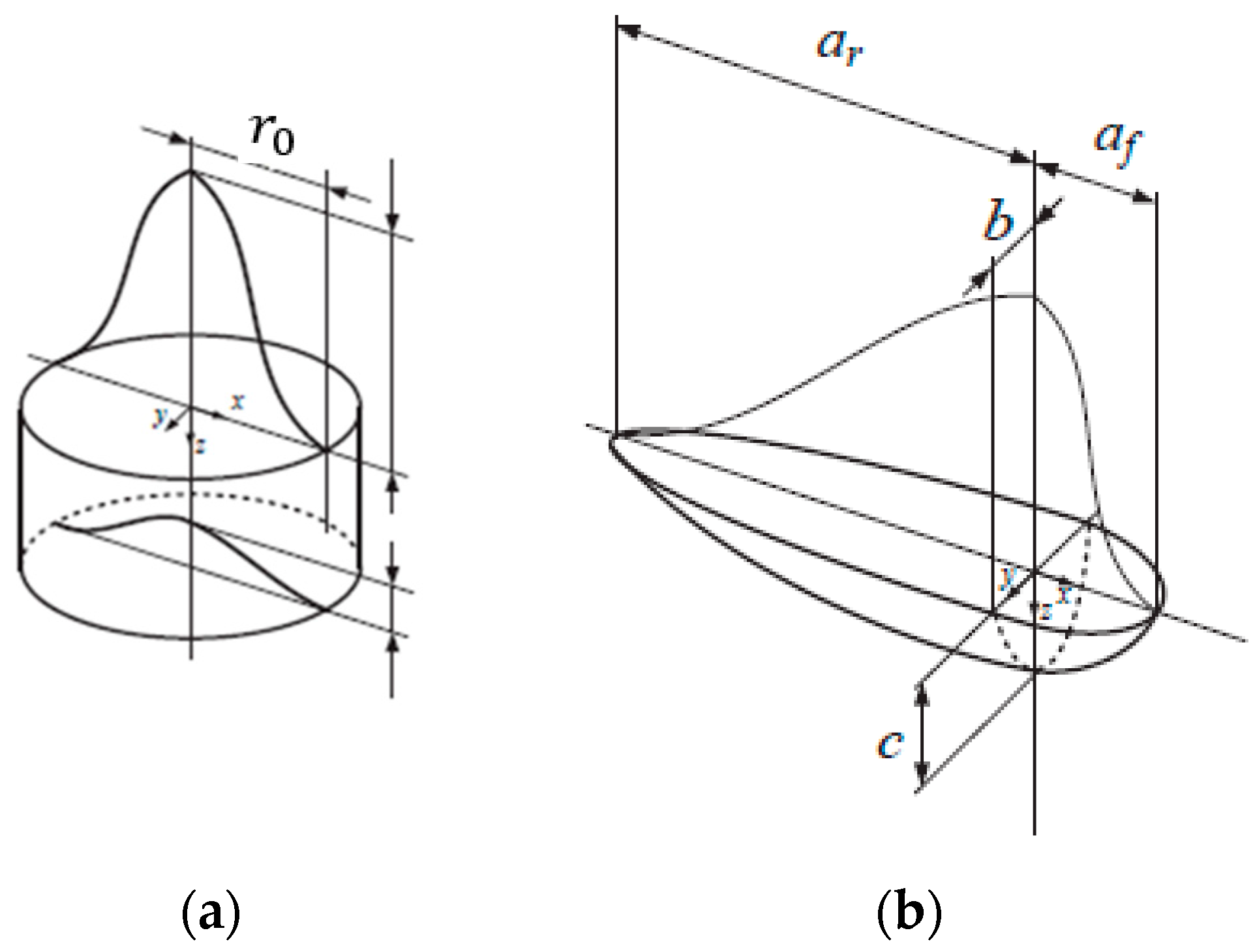
In this study, we will study two types of volumetric heat source models, which are the double-ellipsoidal shape heat source model and the ray-tracing method heat source model, as shown in Figure 2. They belong to the geometrically modified approach and the absorption coefficient profile approach, respectively.
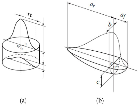
Figure 2.
Schematic diagram of volumetric heat source models. (a) ray-tracing method; (b) double-ellipsoidal shape.
- Ray-tracing method heat source model (I)
The ray-tracing model uses an absorption coefficient profile approach, where the laser energy is absorbed gradually along the depth of the powder bed. This method accounts for the optical properties of the powder bed, leading to a more accurate representation of laser energy distribution within the material. It can capture complex interactions between the laser and the powder, resulting in more precise temperature gradients and molten pool shapes. As shown in Figure 2a, Tran and Loa [14] applied a powder-bed model with randomly distributed particles and calculated the absorption coefficient profile function by Monte Carlo ray-tracing simulations. The volumetric heat source model can be represented as Equation (3) with a moving coordinate system
where is the power of the stationary laser source , is the absorption coefficient function derived by the Monte Carlo ray-tracing simulation, and is the radius of the laser beam .
- Double-ellipsoidal shape heat source model (II)
The double-ellipsoidal shape model uses a geometrically modified approach, where the heat source is represented by a fixed geometric shape (double-ellipsoid). While simpler and computationally efficient, it may not well capture the detailed absorption and scattering effects of the laser within the powder bed. This can lead to less accurate predictions of the temperature distribution and molten pool dimensions. As shown in Figure 2b, the ellipsoidal distribution is introduced by Goldak et al. [19] with semi-axes , and and the center at the reference coordinate origin. The volumetric heat source model can be described as Equation (4) in a moving coordinate system
where , and .
2.4. Initial and Boundary Conditions
The initial condition of the temperature distribution in the powder bed at time is expressed as Equation (5)
where is the ambient temperature and is all the domains.
The boundary conditions at the top surface of the powder bed are expressed as Equation (6), the symmetry surface is expressed as Equation (7), and the other surfaces are expressed as Equation (8)
where is the effective laser heat flux on the top of surface , is the coefficient of the convection , is the Stefan–Boltzmann constant , ε is the emissivity, and is the boundary of .
2.5. Material Properties
- Thermal conductivity
In this study, we used AISI 316L stainless steel as our material. Two states of AISI 316L, the powder state and the solidified state, were considered in this simulation. Gusarov et al. [10] proposed a model to determine the effective thermal conductivity of packed powder beds. They found that the effective thermal conductivity of the powder bed is much smaller than that of bulk material. Therefore, the effective thermal conductivity including phase change in this study is defined as Equation (9)
where is the thermal conductivity of the corresponding bulk material, denotes the packing density of the powder layer, is the average coordination number (note that the coordination number is the number of contact points between a particle and all its surrounding particles), and is the contact size ratio. is the melting temperature, and the phase change is assumed to occur in the temperature between and .
- Density
Similarly, the powder bed can be considered to be a mixture of solid state and gas state. Therefore, the effective density including phase change in this study is expressed as Equation (10)
where is the effective density of the powder bed, is the density of the corresponding bulk material, is the density of gas, and is the porosity, the ratio of the volume occupied by the gas to the total volume of the medium.
- Heat capacity
The effective heat capacity c including phase change in this study can be described as Equation (11)
where and are the heat capacities of the corresponding bulk material and air, respectively.
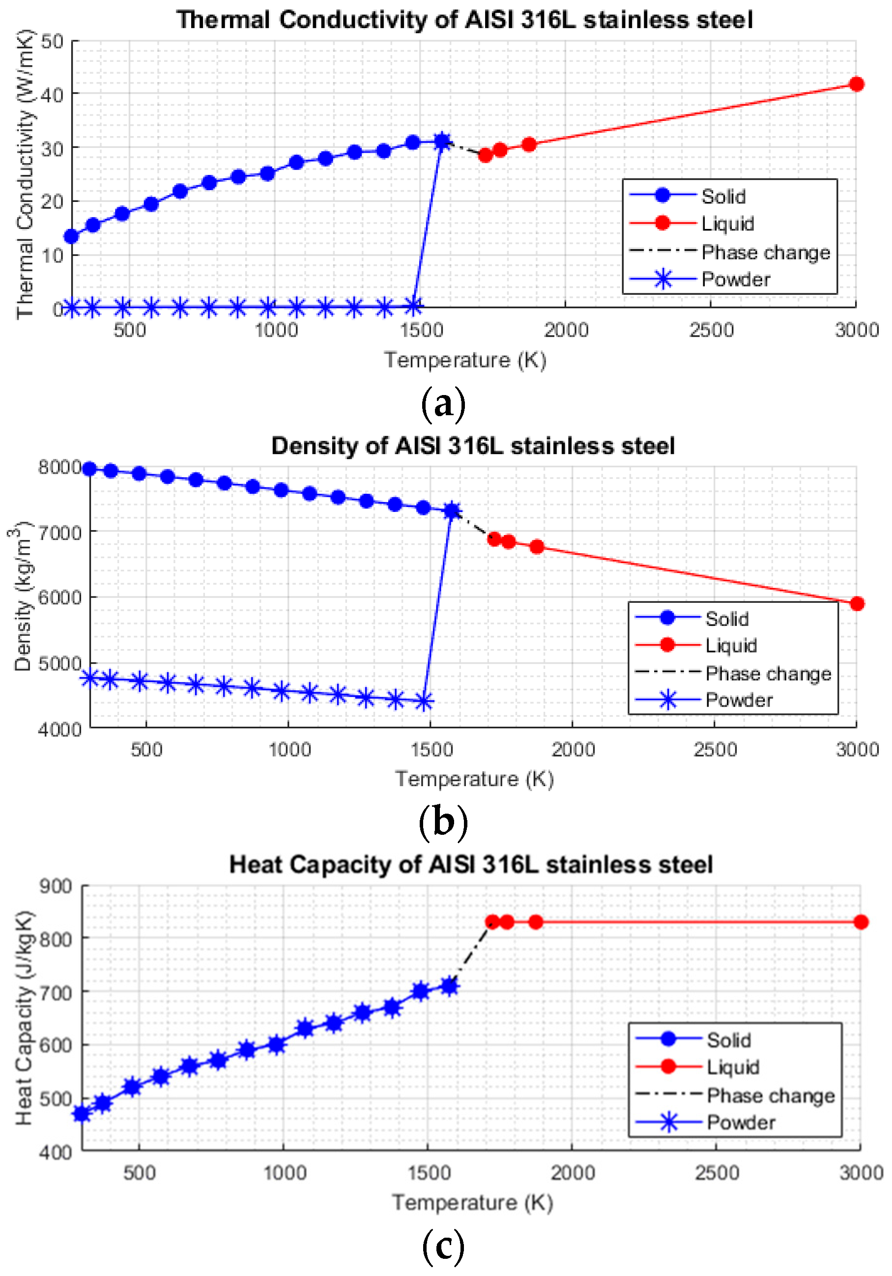
Figure 3 illustrates the data of temperature-dependent material properties of AISI 316L stainless steel. It shows that the effective thermal conductivity and density of the powder bed is much smaller than that of bulk material; however, the effective heat capacity of the powder bed is almost equal to that of the corresponding bulk material.
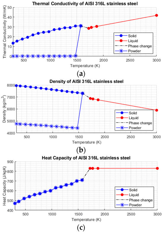
Figure 3.
Thermal material properties of AISI 316L stainless steel. (a) thermal conductivity; (b) density; (c) heat capacity.
A large amount of latent heat will be absorbed or released during the phase change [1], and the thermal material properties will follow Equations (12)–(14)
where the subscript represents phase 1 and phase 2, is the latent heat is a smoothed function to represent the fraction of phase after transition, and is the volumetric content ranging from 0 to 1 during the transition interval, as defined in Equations (15) and (16), respectively
3. Methodology
3.1. RBF-FD Approximations
A typical central finite difference scheme for a derivative of function with respect to at any grid point can be written in the form as follows
where are obtained by using polynomial interpolation or Taylor series expansion.
Instead of using polynomial interpolation or Taylor series expansion, this study applied radial basis function interpolation to obtain the RBF-FD approximation [20,21]. The RBF interpolation can be shown as Equation (18)
where denotes the standard Euclidean 2-norm. is the RBF that can be replaced by any other type in Table 1. is a basis for the space of all d-variate polynomials, and is the shape function, which can be tuned by the user.

Table 1.
Common choices for radial basis function .
Furthermore, the expansion coefficients and are determined by enforcing the conditions as Equations (19) and (20)
According to [18,22], Equation (18) will be well posed without any polynomial augmentation when using some type of RBFs, such as GA, MQ, IMQ, and IQ. However, for the conditionally positive definite RBFs, such as PHS and MQ, polynomial augmentation can be used for Equation (18) to ensure the linear system is uniquely solvable and leads to more accurate results. Therefore, in this study, the RBF of type MQ was applied, and the Lagrange form of the RBF interpolation as Equation (21) was used for deriving the RBF-FD approximation
where satisfies Equation (22),
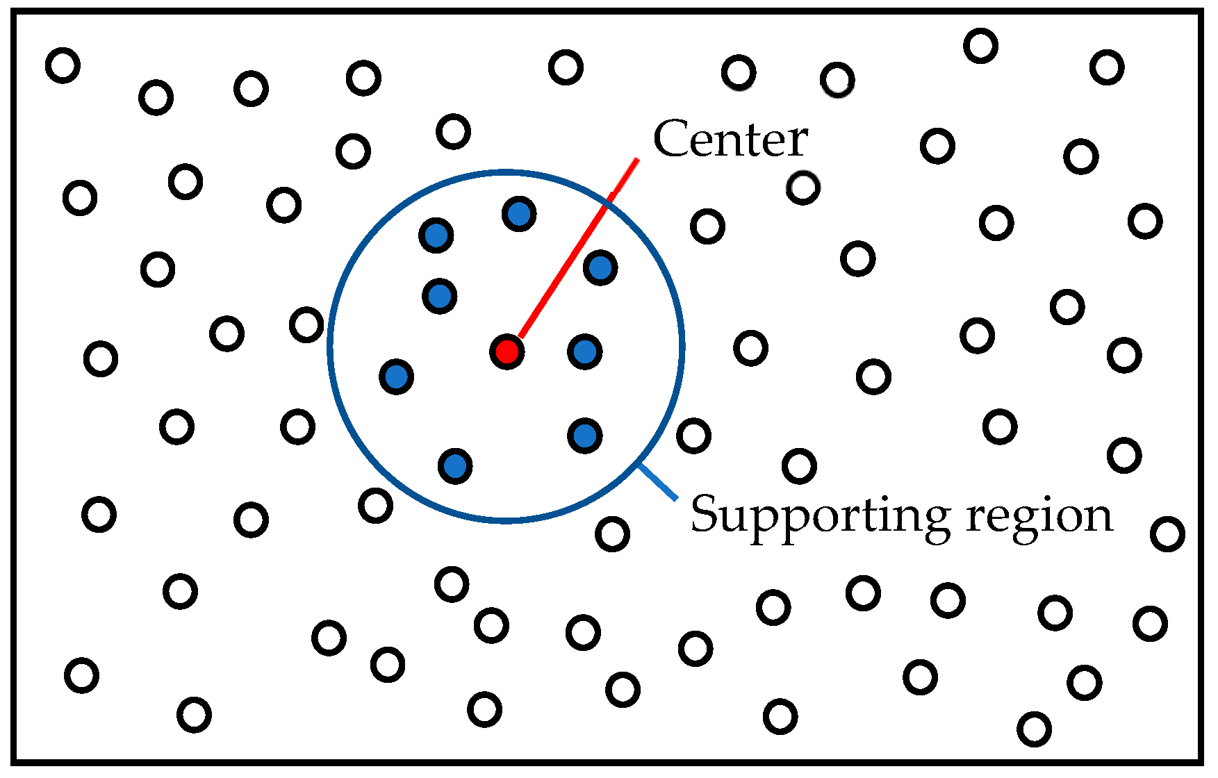
knowing that Equations (18) and (21) infer a global formulation if is the total number of nodes located in the full domain. Therefore, a supporting region is defined first to derive the localized formulation, as shown in Figure 4. It illustrates that the unknown function at any node, say , is approximated by an RBF interpolation with the “center node”, placed on the node itself and the closest surrounding nodes. The nodes constitute the supporting region for the center node.
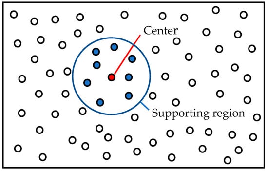
Figure 4.
Schematic diagram of RBF-FD stencil.
In order to match the localized formulation, substitute for in Equation (22) with . Also, the linear differential operator is applied on both sides of Equation (21), and can be described as Equation (23).
According to the finite difference scheme mentioned in Equation (17), this approximation can be rewritten in the form of Equation (24)
where the RBF-FD weights are formally given by the operator applied on the Lagrange form of the RBF, that is, .
Moreover, it has been shown through the literature that better accuracy is gained by adding the constraint as . Hence, the solution for the RBF-FD weights can be determined as Equation (25).
For the conditionally positive definite RBFs such as PHS and MQ, the polynomial terms will be included and (25) can be further represented as (26), where the last entry in the solution vector should be ignored.
It can be seen that the RBF-FD weights solely depend on the relative positioning of the nodes and RBF used. Once these two parameters are defined for a particular problem, the estimation of weights can be performed in the pre-processing stage. Furthermore, as the differential operator can be arbitrary, a similar procedure can be used to obtain the weights for all function derivatives. The convention followed for denoting the weights for any point with supporting points is , , or when the operator is , , or , respectively. For more details on RBF-FD discretization, refer to [23].
3.2. Flow Chart
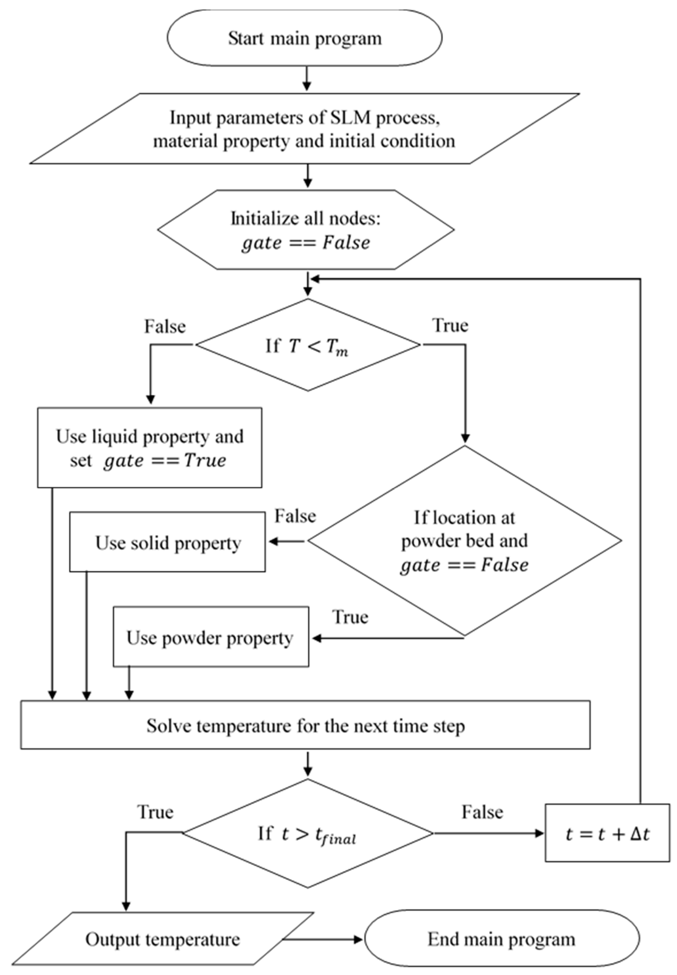
To start the solving procedure, a pre-processing program is required to calculate the RBF-FD weights for all the nodes over the problem domain. After obtaining the weights, the solving procedure can then be carried out, as illustrated in Figure 5. The procedure shows that the phase change among the powder zone, the solidified zone, and the molten zone is irreversible, while the phase change between the substrate and the molten zone is reversible. The “gate” is used to determine whether the powder has been melted. Once the powder is melted and cools down to below the melting temperature, that is, it changes to the solidified zone, it will be simulated with the solid property, not the powder property. Therefore, it can be considered as an irreversible process that is totally different from the substrate.

Figure 5.
Flow chart of the main program.
The advantages of the meshless method are as follows.
- Handling complex geometries: The meshless method can efficiently handle complex-shaped domains without the need for mesh generation, which is often a time-consuming and challenging task in traditional methods like finite element methods (FEM) or finite volume methods (FVM).
- Computational efficiency: It provides a high level of computational efficiency, making it suitable for industrial applications that require fast and accurate simulations.
- Precision: The meshless method maintains a high level of precision in the simulations, even for three-dimensional problems, which is beneficial for predicting the thermal behavior and molten pool size in SLM processes.
- Flexibility: It is easily extendable to various types of problems, including those involving complex boundary conditions and material properties.
- Reduction in numerical artifacts: By avoiding the discretization of the domain into a mesh, the meshless method can reduce the numerical artifacts that may arise from mesh irregularities and improve the overall accuracy of the simulation results.
4. Results and Discussion
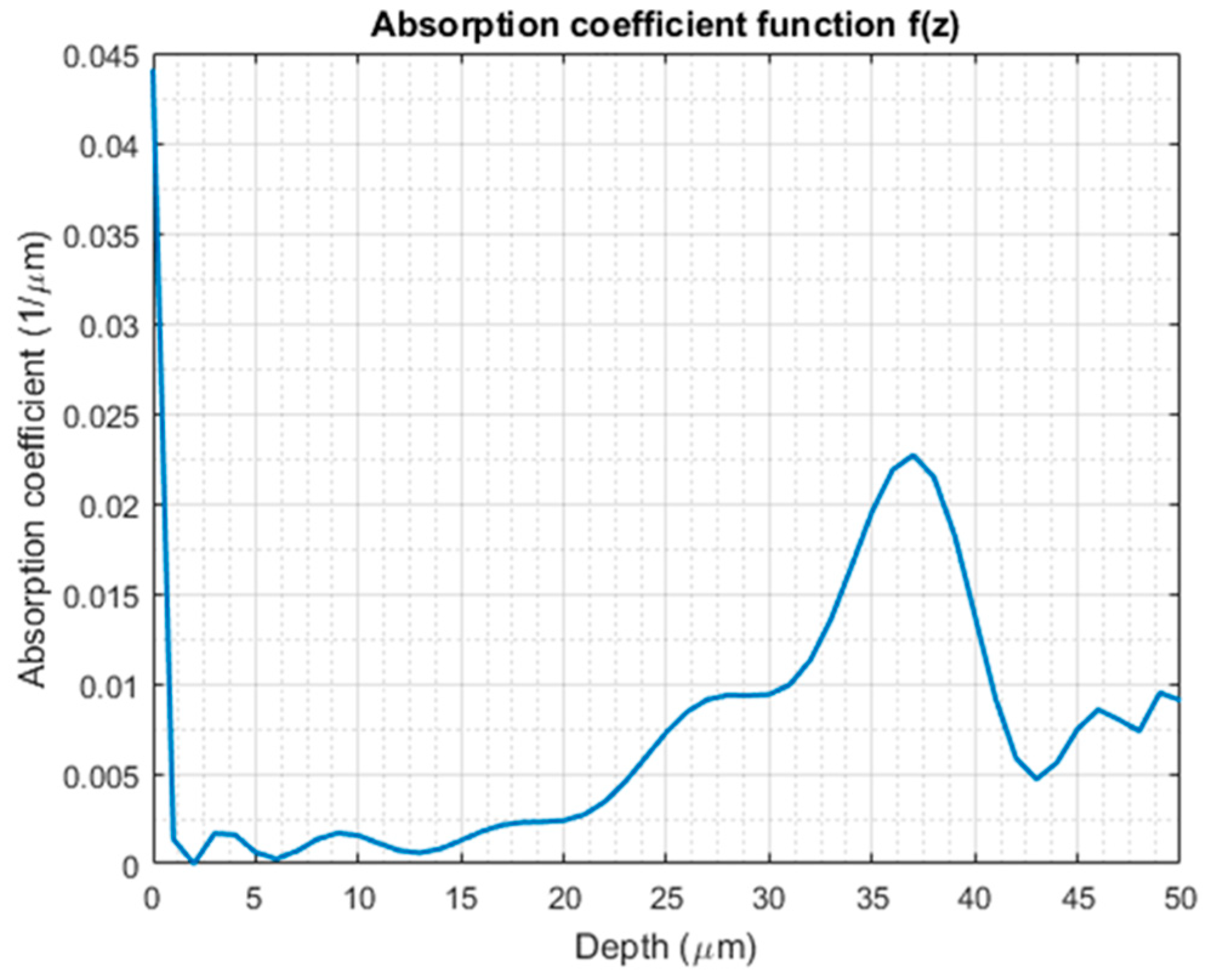
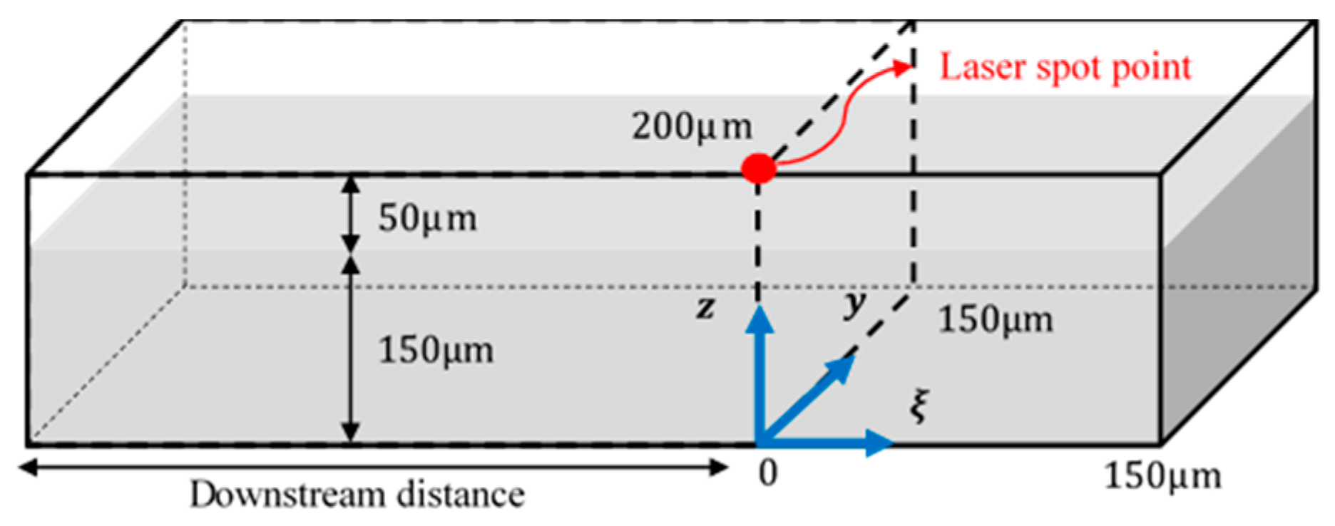
The self-written program of the present study is implemented in Python version 3.6.8 and is executed on an Intel Core™ i7-7700 CPU (Intel Corporation, Santa Clara, CA, USA). All the simulation parameters are listed in Table 2 and Table 3. Figure 6 describes the absorption coefficient function within the powder layer, as determined by Tran and Loa [14]. To compare these two models, the simulation parameters are selected based on delivering the same amount of heat energy to the powder bed with W and . As shown in Figure 7, the geometry of the system is 150 in the direction and 200 in the direction, with 150 upstream for and a sufficiently long distance downstream for .
Table 2.
Simulation parameters with material properties, BCs and IC.
Table 3.
Simulation parameters with two different heat source models.

Figure 6.
Absorption coefficient function for Model 2 from Tran and Loa [14].
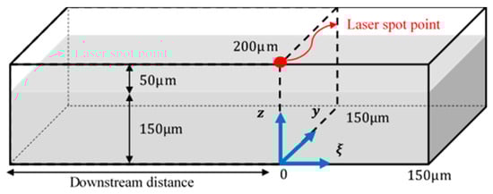
Figure 7.
Geometry of the problem domain.
4.1. Model Validation
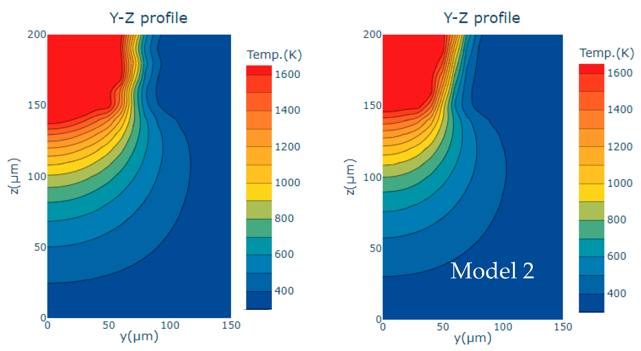
With parameters specified in Table 2 and Table 3, the corresponding cross-sectional temperature distribution of the molten pool is shown in Figure 8. Figure 9 provides a better visualization of the shape and size of the molten pool. It is noted that the maximum temperature of Models 1 and II are 2818 and , respectively. The maximum temperatures and sizes of the molten pool obtained are of a similar scale to those in the literature studies, as shown in Table 4. According to [10], their volumetric heat source was acknowledged to be overestimated, which resulted in a relatively higher maximum temperature of . Moreover, Tran’s simulation model was based on the thermal insulation boundary, meaning that it does not have heat transfer to the outside environment on all surfaces. Both results indicate that the numerical results of this study are reasonable and validated. The proposed approach can be adequately used for thermal analysis of the SLM process.
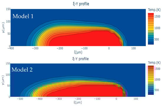
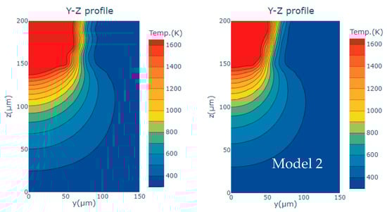
Figure 8.
Cross-sectional temperature distribution with and .
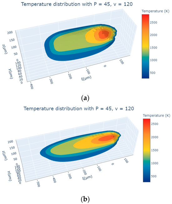
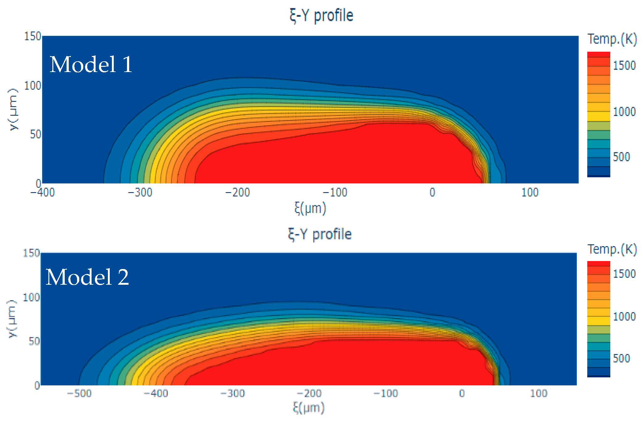
Figure 9.
Temperature distribution with and (a) Model 1; (b) Model 2.
Table 4.
Comparison of the maximum temperature and size of molten pool.
4.2. Temperature Distribution
Understanding the inherent features of SLM processes, such as temperature distribution and molten pool size, is essential before processing. These characteristics influence the physical properties and the overall quality of the resulting products. The effect of laser power and scan speed to temperature distribution along three different directions is shown in Figure 10, Figure 11 and Figure 12.
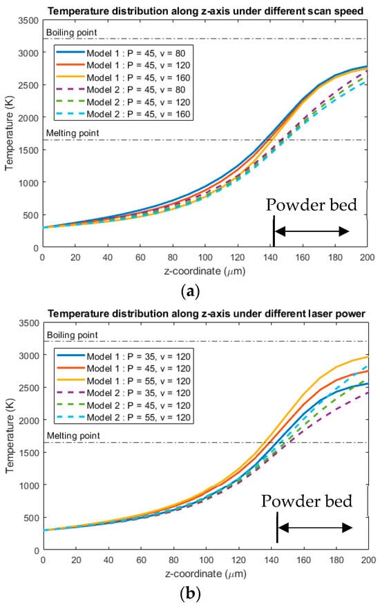
Figure 10.
Temperature distribution along z-axis. (a) Laser power = 45 W; (b) Scan speed = 120 mm/s.
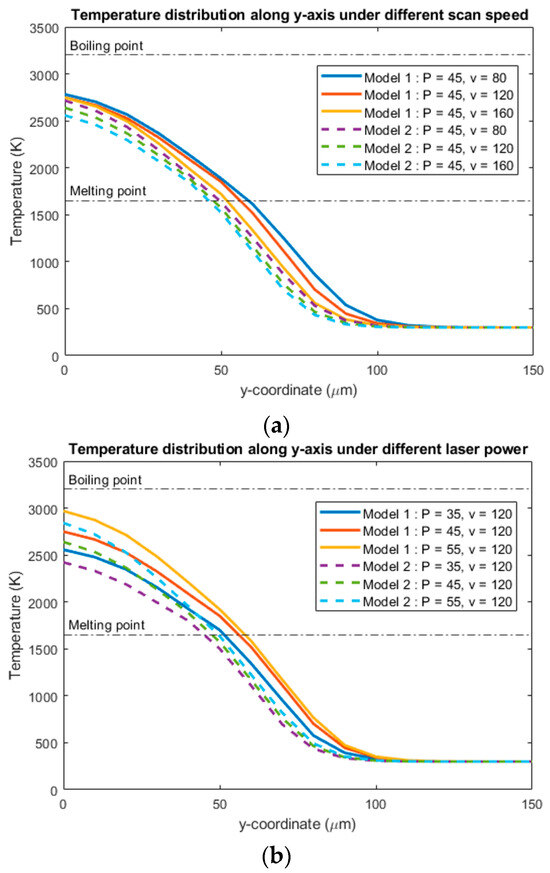
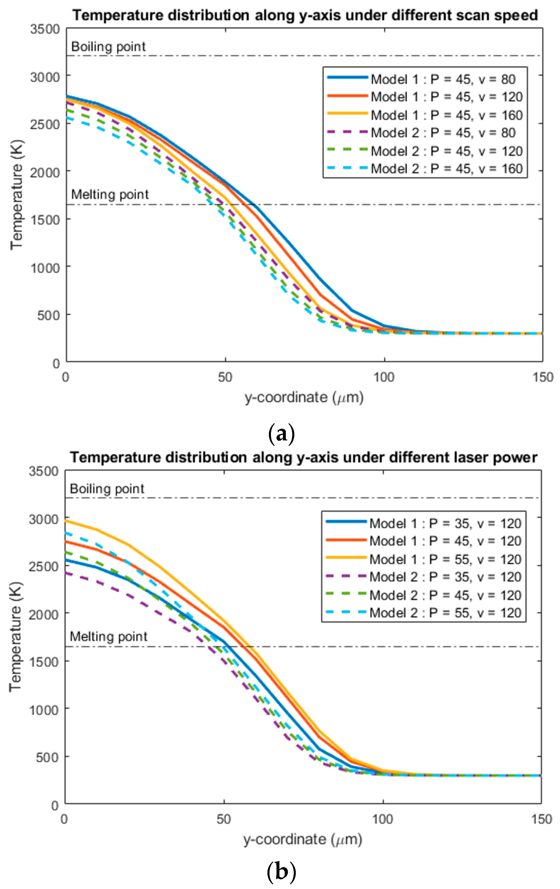
Figure 11.
Temperature distribution along -axis. (a) Laser power = 45 W; (b) Scan speed = 120 mm/s.
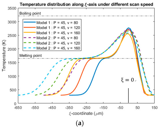
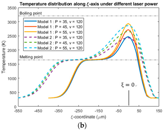
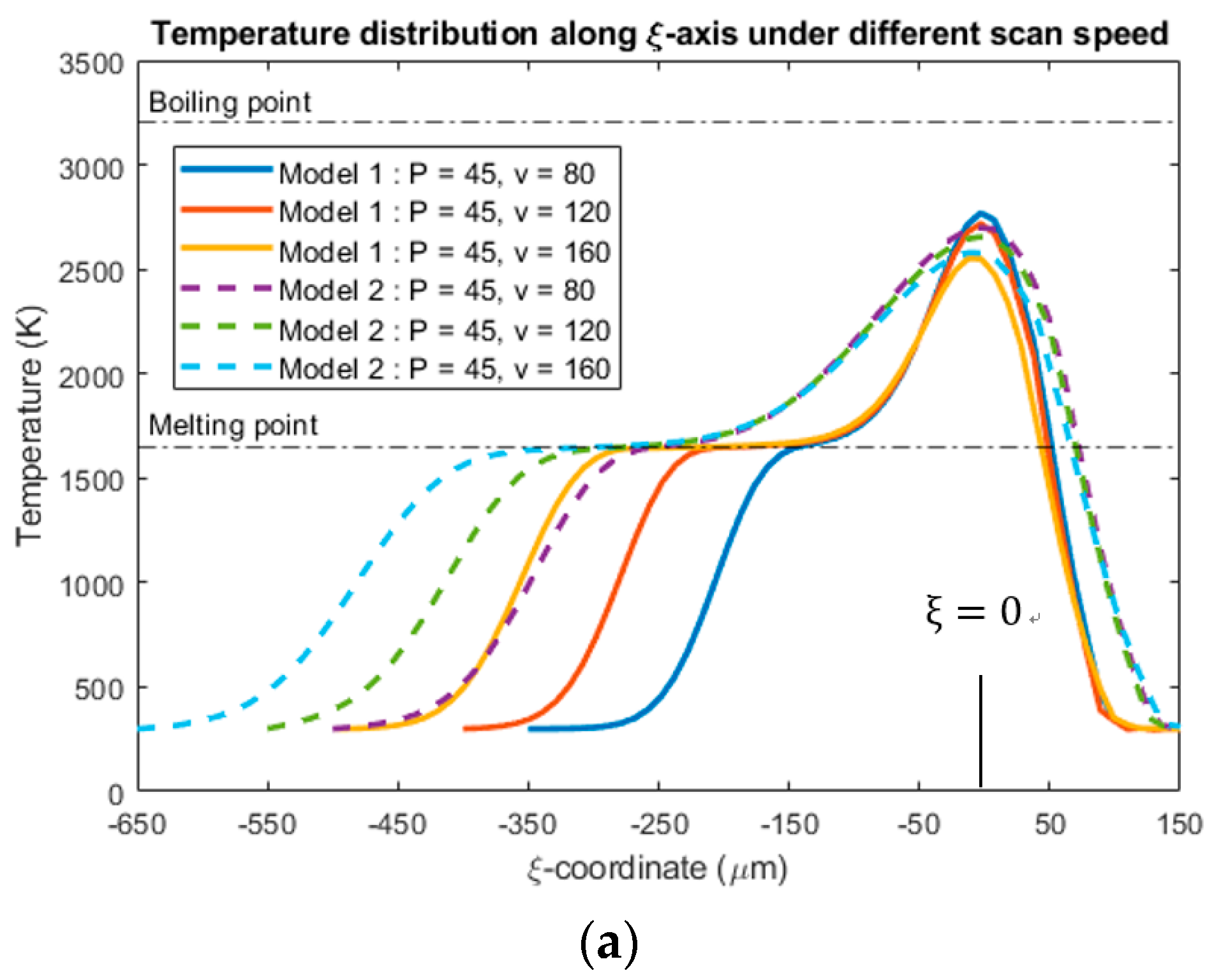
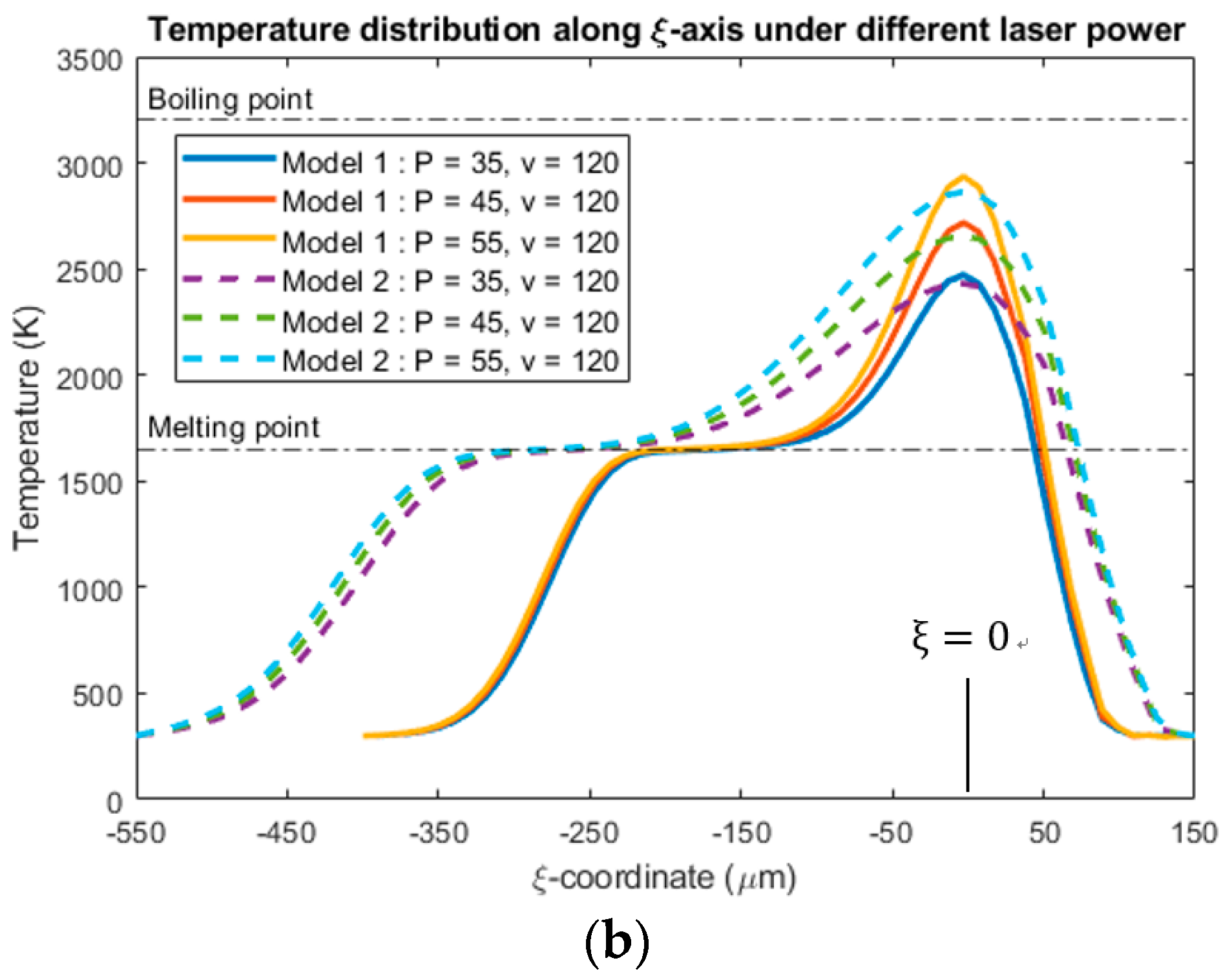
Figure 12.
Temperature distribution along -axis. (a) Laser power = 45 W; (b) Scan speed = 120 mm/s.
Figure 10 shows that the maximum temperature appears at the top of the powder surface, as depicted along the z-axis. This makes sense, since it is the place where the laser beam irradiates. Under the same laser power, a 33% change (±40 mm/s) of scan speed does not significantly change in maximum temperature for Model 1, while the change in maximum temperature for Model 2 is about 10%. Under the same scan speed, a 22% change in laser power (45 ± 10 W) affects the maximum temperature proportionally by about 9%. This reveals that the depth of the molten pool is more sensitive to laser power than scan speed.
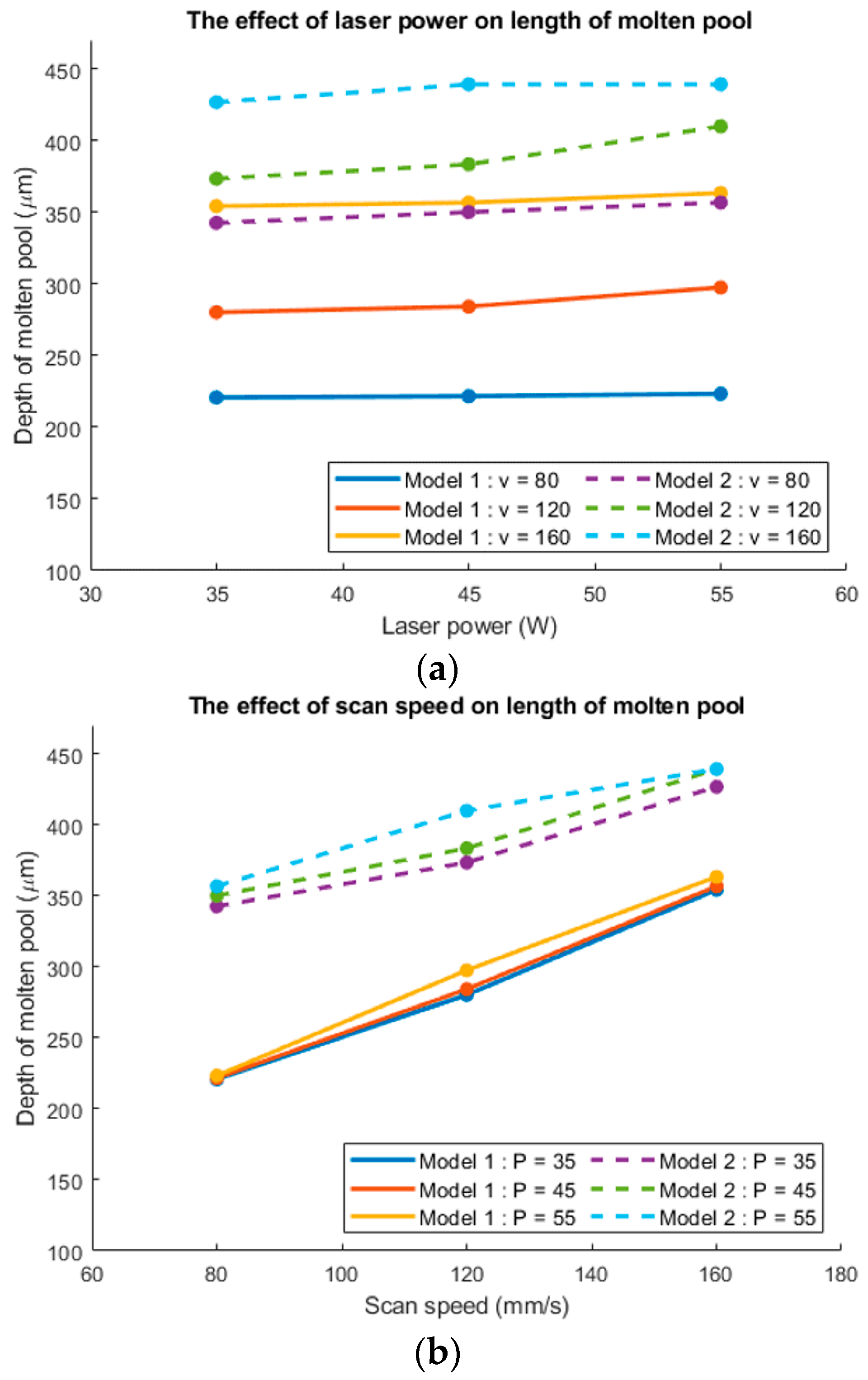
Figure 11 shows that the molten size along the y direction increases with an increase in laser power and a decrease in scan speed, however, not significantly. Figure 12 illustrates the temperature along the -axis. Figure 13 shows the change in pool length along the -axis with different laser power and scan speed. It reveals that an increase in scan speed significantly increases the pool length along the -axis under the same laser power. As the scan speed increases from 80 to 160 , the pool length increases by 26.8% and 12% for heat source Models I and II, respectively. Owing to a similar total heat absorption of the power bed, the corresponding pool width, depth, and maximum temperature decrease.
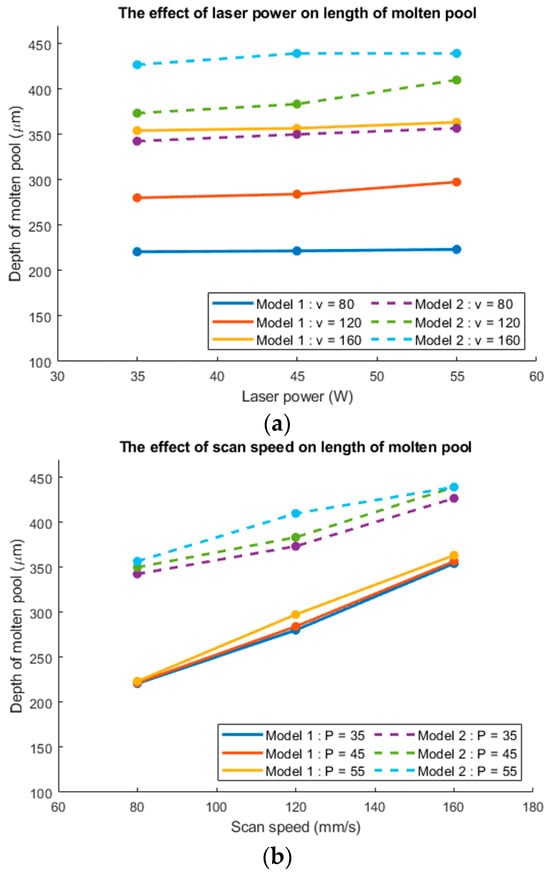
Figure 13.
The effect of laser power and scan speed on molten pool length. (a) The effect of laser power; (b) The effect of scan speed.
Based on the observation that, under the same amount of heat energy, the temperature predicted using Model 1 is much higher than in Model 2, (because the heat source of Model 2 is more widely distributed than Model 1) this causes the predicted temperature to disperse more easily and results in the lower temperature performance.
5. Conclusions
In this paper, three-dimensional models are established to investigate the effect of laser power and scan speed on the thermal behavior during the SLM process. The moving heat source model of double-ellipsoidal shape and the ray-tracing method were applied to study the molten pool shape and size of a stainless steel 316 L powder bed. Furthermore, unlike the previous studies that used the finite element method, this paper applied a meshless method, called RBF-FD, to build a thermal model that is computationally efficient and easy to program.
The numerical results conclude that the length of the molten pool is significantly affected by the scan speed rather than the laser power. The influence on size along the y and z directions is relatively small. The molten pool is larger with the higher laser power and lower scan speed. The temperature distribution along the depth direction increases and is concave from the bottom of the substrate to the junction between the substrate and the powder bed, while it increases and is convex from the junction to the top of the powder bed. Therefore, the maximum temperature gradient is about to 30 for Model 1 and 20 to 25 for Model 2, occurring at the junction between the substrate and the powder bed. However, the mechanical properties of the printed parts by grain structure were not provided in this study; for more on this, refer to the work by Hassine et al. [25].
Author Contributions
Conceptualization, C.-H.W. and C.-K.C.; methodology, C.-K.C. and C.-H.W.; software, C.-H.W.; validation, C.-L.C.; formal analysis, C.-L.C.; data curation, C.-H.W.; writing—original draft preparation, C.-H.W. and C.-L.C.; writing—review and editing, C.-L.C.; supervision, C.-K.C.; funding acquisition, C.-L.C. All authors have read and agreed to the published version of the manuscript.
Funding
This research was funded by the Ministry of Science and Technology, Taiwan, under Grant No. MOST 110-2221-E-006-163.
Institutional Review Board Statement
Not applicable.
Informed Consent Statement
Not applicable.
Data Availability Statement
Data is contained within the article.
Conflicts of Interest
The authors declare no conflict of interest.
References
- Xiang, Z.; Yin, M.; Dong, G.; Mei, X.; Yin, G. Modeling of the thermal physical process and study on the reliability of linear energy density for selective laser melting. Results Phys. 2018, 9, 939–946. [Google Scholar] [CrossRef]
- Duan, X.; Chen, X.; Zhu, K.; Long, T.; Huang, S.; Jerry, F.Y.H. The Thermo-Mechanical Coupling Effect in Selective Laser Melting of Aluminum Alloy Powder. Materials 2021, 14, 1673. [Google Scholar] [CrossRef] [PubMed]
- Wang, D.; Wu, S.; Fu, F.; Mai, S.; Yang, Y.; Liu, Y.; Song, C. Mechanisms and characteristics of spatter generation in SLM processing and its effect on the properties. Mater. Des. 2017, 117, 121–130. [Google Scholar] [CrossRef]
- Kruth, J.-P.; Levy, G.; Klocke, F.; Childs, T.H.C. Consolidation phenomena in laser and powder-bed based layered manufacturing. CIRP Ann. 2007, 56, 730–759. [Google Scholar] [CrossRef]
- FVerhaeghe, F.; Craeghs, T.; Heulens, J.; Pandelaers, L. A pragmatic model for selective laser melting with evaporation. Acta Mater. 2009, 57, 6006–6012. [Google Scholar] [CrossRef]
- Boley, C.D.; Khairallah, S.A.; Rubenchik, A.M. Calculation of laser absorption by metal powders in additive manufacturing. Appl. Opt. 2015, 54, 2477–2482. [Google Scholar] [CrossRef] [PubMed]
- Badrossamay, M.; Childs, T.H.C. Further studies in selective laser melting of stainless and tool steel powders. Int. J. Mach. Tools Manuf. 2007, 47, 779–784. [Google Scholar] [CrossRef]
- Gibson, I.; Rosen, D.W.; Stucker, B. Additive Manufacturing Technologies; Springer: Berlin/Heidelberg, Germany, 2010. [Google Scholar]
- Matsumoto, M.; Shiomi, M.; Osakada, K.; Abe, F. Finite element analysis of single layer forming on metallic powder bed in rapid prototyping by selective laser processing. Int. J. Mach. Tools Manuf. 2002, 42, 61–67. [Google Scholar] [CrossRef]
- Gusarov, A.V.; Yadroitsev, I.; Bertrand, P.; Smurov, I. Model of radiation and heat transfer in laser-powder interaction zone at selective laser melting. J. Heat Transf. 2009, 131, 072101. [Google Scholar] [CrossRef]
- Hussein, A.; Hao, L.; Yan, C.; Everson, R. Finite element simulation of the temperature and stress fields in single layers built without-support in selective laser melting. Mater. Des. 1980–2015 2013, 52, 638–647. [Google Scholar] [CrossRef]
- Dai, D.; Gu, D. Tailoring surface quality through mass and momentum transfer modeling using a volume of fluid method in selective laser melting of TiC/AlSi10Mg powder. Int. J. Mach. Tools Manuf. 2015, 88, 95–107. [Google Scholar] [CrossRef]
- Khairallah, S.A.; Anderson, A.T.; Rubenchik, A.; King, W.E. Laser powder-bed fusion additive manufacturing: Physics of complex melt flow and formation mechanisms of pores, spatter, and denudation zones. Acta Mater. 2016, 108, 36–45. [Google Scholar] [CrossRef]
- Tran, H.-C.; Loa, Y.-L. Heat transfer simulations of selective laser melting process based on volumetric heat source with powder size consideration. J. Mater. Process. Technol. 2018, 255, 411–425. [Google Scholar] [CrossRef]
- Slama, M.B.; Chatti, S.; Hassine, N.; Kolsi, L. Numerical investigation of the melt pool geometry evolution during selective laser melting of 316L SS. Matériaux Tech. 2024, 112, 208. [Google Scholar] [CrossRef]
- Tolstykh, A.I.; Shirobokov, D.A. On using radial basis functions in a “finite difference mode” with applications to elasticity problems. Comput. Mech. 2003, 33, 68–79. [Google Scholar] [CrossRef]
- Shu, C. Local radial basis function-based differential quadrature method and its application to solve two-dimensional incompressible Navier-Stokes equations. Comput. Methods Appl. Mech. Eng. 2003, 192, 941–954. [Google Scholar] [CrossRef]
- Wright, G.B.; Fornberg, B. Scattered node compact finite difference-type formulas generated from radial basis functions. J. Comput. Phys. 2006, 212, 99–123. [Google Scholar] [CrossRef]
- Goldak, J.; Chakravarti, A.; Bibby, M. A new finite element model for welding heat sources. Metall. Trans. B 1984, 15, 299–305. [Google Scholar] [CrossRef]
- Sundin, U. Global Radial Basis Function Collocation Methods for PDEs. Licentiate Thesis, Uppsala University, Uppsala, Sweden, 2019. [Google Scholar]
- Pooladi, F.; Larsson, E. Stabilized interpolation using radial basis functions augmented with selected radial polynomials. J. Comput. Appl. Math. 2024, 437, 115482. [Google Scholar] [CrossRef]
- Fornberg, B.; Larrson, E.; Flyer, N. Stable computations with Gaussian radial basis functions. Siam J. Sci. Comput. 2011, 33, 869–892. Available online: http://n2t.net/ark:/85065/d7zp47fz (accessed on 23 July 2024). [CrossRef]
- Bayona, V.; Flyer, N.; Fornberg, B. On the role of polynomials in RBF-FD approximations: III. Behavior near domain boundaries. J. Comput. Phys. 2019, 380, 378–399. [Google Scholar] [CrossRef]
- ISO/ASTM 52900:2021; Additive Manufacturing—General Principles—Terminology, Fundamentals and Vocabulary. International Organization for Standardization: Geneva, Switzerland, 2021. Available online: https://www.iso.org/standard/74514.html (accessed on 23 July 2024).
- Hassine, N.; Chatti, S.; Kolsi, L. Tailoring grain structure including grain size distribution, morphology, and orientation via building parameters on 316L parts produced by laser powder bed fusion. Int. J. Adv. Manuf. Technol. 2024, 131, 4483–4498. [Google Scholar] [CrossRef]


Disclaimer/Publisher’s Note: The statements, opinions and data contained in all publications are solely those of the individual author(s) and contributor(s) and not of MDPI and/or the editor(s). MDPI and/or the editor(s) disclaim responsibility for any injury to people or property resulting from any ideas, methods, instructions or products referred to in the content. |
© 2024 by the authors. Licensee MDPI, Basel, Switzerland. This article is an open access article distributed under the terms and conditions of the Creative Commons Attribution (CC BY) license (https://creativecommons.org/licenses/by/4.0/).