Real-Time Calculation of CO₂ Conversion in Radio-Frequency Discharges under Martian Pressure by Introducing Deep Neural Network

Abstract

In recent years, the in situ resource utilization of ${\mathrm{CO}}_2$ in the Martian atmosphere by low-temperature plasma technology has garnered significant attention. However, numerical simulation is extremely time-consuming for modeling the complex ${\mathrm{CO}}_2$ plasma, involving tens of species and hundreds of reactions, especially under Martian pressure. In this study, a deep neural network (DNN) with multiple hidden layers is introduced to investigate the ${\mathrm{CO}}_2$ conversion in radio-frequency (RF) discharges at a given power density under Martian pressure in almost real time. After training on the dataset obtained from the fluid model or experimental measurements, the DNN shows the ability to accurately and efficiently predict the various discharge characteristics and plasma chemistry of RF ${\mathrm{CO}}_2$ discharge even in seconds. Compared with conventional fluid models, the computational efficiency of the DNN is improved by nearly ${10}^6$ times; thus, a real-time calculation of RF ${\mathrm{CO}}_2$ discharge can almost be achieved. The DNN can provide an enormous amount of data to enhance the simulation results due to the very high computational efficiency. The numerical data also suggest that the ${\mathrm{CO}}_2$ conversion increases with driving frequency at a fixed power density. This study shows the ability of the DNN-based approach to investigate ${\mathrm{CO}}_2$ conversion in RF discharges for various applications, providing a promising tool for the modeling of complex non-thermal plasmas.

1. Introduction

With the expansion of Mars exploration, the utilization of local resources on Mars to produce mission-critical consumables for Mars exploration, such as propellants and life-support consumables, has gained widespread attention [1,2,3]. Carbon dioxide (${\mathrm{CO}}_2$), the most abundant component of the Martian atmosphere (96%), can be used as the prime source for in situ resource utilization (ISRU) to produce carbon monoxide (CO) and oxygen (${\mathrm{O}}_2$). The carbon monoxide can be collected to manufacture rocket vehicles, and the oxygen can be made available for breathing [4,5]. In addition, ${\mathrm{CO}}_2$ is a major source of carbon and oxygen and can be used for the in situ manufacturing of plastics and other organic compounds. However, the thermodynamic stability of ${\mathrm{CO}}_2$ molecules is the major challenge to the ISRU of ${\mathrm{CO}}_2$ on Mars. In recent years, non-thermal plasmas (NTPs) have become a widely discussed topic in many fields due to their unique advantages [6,7,8]. NTP is an efficient gas-activation approach maintained by electrical discharges, which allow the energetic electrons to coexist with relatively cold gas molecules. The energy stored in energetic electrons can offer a unique way to break the strong C=O bond [9,10]. More significantly, the low pressure (∼600 Pa) and low temperature (∼210 K) of the Martian atmosphere are considered to be the ideal conditions for the local splitting of ${\mathrm{CO}}_2$ using NTPs [11,12]. Currently, extensive numerical and experimental investigations are performed to achieve the splitting of ${\mathrm{CO}}_2$ using dielectric barrier discharges [13,14], gliding arc discharges [15,16], microwave discharges [17,18], and radio-frequency (RF) discharges [19,20,21]. Among the plasma sources mentioned above, RF discharges are distinguished by higher electron density, especially operating in the low-pressure and low-temperature environment on Mars [22]. RF discharge, therefore, offers a promising avenue for the ISRU of ${\mathrm{CO}}_2$ on Mars. However, as the input power increases, the homogenous RF plasma may transform into a radially contracting plasma with a high gas temperature, with the possible risk of damaging the electrodes. Previous research has demonstrated that RF discharges could exhibit higher stability with increasing driving frequency [23,24].

As a complementary method to experimental diagnosis, numerical simulations can overcome the experimental limitations and provide insight into the discharge properties and plasma chemistry of RF ${\mathrm{CO}}_2$ plasma. The zero-dimensional kinetic model is widely used to describe the behaviors of various plasmas due to its high computational efficiency, but the spatial properties, such as the distributions of the electric field and the profiles of the product particles, are not available [25,26]. The fluid model is able to obtain the spatial distributions of plasma species and the electric field with relatively high computational efficiency, which has received more attention in simulating ${\mathrm{CO}}_2$ conversion [27,28,29]. Unfortunately, on the one hand, ${\mathrm{CO}}_2$ plasma is a multi-scale system with significant differences in the lifetimes of different plasma species; on the other hand, plasma species under Martian pressure are characterized by large transport rates. To accurately describe the behaviors of different species, the fluid model should adopt fine time steps and spatial meshes, which significantly increases the computational load of the fluid model. In addition, in order to accurately describe the driving frequency effect in RF ${\mathrm{CO}}_2$ plasma, a given power density should be chosen to eliminate the influence of other discharge parameters [30]. However, it is challenging to precisely meet the given power density at all driving frequencies in the numerical simulation. The interpolation method is often adopted to approximate a given power density, which inevitably introduces errors and may even distort the evolutions of some essential properties, especially in violent discharges [31]. Therefore, a more efficient method should be developed to quickly and accurately describe the ${\mathrm{CO}}_2$ conversion in RF discharges under Martian pressure at a given power density.

In recent years, with the development of machine learning, data-driven models, such as artificial neural networks (ANNs) and deep neural networks (DNNs), have been introduced into the studies of low- temperature plasmas [32,33]. Compared to ANNs, DNNs can extract abstract high-level features and produce accurate predictions in complex chemical, physical, and biological systems [34,35,36]. To better understand the underlying physical and chemical properties of plasma, considerable effort has been devoted to applying DNNs to various plasma processes. Garola et al. [37] investigated the possibility of DNNs for integrating diagnostic data in the active control of fusion-relevant plasmas in complex scenarios. Based on a DNN, Liu et al. [38] developed a microwave interferometry method for time-varying plasmas, and the DNN was used to effectively eliminate the noise and accurately diagnose the time-varying electron density and collision frequency. The dielectric barrier discharges driven by sinusoidal or pulsed voltages can also be calculated by the optimized DNN models [39,40]. A neural network was constructed to investigate the effects of chamber size, gas flow rate, and input power on ${\mathrm{CO}}_2$ conversion in a DBD reactor [41], and the results showed that neural networks have great potential for evaluating and predicting the performance of plasma-assisted ${\mathrm{CO}}_2$ conversion. More critically, the studies in Refs. [42,43] showed that DNNs could offer mesh-less implementations for modeling multi-physics and multi-scale systems. It is, therefore, feasible to model and predict the discharge characteristics and plasma chemistry of RF ${\mathrm{CO}}_2$ discharge under Martian pressure using DNNs.

In this paper, a DNN is constructed based on the characteristics of RF ${\mathrm{CO}}_2$ discharges and trained using simulation data obtained from the fluid model, and then, this DNN is employed to describe the discharge characteristics and plasma chemistry of RF ${\mathrm{CO}}_2$ discharges with various driving frequencies and input power densities. The second section is concerned with the methodology used for this study, including the descriptions of the fluid model and the DNN algorithm. The third section begins by illustrating the validity and efficiency of DNN prediction by comparing the prediction results with the fluid simulation results, and then, the well-trained DNN is applied to investigate the effects of driving frequency and input power density on the ${\mathrm{CO}}_2$ conversion in RF discharges under Martian pressure, which further indicates that the DNN is capable of obtaining enough prediction results based on the limited training data. Finally, a summary is given.

2. Description of Methodology

2.1. Description of Fluid Model

In this paper, the RF ${\mathrm{CO}}_2$ discharge is ignited between two parallel plate electrodes with an electrode spacing of 2 mm, and the electrode gap is filled with ${\mathrm{CO}}_2$ gas at a Martian pressure of 4.5 Torr. Based on Martian conditions, 26 species were selected using a zero-dimensional kinetic model [44]. These plasma species in this model include seven charged species (electron, ${\mathrm{O}}^{-}$, ${\mathrm{O}}_2^{-}$, ${\mathrm{CO}}_3^{-}$, ${\mathrm{CO}}_4^{-}$, ${\mathrm{CO}}_2^{+}$, and ${\mathrm{O}}_2^{+}$), five neutral species (CO, C, O, ${\mathrm{O}}_2$, and ${\mathrm{O}}_3$), 13 excited species (${\mathrm{CO}}_2{\mathrm{e}}_1$, ${\mathrm{CO}}_2{\mathrm{v}}_{\mathrm{a}}$, ${\mathrm{CO}}_2{\mathrm{v}}_{\mathrm{b}}$, ${\mathrm{CO}}_2{\mathrm{v}}_{\mathrm{c}}$, ${\mathrm{CO}}_2{\mathrm{v}}_{1\mathrm{a}}$, ${\mathrm{CO}}_2{\mathrm{v}}_1$, ${\mathrm{CO}}_2{\mathrm{v}}_2$, ${\mathrm{CO}}_2{\mathrm{v}}_3$, ${\mathrm{CO}}_2{\mathrm{v}}_4$, ${\mathrm{CO}}_2{\mathrm{v}}_5$, ${\mathrm{CO}}_2{\mathrm{v}}_6$, ${\mathrm{CO}}_2{\mathrm{v}}_7$, and ${\mathrm{CO}}_2{\mathrm{v}}_8$), and the dominant background gas ${\mathrm{CO}}_2$. The chemical reactions in ${\mathrm{CO}}_2$ plasma and the corresponding reaction coefficients were obtained from the previous study in Ref. [44].

The simulation results obtained from the fluid model were used as the data source for training the DNN, and the effectiveness of this fluid model was verified in Ref. [45] by comparing with the experimental measurements. The governing equations in this fluid model include the continuity equations with drift–diffusion approximation, the Poisson equation, and the electron energy conservation equation as follows [46,47,48]:

$${\displaystyle \frac{\partial n_i}{\partial t}}+{\displaystyle \frac{\partial {\Gamma }_i}{\partial x}}=R_i$$

(1)

$${\Gamma }_i=q_i{\mu }_i{n}_{i}E-D_i{\displaystyle \frac{\partial n_i}{\partial x}}$$

(2)

$${\displaystyle \frac{\partial E}{\partial x}}={\displaystyle \frac{\rho }{{\epsilon }_0}}$$

(3)

$${\displaystyle \frac{\partial }{\partial t}}\left({\displaystyle \frac{3}{2}}{k}_{\mathrm{B}}{n}_{\mathrm{e}}{T}_{\mathrm{e}}\right)=-{\displaystyle \frac{\partial Q_{\mathrm{e}}}{\partial x}}-e_0\sum _j\mathsf{\Delta }{E}_j{k}_j-e_0{\Gamma }_{\mathrm{e}}E-3k_{\mathrm{B}}{n}_{\mathrm{e}}{\displaystyle \frac{m_{\mathrm{e}}}{m_{\mathrm{gas}}}}\left(T_{\mathrm{e}}-T_{\mathrm{gas}}\right)\overline{{\upsilon }_{\mathrm{e}}}$$

(4)

where $n_i$, ${\Gamma }_i$, and $R_i$ are the number density, flux, and generation/destruction rate for species with index label i, respectively. $q_i$, ${\mu }_i$, and $D_i$ are the charge number (e.g., $+1$ for a ${\mathrm{CO}}_2^{+}$ ion), the mobility, and the diffusion coefficient for species i, respectively. E, $\rho$, ${\epsilon }_0$, $k_{\mathrm{B}}$, $Q_{\mathrm{e}}$, $e_0$, $\mathsf{\Delta }{E}_j$, $k_j$, $\overline{{\upsilon }_{\mathrm{e}}}$, $m_{\mathrm{e}}$, $m_{\mathrm{gas}}$, $T_{\mathrm{e}}$, and $T_{\mathrm{gas}}$ are the electric field, space charge density, vacuum permittivity, Boltzmann constant, electron thermal flux, elementary charge, energy lost per electron in an inelastic collision reaction j, rate coefficient of reaction j, electron momentum transfer collision frequency with the background gas, electron mass, gas species mass, electron temperature, and gas temperature, respectively. The flux boundary conditions for all species and electron energy are considered at the surface of the electrodes, and for the boundary conditions of the electrons, the secondary electron emission is also considered [49]. In addition, the surface reactions are considered at the boundary of the discharge gap [50].

A sinusoidal voltage expressed as $V\left(t\right)=V_0\sin \left(2\pi ft\right)$ is taken as the input parameter, where $V_0$ is the amplitude of the voltage and f is the driving frequency. In order to avoid the disturbance of other discharge parameters, the effect of the driving frequency on ${\mathrm{CO}}_2$ conversion in RF discharge should be investigated at a constant power density. For a given power density ${\mathrm{P}}_0$, the corresponding applied voltage is calculated as $V_0^{\left(l+1\right)}=V_0^{\left(l\right)}+\alpha \left(P_0-P^{\left(l\right)}\right)$, where $\alpha$ is a tiny constant to optimize the approach speed and P is the given power density. A detailed description of this approach can be obtained from Ref. [31]. Compared to the interpolation method, although the error of this scheme is small, it requires constantly adjusting the input voltage during the simulation, which is very time-consuming in fluid simulation, especially for complex ${\mathrm{CO}}_2$ plasmas.

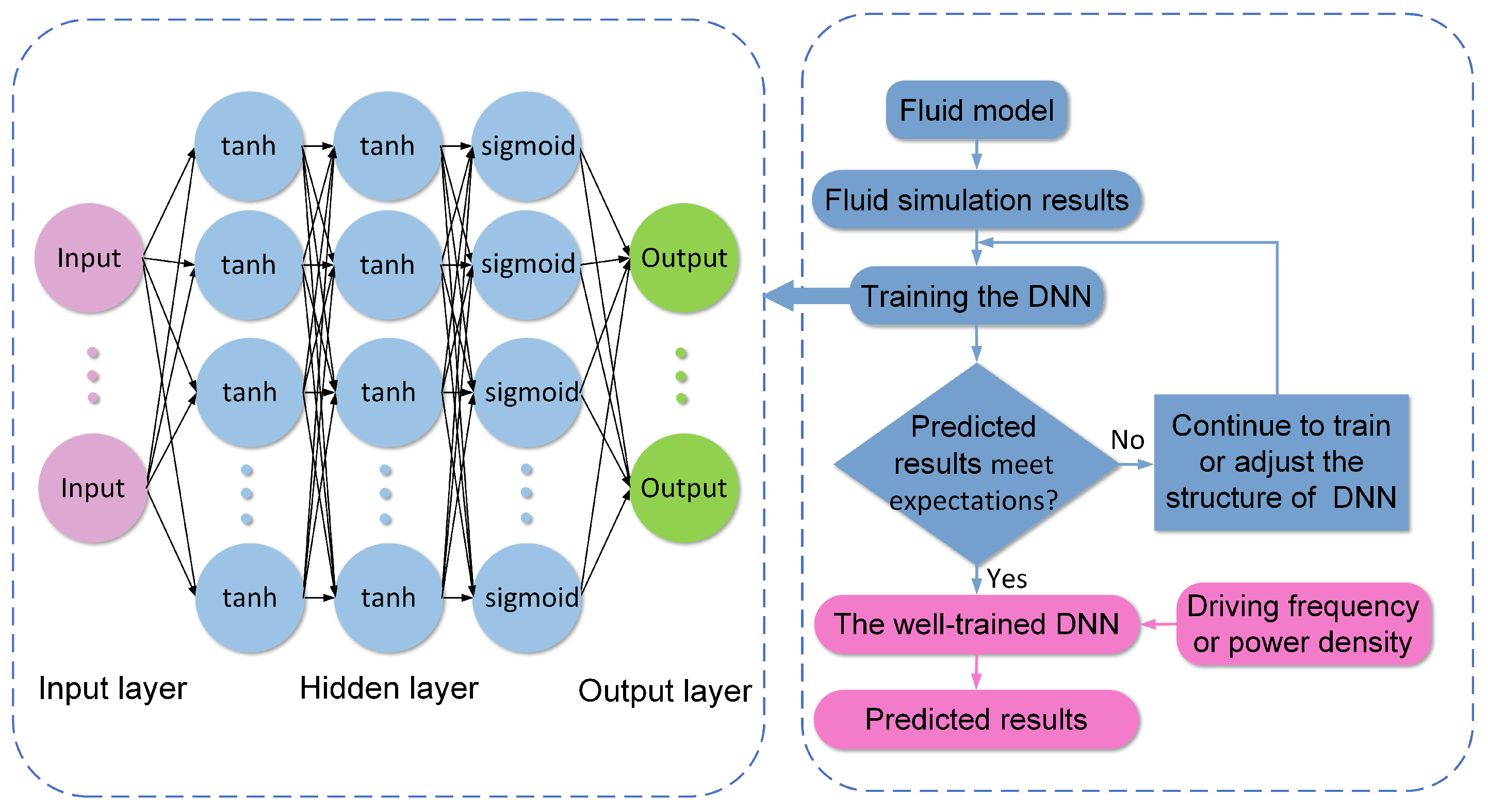
2.2. Description of DNN

In this section, a DNN is constructed to assist in modeling the RF ${\mathrm{CO}}_2$ discharges, as shown in Figure 1. Firstly, a training dataset for the DNN can be obtained from numerical simulations or experimental measurements, and in this study, the simulation data from the validated fluid model were used to train the DNN. Generally the training dataset is required to cover all the information in the sample space, i.e., the entire range of discharge parameters. The testing dataset is used to judge the prediction performance of the DNN model. If the prediction result of the DNN within the testing dataset meets the requirements (i.e., the average relative error between the prediction result and the simulation result is less than 0.5%), then it indicates that the DNN has good generalization performance within the given parameter range. The DNN constructed in this paper is a fully connected multilayer back-propagation neural network with one input layer, three hidden layers, and one output layer. From Figure 1, the circles in the schematic of the DNN denote the neurons that can accept the activations of the neurons from the previous layer as the input and perform a linear transformation, followed by an elementwise nonlinear transformation, and then, propagate the results to the next layer. Up to now, several studies have reported some experience in selecting the number and size of the hidden layers [51,52], but there are no rigorous rules for selecting these quantities. The appropriate network configuration is usually obtained by extensive experimentation. In general, more hidden layers and neurons are usually adopted to accurately predict the properties of complex systems, but an excessive number of hidden layers and neurons may lead to the overfitting of DNNs [53,54]. Based on the characteristics of RF ${\mathrm{CO}}_2$ discharges under Martian pressure, three hidden layers with 40 neurons per layer are adopted in the DNN constructed in Figure 1, and the tanh function and the sigmoid function are used as activation functions in the three hidden layer species in turn. The dimensions of the input layer and output layer determine the size of the input layer and output layer of the DNN. In this paper, the input of the DNN is the driving frequency and power density, and the output is the current–voltage characteristics, electric field, electron temperature, and product particle density. In addition, the selection of training data is related to the training efficiency and prediction performance of the DNN. If the amount of training data is small, it will reduce the training efficiency and lead to the prediction results of DNNs that do not meet the expectations. In contrast, using a large amount of training data may bring a huge computational load to the fluid simulation and DNN training.

In this work, 24 sets of simulation data obtained from the fluid model with a driving frequency between 12 and 75 MHz and 26 sets of simulation data with the power density between 35 and 85 W/cm² were used as the training data. For the discharge current and voltage, 2730 time points were sampled uniformly per set of simulated data. For the electric field, 300 space points in each set of the simulated dataset were sampled uniformly, and the same is true for each product particle density. The fluid simulation results for driving frequencies of 13.56, 27.12, 40.68, 54.24, and 67.80 MHz and power densities of 40, 50, 60, 70, and 80 W/cm² were selected as the testing dataset.

2.3. Validation of DNN

Before the prediction of more data, the validation of the DNN should be performed, by comparing the predicted results obtained from the DNN with the simulation results calculated by the fluid model. The predicted results of the DNN are in good agreement with the fluid simulation results within the testing dataset, and the MREs for various discharge characteristics are less than 0.5%. To illustrate the good accuracy and high efficiency of the DNN, a comparison of the predicted discharge characteristics and plasma chemistry of RF ${\mathrm{CO}}_2$ discharges at a frequency of 13.56 MHz and a power density of 60 W/cm² with the corresponding fluid simulation results is given. Figure 2 shows the predictions for the temporal evolutions of current density and voltage at a power density of 60 W/cm² and a driving frequency of 13.56 MHz, as well as the simulation results obtained from the fluid model. The solid and dashed lines in Figure 2 indicate the simulation and prediction results, respectively. It can be seen from the comparison in Figure 2 that the DNN yields very good predictions both in the current density and voltage domains, and the MREs for the current density and voltage are 0.18% and 0.42%, respectively.

Figure 3 displays the spatial profiles of the time-averaged positive charge density, negative charge density, and electric field predicted by the DNN, together with the corresponding profiles simulated by the fluid model. As shown in Figure 3, the DNN predictions agree well with the simulation results, even in the sheath regions, where the electric field varies sharply. The MREs of positive charge density, negative charge density, and electric field in this case are 0.14%, 0.16%, and 0.41%, respectively. The bell-shaped spatial profiles for positive and negative charges are given in Figure 3 with the accumulation in the central region between electrodes, indicating that most charged particles are trapped in the bulk plasma region in RF discharge. In addition, the density of positive charges near the electrodes is significantly higher than that of negative charges, leading to the formation of a space charge region accompanied by a stronger electric field.

Then, the DNN predictions for the spatial distributions of product particle density are also compared with the simulation results. Figure 4 shows the spatial distributions of the time-averaged density of the charged particles predicted by the DNN at a power density of 60 W/cm² and a driving frequency of 13.56 MHz with the comparison of the simulation results obtained from the fluid model. Good agreement can be observed in Figure 4, and the MREs of the electron density, ${\mathrm{CO}}_2^{+}$ density, ${\mathrm{O}}_2^{+}$ density, ${\mathrm{O}}^{-}$ density, and ${\mathrm{CO}}_3^{-}$ density were also measured, which are 0.05%, 0.16%, 0.47%, 0.64%, and 0.16%, respectively. As illustrated in Figure 4, the density of the electrons is the highest among all the negative charges, reaching $1.31\times {10}^{12}$ ${\mathrm{cm}}^{-3}$ in the bulk plasma region. The densities of the ${\mathrm{O}}^{-}$ and ${\mathrm{CO}}_3^{-}$ ions are an order of magnitude lower than that of electrons. The ${\mathrm{CO}}_2^{+}$ ions are the dominant positive charge with a maximum density of $1.26\times {10}^{12}$ ${\mathrm{cm}}^{-3}$, followed by the ${\mathrm{O}}_2^{+}$ ions with a maximum density of $4.73\times {10}^{11}$ ${\mathrm{cm}}^{-3}$.

The vibrationally excited ${\mathrm{CO}}_2$ is considered to play a key role in the splitting of ${\mathrm{CO}}_2$ under Martian pressure. Figure 5 plots the spatial distributions of the time-average vibrationally excited ${\mathrm{CO}}_2$ density predicted by the DNN, together with the simulation results obtained from the fluid model. As shown in Figure 5, the DNN prediction results agree well with the simulation results, and the MRE of the vibrationally excited ${\mathrm{CO}}_2$ is only 0.036%. From Figure 5, it is obvious that higher vibrational levels of ${\mathrm{CO}}_2$ possess a larger density. In RF ${\mathrm{CO}}_2$ discharges under Martian pressure, a large number of ${\mathrm{CO}}_2$ molecules at lower vibrational levels can gain vibrational energy through vibration–vibration (VV) relaxation and then be pumped to higher vibrational levels through the step-climbing mechanism along asymmetric stretching mode, leading to an increase in the density of higher vibrational levels. Neutral particles are the primary concerns of ISRU on Mars, so it is important to accurately predict the spatial distribution of neutral particles, such as CO, O, and ${\mathrm{O}}_2$.

More importantly, the high computational efficiency of the DNN needs to be emphasized. The conventional fluid simulations using the improved Scharfetter–Gummel (iSG) method [55] to solve multiple governing equations require at least 20,000 RF cycles of operation to ensure that the various properties of ${\mathrm{CO}}_2$ discharges achieve the dynamic steady state, which takes about 6 h (∼21,600 s). However, if the time to call the library functions is not considered, after about two hours of training, the DNN can yield the corresponding essential characteristics of RF ${\mathrm{CO}}_2$ discharge in about 0.01 s with very high accuracy. It can be said that the well-trained DNN improves the computational efficiency by a factor of about ${10}^6$ times with respect to the conventional fluid simulations of similar accuracy. In other words, the application of the DNN enables almost real-time prediction of various characteristics of RF ${\mathrm{CO}}_2$ discharge. Hence, the introduction of the DNN enables revealing the discharge characteristics and plasma chemistry in real time, although tens of species and hundreds of reactions are considered in CO₂ discharges; simultaneously, enough data can be predicted very efficiently by the DNN to more accurately describe the discharge evolution in RF CO₂ discharges.

3. Results and Discussion

Due to the high computational efficiency of the DNN, more simulation data can be calculated and the discharge characteristics can be predicted in detail in CO₂ discharges under Martian pressure at a given power density, which could allow discussing the effects of the driving frequency fairly on the RF discharges.

In this section, the well-trained DNN is applied to predict the discharge characteristics and plasma chemistry of RF ${\mathrm{CO}}_2$ discharges under Martian pressure for various driving frequencies at a given power density of 60 W/cm². Figure 6 shows the root-mean-squared (RMS) value of the current density and the RMS voltage as a function of the driving frequency at a fixed power density of 60 W/cm². When the driving frequency is increased from 12 to 75 MHz, the RMS current density is also increased from 58.5 to 114 $\mathrm{mA}/{\mathrm{cm}}^2$, almost two-fold growth, but at the same time, the RMS voltage is reduced from 317.5 V to 166.60 V, a decrease of about 1.91-times. The evolution of the current density and voltage at a given power density is consistent with the available experimental and simulation results [23,30,56], which further demonstrates the validation of the DNN constructed in the present study.

Figure 7 plots the predictions for the spatial distributions of the time-averaged electric fields driven by the five different frequencies. After good training, the DNN can obtain the spatial profile of the electric field at any driving frequency in about 0.01 s. As shown in Figure 7, the maximum value of the electric field appears in the sheath region, that is at the electrode surface. According to the predicted data, the maximum electric field decreases from 3.78 to 2.25 $\mathrm{kV}/\mathrm{cm}$, partly because of the reduction in the applied voltage, and the thickness of the sheath region reduces from 184 to 105 $\mathsf{\mu }\mathrm{m}$ with the growth of the driving frequency from 13.56 to 67.8 MHz when the power density is fixed at 60 W/cm². This indicates that an increase in the driving frequency can effectively decrease the sheath electric field and compress the sheath region.

Based on the prediction data, the predictions for the spatial profiles of the time-averaged electron density for various driving frequencies can be quickly obtained. From Figure 8, for a higher driving frequency, a larger electron density can be obtained with the maximum value located in the bulk plasma region. By altering the driving frequency from 13.56 to 67.8 MHz at a given power density of 60 W/cm², the maximum time-averaged electron density is also increased from $1.31\times {10}^{12}$ to $2.75\times {10}^{12}$ ${\mathrm{cm}}^{-3}$, almost 2.1-fold growth. The increase in the electron density can be attributed to the enhancement of electron trapping with increasing driving frequency [57]. Then, the effect of the driving frequency on the electron temperature is shown in Figure 9, which gives the spatial distributions of the time-averaged electron density predicted by the DNN for various driving frequencies. As shown in Figure 9, the maximum electron temperature is achieved in the sheath region due to the acceleration of the sheath fields, and this maximum value decreases with the increase in frequency. The electron temperature in the sheath region decreases mainly for the reduction of the sheath electric field.

In ${\mathrm{CO}}_2$ plasma, the vibrational energy in the vibrationally excited ${\mathrm{CO}}_2$ molecules can reduce the energy barrier of ${\mathrm{CO}}_2$ dissociation. The effects of the driving frequency on the behaviors of the asymmetric stretching mode of ${\mathrm{CO}}_2$ molecules are also described by the well-trained DNN. Figure 10 gives the spatial profiles of the time-averaged densities of the asymmetric stretching mode of ${\mathrm{CO}}_2$ molecules predicted by the DNN as a function of driving frequency at a given power density of 60 W/cm², where Figure 10a–h correspond to the spatial profiles of the time-averaged densities of ${\mathrm{CO}}_2{\mathrm{v}}_1$–${\mathrm{CO}}_2{\mathrm{v}}_8$, respectively. As shown in Figure 10, the well-trained DNN can give the profiles of the asymmetric stretching mode of ${\mathrm{CO}}_2$ molecules with various driving frequencies as a surface, instead of individual lines. It can be seen that the densities of the asymmetric stretching modes increase monotonically with the driving frequency. In fact, the behaviors of the asymmetric stretching modes can be attributed to the competition between the electron impact vibrational excitation, VV relaxation, and vibration–translation (VT) relaxation [45]. When the power density is fixed as a constant, as the driving frequency increases, the characteristic time of VT relaxation increases, while the characteristic time of vibrational excitation and VV relaxation decreases, which explains why the density of asymmetric stretching modes increases with the driving frequency. Furthermore, as shown in Figure 10, it can be observed that the peak density of lower vibrational levels is closer to the electrode surface. In fact, the electron impact vibrational excitation and VV relaxation are the dominant reactions for the generation of asymmetric stretching modes. A considerable fraction of the lower vibrational energy levels are generated by electron impact vibrational excitation due to their lower threshold energy of vibrational excitation. In the sheath region, the strong electric field accelerates the electrons, resulting in a more efficient vibrational excitation process. Therefore, the maximum density of lower vibrational levels appears in the sheath region.

Similarly, Figure 11 displays the prediction surfaces for the spatial distributions of the CO and ${\mathrm{O}}_2$ densities as a function of the driving frequency at a given power density of 60 W/cm². According to the predicted data shown in Figure 11a, with the increase in the driving frequency from 12 to 75 MHz, the maximum CO density obtained in the bulk region increases from $7.02\times {10}^{14}$ to $2.61\times {10}^{15}$ ${\mathrm{cm}}^{-3}$ by a factor of 3.72. In RF ${\mathrm{CO}}_2$ discharges under Martian pressure, the electron impact dissociation reaction ($\mathrm{e}+{\mathrm{CO}}_2\to \mathrm{e}+\mathrm{CO}+\mathrm{O}$) is the main pathway to generate CO. As the frequency increases, although the electron temperature decreases, the increase in the electron density and vibrationally excited ${\mathrm{CO}}_2$ density still enhances the electron impact dissociation reaction with the excited-state ${\mathrm{CO}}_2$. As a result, the density of CO increases with the driving frequency. The predictions for the spatial distributions of the ${\mathrm{O}}_2$ density as a function of the driving frequency are given in Figure 11b, showing a similar trend to the evolution of CO density in Figure 11a. When the driving frequency is 75 MHz, the maximum time-averaged density of ${\mathrm{O}}_2$ reaches $8.98\times {10}^{13}$ ${\mathrm{cm}}^{-3}$ at a given power density of 60 W/cm², nearly 2.05-times larger than that of $4.39\times {10}^{13}$ ${\mathrm{cm}}^{-3}$ at a driving frequency of 12 MHz. The ion reaction ($\mathrm{e}+{\mathrm{CO}}_2^{+}\to \mathrm{C}+{\mathrm{O}}_2$) is the dominant reaction for the formation of ${\mathrm{O}}_2$. From the discussion in Figure 8, it is clear that the densities of electrons and the ${\mathrm{CO}}_2^{+}$ ions in the discharge region rise with the driving frequency, which could improve the rate of the ion reaction ($\mathrm{e}+{\mathrm{CO}}_2^{+}\to \mathrm{C}+{\mathrm{O}}_2$), leading to a growth of the ${\mathrm{O}}_2$ density.

The well-trained DNN can give the behaviors of various species (such as charged species, neutral species, and excited species) formed in ${\mathrm{CO}}_2$ plasma at different driving frequencies as a surface instead of separate lines. Similar prediction surfaces can be achieved using the DNN for the electric field and electron temperature. In other words, for RF ${\mathrm{CO}}_2$ discharges driven at any frequency between 12 and 75 MHz, the DNN can obtain the corresponding discharge characteristics and plasma chemistry in 0.01 s with the same accuracy as the fluid simulation, which suggests that the essential characteristics of the ${\mathrm{CO}}_2$ conversion in RF discharge under Martian pressure could be given in real time as the driving frequency changes. Based on tens of training datasets calculated from the fluid model, the DNN can yield nearly infinite prediction results in a given parameter range after good training, which greatly expands the parameter-traversal range of RF ${\mathrm{CO}}_2$ discharge.

Figure 12 provides the profiles of the ${\mathrm{CO}}_2$ conversion versus the driving frequency at a given power density of 60 W/cm². A slight increase in ${\mathrm{CO}}_2$ conversion with increasing driving frequency can be observed in Figure 12. According to the prediction results, the ${\mathrm{CO}}_2$ conversion increases from 24.2% to 26.8% as the frequency changes from 12 MHz to 75 MHz. As the driving frequency increases, a considerable fraction of the energy is transferred from the electrons to the asymmetric stretching modes, increasing the density of the asymmetric stretching modes. The vibrational energy in the asymmetric stretching modes can lower the energy barrier of ${\mathrm{CO}}_2$ decomposition; thus, the increase in the driving frequency enhances the rates of the electron impact reactions with vibrationally excited ${\mathrm{CO}}_2$, leading to an improvement in ${\mathrm{CO}}_2$ conversion.

The input power has a significant impact on the ${\mathrm{CO}}_2$ conversion in RF discharges under Martian pressure. Therefore, the well-trained DNN was employed to predict the effects of the input power on the discharge characteristics and plasma chemistry of RF ${\mathrm{CO}}_2$ discharges from the perspective of the electric field, particle density, and ${\mathrm{CO}}_2$ conversion.

The predicted spatial distributions of the time-averaged electric field are given in Figure 13 using the well-trained DNN for various power densities at a driving frequency of 13.56 MHz. The electric field in the sheath region is significantly enhanced as more power is coupled to the RF plasmas. With the growth of the power density from 40 to 60 to 80 W/cm², the maximum electric field increases monotonically from 3.15 to 3.79 to 4.28 kV/cm from the predicted data. In addition, the variation in the thickness of the sheath region can be neglected as the input power density varies. The strong sheath electric field is able to accelerate the electrons and improve the electron temperature.

To gain insight into the variation of the neutral particles formed in ${\mathrm{CO}}_2$ plasma as the power density varies, the spatial distributions of the time-averaged CO density and ${\mathrm{O}}_2$ density as a function of the power density are predicted by the DNN in almost real time. From Figure 14a, the maximum CO density is $1.57\times {10}^{14}$ ${\mathrm{cm}}^{-3}$ when the power density is 35 W/cm². As the power density is improved to 85 W/cm², the peak CO density reaches $1.52\times {10}^{15}$ ${\mathrm{cm}}^{-3}$. The production of CO is mainly through electron impact dissociation processes. From the above analysis, more energetic electrons are produced with the growth of the power density, enhancing the rate of the dissociation process. As a result, a higher CO density can be achieved as the power density grows. Meanwhile, a similar evolutionary trend of ${\mathrm{O}}_2$ density can be observed in Figure 14b. When the power density increases from 35 to 85 W/cm², the maximum time-averaged ${\mathrm{O}}_2$ density rises from $2.84\times {10}^{13}$ to $6.67\times {10}^{13}$ ${\mathrm{cm}}^{-3}$ based on the well-trained DNN. The primary reaction of producing ${\mathrm{O}}_2$ is the ion reaction ($\mathrm{e}+{\mathrm{CO}}_2^{+}\to \mathrm{C}+{\mathrm{O}}_2$). Since the electron density and ${\mathrm{CO}}_2^{+}$ density improve as the power density increases, then an increase in ${\mathrm{O}}_2$ density can be observed in Figure 14b.

The effect of the power density on ${\mathrm{CO}}_2$ conversion is also described by using the well-trained DNN in this paper. Figure 15 gives the ${\mathrm{CO}}_2$ conversion as a function of the power density at a given driving frequency of 13.56 MHz. An improvement of ${\mathrm{CO}}_2$ conversion can be observed with the power density, which can also be revealed directly by the fluid model. According to Figure 15, when the power density increases from 35 to 85 W/cm², the ${\mathrm{CO}}_2$ conversion only rises from 23.2% to 25.1%, which indicates that increasing the input power density at a given RF frequency can improve the ${\mathrm{CO}}_2$ conversion in RF discharges, but not significantly. Although more power is coupled into the discharge system, the key reactions corresponding to the conversion do not become more effective, while the gas heating is enhanced in RF discharge.

4. Conclusions

In this study, a DNN is constructed with three hidden layers instead of the time-consuming fluid model to describe the ${\mathrm{CO}}_2$ conversion in RF discharges at a given power density under Martian pressure involving tens of species and hundreds of reactions. A DNN that was well trained on the simulation data or experimental measurements was employed to describe the discharge characteristics and plasma chemistry of RF ${\mathrm{CO}}_2$ discharges for various driving frequencies and power densities. The predicted results showed a good agreement with the fluid simulation results, and the MREs of various characteristics were less than 0.5%. It should be note that the qualified experimental data can also be applied to work as the training data; actually, the training dataset of a DNN only requires data of good quality and sufficient quantity, without concern regarding the source of the data. Usually, the fluid simulations solving the governing equations require nearly 20,000 s to obtain stable results on a given computational platform; however, after nearly two hours of training, the DNN only needed about 0.01 s to yield the key characteristics of the RF ${\mathrm{CO}}_2$ discharge, such as the current–voltage characteristics, the electric field profiles, and the distribution of the particle densities. Compared to the traditional fluid model, the computational efficiency of the DNN was improved by about ${10}^6$-times, which indicates that the DNN could achieve almost real-time calculation of the ${\mathrm{CO}}_2$ conversion in RF discharges with tens of species and hundreds of reactions. Due to the high computational efficiency, the DNN can provide a much larger amount of data than the traditional fluid model to enhance the simulation results, to show the spatial distributions of plasma species as a surface rather than as individual lines for various driving frequencies and input power densities, which vividly illustrate the evolution of the data and reveal more details about the underpinning physics. In addition, the DNN was applied to investigate the effects of the driving frequency and input power density on the ${\mathrm{CO}}_2$ conversion in RF discharges. The predicted results also showed that, by increasing the driving frequency at a constant power density, an increase in the density of charged particles, neutral particles, and vibrationally excited ${\mathrm{CO}}_2$ molecules can be observed; meanwhile, the ${\mathrm{CO}}_2$ conversion also increases with the driving frequency. In addition, a slight improvement in ${\mathrm{CO}}_2$ conversion was also observed as more power was coupled into the RF plasma. The study suggests that the DNN has an excellent ability to describe the discharge characteristics and plasma chemistry of RF ${\mathrm{CO}}_2$ discharges with tens of species and hundreds of reactions. Data-driven models, such as DNNs, offer a promising approach to investigate plasma-based ${\mathrm{CO}}_2$ conversion for various applications, which can be extended to more complex plasma modeling in future work.

References

1. Meyen, F.E.; Hecht, M.H.; Hoffman, J.A.; Team, M. Thermodynamic model of Mars oxygen ISRU experiment (MOXIE). Acta Astronaut. 2016, 129, 82–87. [Google Scholar] [CrossRef]
2. Starr, S.O.; Muscatello, A.C. Mars in situ resource utilization: A review. Planet. Space Sci. 2020, 182, 104824. [Google Scholar] [CrossRef]
3. Chen, H.; du Jonchay, T.S.; Hou, L.; Ho, K. Integrated in-situ resource utilization system design and logistics for Mars exploration. Acta Astronaut. 2020, 170, 80–92. [Google Scholar] [CrossRef]
4. Hoffman, J.A.; Hecht, M.H.; Rapp, D.; Hartvigsen, J.J.; SooHoo, J.G.; Aboobaker, A.M.; McClean, J.B.; Liu, A.M.; Hinterman, E.D.; Nasr, M. Mars Oxygen ISRU Experiment (MOXIE)—Preparing for human Mars exploration. Sci. Adv. 2022, 8, eabp8636. [Google Scholar] [CrossRef] [PubMed]
5. Hartvigsen, J.; Elangovan, S.; Elwell, J.; Larsen, D. Oxygen production from Mars atmosphere carbon dioxide using solid oxide electrolysis. ECS Trans. 2017, 78, 2953. [Google Scholar] [CrossRef]
6. Gupta, T.T.; Ayan, H. Application of non-thermal plasma on biofilm: A review. Appl. Sci. 2019, 9, 3548. [Google Scholar] [CrossRef]
7. Hati, S.; Patel, M.; Yadav, D. Food bioprocessing by non-thermal plasma technology. Curr. Opin. Food Sci. 2018, 19, 85–91. [Google Scholar] [CrossRef]
8. Li, S.; Dang, X.; Yu, X.; Abbas, G.; Zhang, Q.; Cao, L. The application of dielectric barrier discharge non-thermal plasma in VOCs abatement: A review. Chem. Eng. J. 2020, 388, 124275. [Google Scholar] [CrossRef]
9. Guerra, V.; Silva, T.; Pinhão, N.; Guaitella, O.; Guerra-Garcia, C.; Peeters, F.J.J.; Tsampas, M.N.; van de Sanden, M.C.M. Plasmas for in situ resource utilization on Mars: Fuels, life support, and agriculture. J. Appl. Phys. 2023, 51, 49–59. [Google Scholar] [CrossRef]
10. George, A.; Shen, B.; Craven, M.; Wang, Y.; Kang, D.; Wu, C.; Tu, X. A Review of Non-Thermal Plasma Technology: A novel solution for CO2 conversion and utilization. Renew. Sustain. Energy Rev. 2021, 135, 109702. [Google Scholar] [CrossRef]
11. Guerra, V.; Silva, T.; Ogloblina, P.; Grofulović, M.; Terraz, L.; da Silva, M.L.; Pintassilgo, C.D.; Alves, L.L.; Guaitella, O. The case for in situ resource utilisation for oxygen production on Mars by non-equilibrium plasmas. Plasma Sources Sci. Technol. 2017, 26, 11LT01. [Google Scholar] [CrossRef]
12. Ogloblina, P.; Morillo-Candas, A.S.; Silva, A.F.; Silva, T.; Tejero-del Caz, A.; Alves, L.L.; Guaitella, O.; Guerra, V. Mars in situ oxygen and propellant production by non-equilibrium plasmas. Plasma Sources Sci. Technol. 2021, 30, 065005. [Google Scholar] [CrossRef]
13. Yu, Q.Q.; Kong, M.; Liu, T.; Fei, J.H.; Zheng, X.M. Characteristics of the decomposition of CO2 in a dielectric packed-bed plasma reactor. Plasma Chem. Plasma Process. 2012, 32, 153–163. [Google Scholar] [CrossRef]
14. Aerts, R.; Somers, W.; Bogaerts, A. Carbon dioxide splitting in a dielectric barrier discharge plasma: A combined experimental and computational study. ChemSusChem 2015, 8, 702–716. [Google Scholar] [CrossRef] [PubMed]
15. Zhang, H.; Li, L.; Li, X.D.; Wang, W.Z.; Yan, J.H.; Tu, X. Warm plasma activation of CO2 in a rotating gliding arc discharge reactor. J. CO2 Util. 2018, 27, 472–479. [Google Scholar] [CrossRef]
16. Nunnally, T.; Gutsol, K.; Rabinovich, A.; Fridman, A.; Gutsol, A.; Kemoun, A. Dissociation of CO2 in a low current gliding arc plasmatron. J. Phys. Appl. Phys. 2011, 44, 274009. [Google Scholar] [CrossRef]
17. Ong, M.Y.; Nomanbhay, S.; Kusumo, F.; Show, P.L. Application of microwave plasma technology to convert carbon dioxide (CO2) into high value products: A review. J. Clean. Prod. 2022, 336, 130447. [Google Scholar] [CrossRef]
18. Chen, G.; Britun, N.; Godfroid, T.; Georgieva, V.; Snyders, R.; Delplancke-Ogletree, M.P. An overview of CO2 conversion in a microwave discharge: The role of plasma-catalysis. J. Phys. Appl. Phys. 2017, 50, 084001. [Google Scholar] [CrossRef]
19. Spencer, L.F.; Gallimore, A.D. Efficiency of CO2 dissociation in a radio-frequency discharge. Plasma Chem. Plasma Process. 2011, 31, 79–89. [Google Scholar] [CrossRef]
20. Stanković, V.V.; Ristić, M.M.; Vojnović, M.M.; Aoneas, M.M.; Poparić, G.B. Ionization and Electronic State Excitation of CO2 in Radio-frequency Electric Field. Plasma Chem. Plasma Process. 2020, 40, 1621–1637. [Google Scholar] [CrossRef]
21. Huang, Q.; Zhang, D.; Wang, D.; Liu, K.; Kleyn, A.W. Carbon dioxide dissociation in non-thermal radiofrequency and microwave plasma. J. Phys. Appl. Phys. 2017, 50, 294001. [Google Scholar] [CrossRef]
22. Snoeckx, R.; Bogaerts, A. Plasma technology–a novel solution for CO2 conversion? Chem. Soc. Rev. 2017, 46, 5805–5863. [Google Scholar] [CrossRef] [PubMed]
23. Zhang, Y.T.; Cui, S.Y. Frequency effects on the electron density and α-γ mode transition in atmospheric radio frequency discharges. Phys. Plasmas 2011, 18, 083509. [Google Scholar] [CrossRef]
24. Zhang, Y.T.; He, J. Frequency effects on the production of reactive oxygen species in atmospheric radio frequency helium-oxygen discharges. Phys. Plasmas 2013, 20, 013502. [Google Scholar] [CrossRef]
25. Aerts, R.; Martens, T.; Bogaerts, A. Influence of vibrational states on CO2 splitting by dielectric barrier discharges. J. Phys. Chem. 2012, 116, 23257–23273. [Google Scholar] [CrossRef]
26. Kozák, T.; Bogaerts, A. Splitting of CO2 by vibrational excitation in non-equilibrium plasmas: A reaction kinetics model. Plasma Sources Sci. Technol. 2014, 23, 045004. [Google Scholar] [CrossRef]
27. Ponduri, S.; Becker, M.; Welzel, S.; Van De Sanden, M.; Loffhagen, D.; Engeln, R. Fluid modelling of CO2 dissociation in a dielectric barrier discharge. J. Appl. Phys. 2016, 119, 093301. [Google Scholar] [CrossRef]
28. Fu, Q.; Wang, Y.; Chang, Z. Study on the conversion mechanism of CO2 to O2 in pulse voltage dielectric barrier discharge at Martian pressure. J. CO2 Util. 2023, 70, 102430. [Google Scholar] [CrossRef]
29. Wang, X.C.; Zhang, T.H.; Sun, Y.; Wu, Z.C.; Zhang, Y.T. Numerical study on discharge characteristics and plasma chemistry in atmospheric CO2 discharges driven by pulsed voltages. Phys. Plasmas 2022, 29, 023505. [Google Scholar] [CrossRef]
30. Amanatides, E.; Mataras, D. Frequency variation under constant power conditions in hydrogen radio frequency discharges. J. Appl. Phys. 2001, 89, 1556–1566. [Google Scholar] [CrossRef]
31. Zhang, Y.T.; Li, Q.Q.; Lou, J.; Li, Q.M. The characteristics of atmospheric radio frequency discharges with frequency increasing at a constant power density. Appl. Phys. Lett. 2010, 97, 141504. [Google Scholar] [CrossRef]
32. Anirudh, R.; Archibald, R.; Asif, M.S.; Becker, M.M.; Benkadda, S.; Bremer, P.T.; Budé, R.H.; Chang, C.S.; Chen, L.; Churchill, R.; et al. 2022 review of data-driven plasma science. IEEE Trans. Plasma Sci. 2023, 51, 1750–1838. [Google Scholar] [CrossRef]
33. He, M.; Bai, R.; Tan, S.; Liu, D.; Zhang, Y. Data-driven plasma science: A new perspective on modeling, diagnostics, and applications through machine learning. Plasma Process. Polym. 2024, e2400020. [Google Scholar] [CrossRef]
34. Hansen, K.; Biegler, F.; Ramakrishnan, R.; Pronobis, W.; Von Lilienfeld, O.A.; Muller, K.R.; Tkatchenko, A. Machine learning predictions of molecular properties: Accurate many-body potentials and nonlocality in chemical space. J. Phys. Chem. Lett. 2015, 6, 2326–2331. [Google Scholar] [CrossRef] [PubMed]
35. Sturm, I.; Lapuschkin, S.; Samek, W.; Müller, K.R. Interpretable deep neural networks for single-trial EEG classification. J. Neurosci. Methods 2016, 274, 141–145. [Google Scholar] [CrossRef] [PubMed]
36. Schütt, K.T.; Arbabzadah, F.; Chmiela, S.; Müller, K.R.; Tkatchenko, A. Quantum-chemical insights from deep tensor neural networks. Nat. Commun. 2017, 8, 13890. [Google Scholar] [CrossRef] [PubMed]
37. Garola, A.R.; Cavazzana, R.; Gobbin, M.; Delogu, R.S.; Manduchi, G.; Taliercio, C.; Luchetta, A. Diagnostic data integration using deep neural networks for real-time plasma analysis. IEEE Trans. Nucl. Sci. 2021, 68, 2165–2172. [Google Scholar] [CrossRef]
38. Liu, H.; Yang, M.; Liu, Y.; Geng, J.; Tang, J. A Deep-Learning-Based Method for Diagnosing Time-Varying Plasma Adopting Microwaves. IEEE Trans. Plasma Sci. 2021, 49, 1406–1413. [Google Scholar] [CrossRef]
39. Wang, X.C.; Zhang, Y.T. Modeling of discharge characteristics and plasma chemistry in atmospheric CO2 pulsed plasmas employing deep neural network. J. Appl. Phys. 2023, 133. [Google Scholar] [CrossRef]
40. Zhang, Y.T.; Gao, S.H.; Ai, F. Efficient numerical simulation of atmospheric pulsed discharges by introducing deep learning. Front. Phys. 2023, 11, 1125548. [Google Scholar] [CrossRef]
41. Nazari, R.R.; Hajizadeh, K. Modeling the performance of cold plasma in CO2 splitting using artificial neural networks. AIP Adv. 2022, 12, 085018. [Google Scholar] [CrossRef]
42. Karniadakis, G.E.; Kevrekidis, I.G.; Lu, L.; Perdikaris, P.; Wang, S.; Yang, L. Physics-informed machine learning. Nat. Rev. Phys. 2021, 3, 422–440. [Google Scholar] [CrossRef]
43. Wahbah, M.; Mohandes, B.; EL-Fouly, T.H.; El Moursi, M.S. Unbiased cross-validation kernel density estimation for wind and PV probabilistic modelling. Energy Convers. Manag. 2022, 266, 115811. [Google Scholar] [CrossRef]
44. Wang, X.C.; Bai, J.X.; Zhang, T.H.; Sun, Y.; Zhang, Y.T. Comprehensive study on plasma chemistry and products in CO2 pulsed discharges under Martian pressure. Vacuum 2022, 203, 111200. [Google Scholar] [CrossRef]
45. Wang, X.C.; Gao, S.H.; Zhang, Y.T. Frequency Effects on the Vibrational States and Conversion of CO2 in Radio Frequency Discharges Under Martian Pressure. IEEE Trans. Plasma Sci. 2022, 51, 49–59. [Google Scholar] [CrossRef]
46. Simeni, M.S.; Zheng, Y.; Barnat, E.V.; Bruggeman, P.J. Townsend to glow discharge transition for a nanosecond pulse plasma in helium: Space charge formation and resulting electric field dynamics. Plasma Sources Sci. Technol. 2021, 30, 055004. [Google Scholar] [CrossRef]
47. Deconinck, T.; Mahadevan, S.; Raja, L.L. Discretization of the Joule heating term for plasma discharge fluid models in unstructured meshes. J. Comput. Phys. 2009, 228, 4435–4443. [Google Scholar] [CrossRef]
48. Yuan, X.; Raja, L.L. Computational study of capacitively coupled high-pressure glow discharges in helium. IEEE Trans. Plasma Sci. 2003, 31, 495–503. [Google Scholar] [CrossRef]
49. Wang, X.C.; Bai, J.X.; Zhang, T.H.; Sun, Y.; Zhang, Y.T. Comprehensive study on discharge characteristics in pulsed dielectric barrier discharges with atmospheric He and CO2. Phys. Plasmas 2022, 29, 083503. [Google Scholar] [CrossRef]
50. Wang, C.; Fu, Q.; Chang, Z.; Zhang, G. Investigation on the products distribution, reaction pathway, and discharge mechanism of low-pressure CO2 discharge by employing a 1D simulation model. Plasma Process. Polym. 2021, 18, 2000228. [Google Scholar] [CrossRef]
51. Bengio, Y. Practical recommendations for gradient-based training of deep architectures. In Neural Networks: Tricks of the Trade, 2nd ed.; Springer: Berlin/Heidelberg, Germany, 2012; pp. 437–478. [Google Scholar]
52. Karsoliya, S. Approximating number of hidden layer neurons in multiple hidden layer BPNN architecture. Int. J. Eng. Trends Technol. 2012, 3, 714–717. [Google Scholar]
53. Srivastava, N.; Hinton, G.; Krizhevsky, A.; Sutskever, I.; Salakhutdinov, R. Dropout: A simple way to prevent neural networks from overfitting. J. Mach. Learn. Res. 2014, 15, 1929–1958. [Google Scholar]
54. Sharma, S.; Sharma, S.; Athaiya, A. Activation functions in neural networks. Towards Data Sci. 2017, 6, 310–316. [Google Scholar] [CrossRef]
55. Kulikovsky, A.A. A more accurate Scharfetter-Gummel algorithm of electron transport for semiconductor and gas discharge simulation. J. Comput. Phys. 1995, 119, 149–155. [Google Scholar] [CrossRef]
56. Walsh, J.L.; Iza, F.; Kong, M.G. Atmospheric glow discharges from the high-frequency to very high-frequency bands. Appl. Phys. Lett. 2008, 93, 251502. [Google Scholar] [CrossRef]
57. Liu, D.W.; Shi, J.J.; Kong, M.G. Electron trapping in radio-frequency atmospheric-pressure glow discharges. Appl. Phys. Lett. 2007, 90, 041502. [Google Scholar] [CrossRef]
Figure 1. Schematic diagram of DNN-assisted RF CO 2 discharge modeling method.
Applsci 14 06855 g001
Figure 2. Temporal evolutions of current density and voltage predicted by the DNN in RF CO 2 discharge with a comparison of the results obtained from the fluid simulation. Red dotted line: the predicted current density; green dotted line: the predicted voltage.
Applsci 14 06855 g002
Figure 3. Spatial distributions of time-averaged positive charge density, negative charge density, and electric field predicted by the DNN with a comparison of the results obtained from the fluid simulation.
Applsci 14 06855 g003
Figure 4. Spatial distributions of time-average charged particle density predicted by the DNN with a comparison of the results obtained from the fluid simulation.
Applsci 14 06855 g004
Figure 5. Spatial distributions of time-average vibrationally excited CO 2 density predicted by the DNN with a comparison of the results obtained from the fluid simulation.
Applsci 14 06855 g005
Figure 6. RMS current density and RMS voltage predicted by the DNN as a function of the driving frequency at a given power density of 60 W/cm2.
Applsci 14 06855 g006
Figure 7. Spatial distributions of the time-averaged electric field predicted by the DNN for various driving frequencies at a given power density of 60 W/cm2.
Applsci 14 06855 g007
Figure 8. Spatial distributions of the time-averaged electron density predicted by the DNN for various driving frequencies at a given power density of 60 W/cm2.
Applsci 14 06855 g008
Figure 9. Spatial distributions of the time-averaged electron temperature predicted by the DNN for various driving frequencies at a given power density of 60 W/cm2.
Applsci 14 06855 g009
Figure 10. Spatial distributions of the time-averaged densities of the asymmetric stretching mode of CO 2 molecules ((a) CO 2 v 1 , (b) CO 2 v 2 , (c) CO 2 v 3 , (d) CO 2 v 4 , (e) CO 2 v 5 , (f) CO 2 v 6 , (g) CO 2 v 7 , and (h) CO 2 v 8 ) predicted by the DNN as a function of the driving frequency at a given power density of 60 W/cm2.
Applsci 14 06855 g010
Figure 11. Spatial distributions of the time-averaged (a) CO density and (b) O 2 density predicted by the DNN as a function of the driving frequency at a given power density of 60 W/cm2.
Applsci 14 06855 g011
Figure 12. The CO 2 conversion predicted by the DNN as a function of the driving frequency at a given power density of 60 W/cm2.
Applsci 14 06855 g012
Figure 13. Spatial distributions of the time-averaged electric field predicted by the DNN for various power densities at a driving frequency of 13.56 MHz.
Applsci 14 06855 g013
Figure 14. Spatial distributions of the time-averaged (a) CO density and (b) O 2 density predicted by the DNN as a function of the power density at a given driving frequency of 13.56 MHz.
Applsci 14 06855 g014
Figure 15. The CO 2 conversion predicted by the DNN as a function of the power density at a given driving frequency of 13.56 MHz.
Applsci 14 06855 g015
Disclaimer/Publisher’s Note: The statements, opinions and data contained in all publications are solely those of the individual author(s) and contributor(s) and not of MDPI and/or the editor(s). MDPI and/or the editor(s) disclaim responsibility for any injury to people or property resulting from any ideas, methods, instructions or products referred to in the content.