A Genetic Programming Approach to Radiomic-Based Feature Construction for Survival Prediction in Non-Small Cell Lung Cancer

Abstract

Machine learning (ML) is commonly used to develop survival-predictive radiomic models in non-small cell lung cancer (NSCLC) patients, which helps assist treatment decision making. Radiomic features derived from computer tomography (CT) lung images aim to capture quantitative tumor characteristics. However, these features are determined by humans, which poses a risk of including irrelevant or redundant variables, thus reducing the model’s generalization. To address this issue, we propose using genetic programming (GP) to automatically construct new features with higher discriminant power than the original radiomic features. To achieve this goal, we introduce a fitness function that measures the classification performance ratio of output to input. The constructed features are then input for various classifiers to predict the two-year survival of NSCLC patients from two public CT datasets. Our approach is compared against two popular feature selection methods in radiomics to choose relevant radiomic features, and two GP-based feature construction methods whose fitness functions are based on measuring the constructed features’ quality. The experimental results show that survival prediction models trained on GP-based constructed features outperform feature selection methods. Also, maximizing the classification performance gain output-to-input ratio produces features with higher discriminative power than only maximizing the classification accuracy from constructed features. Furthermore, a survival analysis demonstrated statistically significant differences between survival and non-survival groups in the Kaplan–Meier curves. Therefore, the proposed approach can be used as a complementary method for oncologists in determining the clinical management of NSCLC patients.

1. Introduction

Lung cancer is the leading cause of mortality by malignant neoplasms worldwide, with an estimated 1.8 million deaths in 2020 [1]. In particular, non-small cell lung cancer (NSCLC) accounts for about 85% of all lung cancer patients. Computer tomography (CT) is the imaging modality adopted for lung cancer screening (in addition to low-dose CT) and lung cancer diagnosis. Despite the various diagnostic tools and novel treatments, the five-year survival rate for NSCLC is about 22%.

Accurate survival prediction following a cancer diagnosis is essential to guide treatment decision making [2]. In this context, machine learning (ML)-based systems could improve patients’ outcomes by assisting clinicians with accurate survival analysis, personalized treatment planning, and prognosis [3]. An ML-based diagnostic system traditionally comprises region of interest (ROI) detection or segmentation, feature extraction, and classification [4,5].

Feature extraction is crucial because the quantitative features extracted from lung images should be relevant and useful for developing applicable classification models. A widely used technique for NSCLC characterization is radiomics, which extracts high-throughput quantitative information from CT lung images [6]. Radiomic features comprise morphological, volumetric, histogram-based, and texture parameters that characterize the phenotypic representation of tumors [7]. They also serve as image biomarkers to assess tumor heterogeneity and predict clinical outcomes [8].

Conventional ML radiomic pipelines, composed of feature extraction, reduction, and classification techniques, have been employed in the literature to predict NSCLC survival. The first thorough evaluation of the ML radiomic pipeline was conducted by Parmar et al. [9], who investigated fourteen feature selection methods and twelve classification methods to predict NSCLC survival. They found that the Wilcoxon test-based feature selection method and the random forest classifier had the highest prognostic performance, with high stability against data perturbation. In another work, Zhang et al. [10] studied the effectiveness of merging five unsupervised feature reduction techniques and eight different classifiers utilizing CT radiomic features from an NSCLC dataset with three clinical outcomes: recurrence, death, and recurrence-free survival. They concluded that factors such as data endpoints, feature selection techniques, and classifiers significantly affect model accuracy, and thus, they should be carefully investigated when performing a radiomic analysis. More recently, Braghetto et al. [11] tested different ML pipelines for building radiomic models from CT images of NSCLC patients, reporting that the best combination was achieved by the ANOVA feature selection method with a random forest classifier. Additionally, other researchers have delved into diverse ML pipelines and algorithms to enhance prediction models based on CT radiomic features [12,13,14].

On the other hand, deep learning (DL) models have achieved remarkable performance in image classification tasks in recent years because of their automatic feature learning capability with different abstraction levels. Therefore, extracting deep features from convolutional neural networks (CNNs) is considered a primary alternative and valuable method to compute image-based parameters that could increase the classification power [15]. They have been used to predict survival in NSCLC patients on CT images [11,16] and can be combined with the traditional radiomic approach [17].

A disadvantage of radiomic features is the reliance on a human expert to define the set of features, risking missing relevant variables due to ignorance or failure to understand some complex, hidden, or non-intuitive phenomena [18]. This problem has been addressed using DL models; however, a well-known drawback is overfitting, mainly when using small-sized datasets, due to the high number of trainable parameters. This issue is because the more learnable parameters, the higher the possibility that activation patterns specific to examples in the training set will happen [15]. This limitation should be considered in NSCLC survival prediction, where collecting many annotated cases is challenging.

To address the above limitations, we propose enhancing radiomic features by automatically creating new ones with greater discriminant power. The created features can then be used in a traditional ML-based survival prediction system, where the prediction models are less complex than DL models and simpler to learn. We devised a feature construction approach based on genetic programming (GP) since it has proved versatile and effective in different cancer applications [19,20,21,22,23,24] and the design of radiomics systems [25], and its application to NSCLC survival prediction is novel.

GP is an evolutionary computation technique that uses Darwinian principles of reproduction and survival of the fittest to evolve a population of computer programs or mathematical expressions codified in syntactic tree representations [26]. GP-based feature construction approaches usually adopt a multi-tree representation to create a new multi-dimensional feature space, where each tree constructs a single feature [27]. Moreover, feature construction can be addressed by wrapper and filter approaches. The former measures the quality of the constructed features using classification performance, while the latter measures the statistical dependency of constructed features and the target variable.

Wrapper GP-based feature construction approaches typically use a fitness function that assesses the classification performance of the constructed features at the trees’ outputs [19,20,28,29]. These methods assume that the constructed features should outperform the original ones at the trees’ inputs. However, such an assumption is not guaranteed, and the constructed features may underperform the original ones.

Our previous research involved preliminary experiments with GP-based radiomic features to improve survival prediction in NSCLC compared to the traditional ML procedure [30]. In the current research, we have extended the previous work by proposing a new fitness function that measures the classification performance ratio of output to input to evaluate the impact of increasing both the trees’ depth and the number of trees (i.e., constructed features) using a multi-tree representation. This fitness function ensures that the constructed features improve upon the original radiomic features to address the wrapper approach’s limitations. Moreover, considering six classification methods, the proposed GP-based feature construction approach is evaluated on LUNG1 and LUNG2 public datasets [31,32]. Both contain NSCLC patients’ CT images and survival data and have been extensively used to develop ML and DL models [11]. Therefore, using the same datasets allows for a fair comparison with previous studies to predict the same clinical outcome.

It is worth remarking that clinical models tested on the LUNG1 dataset can achieve AUC values close to chance; neither radiomics nor DL models could provide high performances, achieving AUC values in the range of 0.61–0.67 [9,11,13,33]. Starting from these previous works, we aim to explore whether a GP-based approach can improve the accuracy of survival prediction in NSCLC by creating new discriminant features from radiomic ones. The goal is to increase the survival prediction performance in NSCLC patients, which could be used as a support for oncologists to determine the clinical prognosis of patients.

2. Materials and Methods

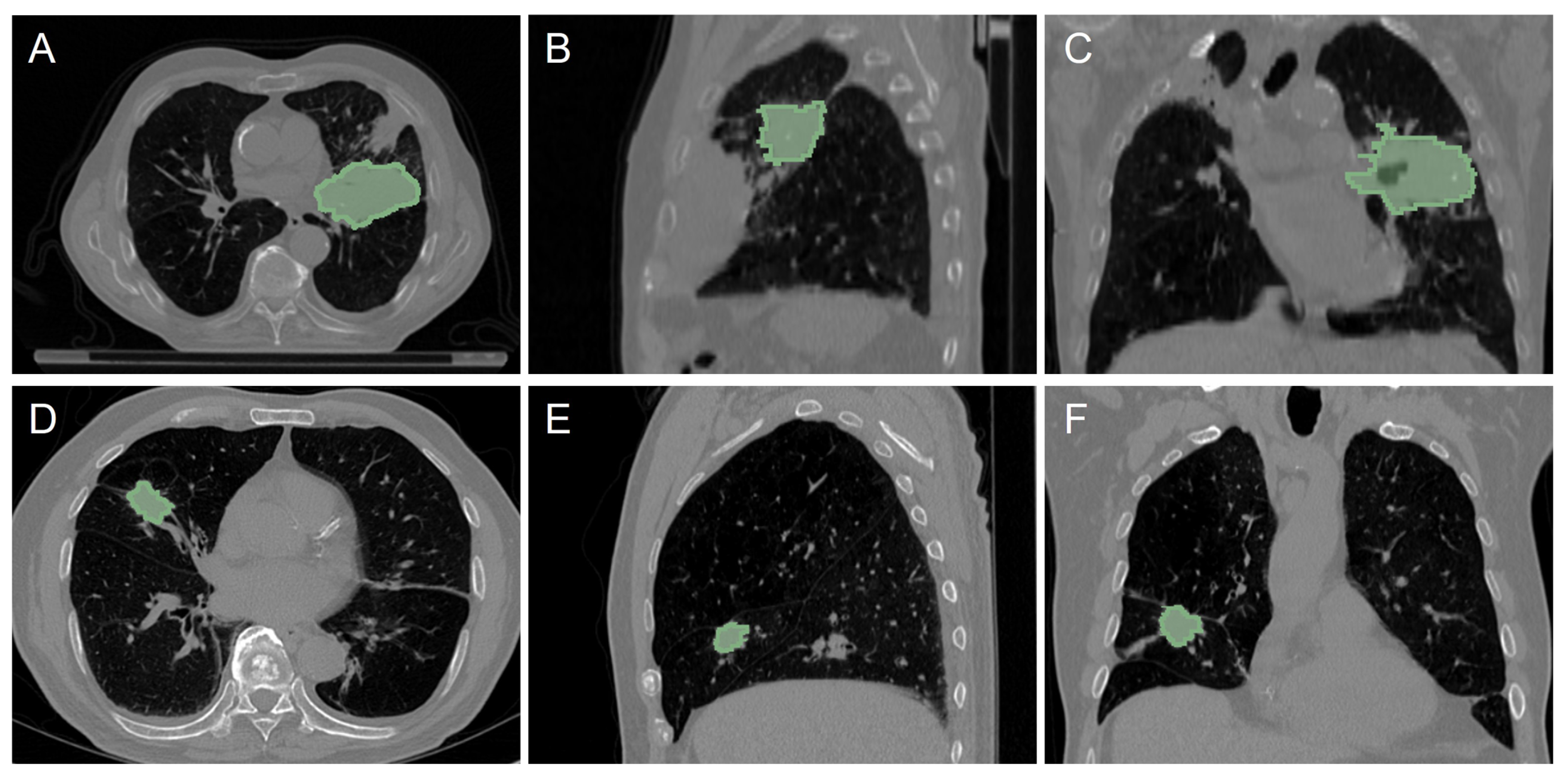
2.1. CT Dataset from NSCLC Patients

We utilized two publicly available NSCLC datasets from the TCIA repository [34]. The first was the TCIA-NSCLC Radiomics dataset (LUNG1), which included 422 patients treated at the MAASTRO Clinic in Maastricht, The Netherlands. The patients with inoperable, histologic, or cytologic confirmed NSCLC underwent FDG PET-CT acquisition for radiotherapy treatment planning using Siemens Biograph (SOMATOM Sensation-16 with an ECAT ACCEL PET scanner, Siemens Medical Solutions, Malvern, PA, USA). Patients were then treated with induction concurrent chemoradiotherapy, radiotherapy alone, or chemotherapy followed by radiotherapy. Additionally, the R01 cohort from the TCIA-NSCLC Radiogenomics dataset (LUNG2), which comprises 162 patients from the Stanford University School of Medicine and Palo Alto Veterans Affairs Healthcare System, was considered for external independent validation [32]. This dataset came from a retrospective study, where subjects were scanned using different scanners, protocols, and parameters. Similar to LUNG1, patients affected by NSCLC were treated with concurrent chemoradiotherapy, radiotherapy alone, or chemotherapy followed by radiotherapy. The original works provide specifics about patient recruitment and treatment.

Pre-treatment CT images and tumor contours manually delineated by experts are available from these datasets. In this study, a subset of patients was considered according to the following exclusion criteria:

• More than one tumor exists in the volume.
• The post-operative survival time was lower than two years, but the patient remained alive.
• There are misalignments or reading errors between CT images and tumor contours.

A total of 403 patients from LUNG1 and 130 patients from LUNG2 were thus finally considered. More details about CT images and patients’ clinical information are summarized in

Table 1. Parameters of CT images and patients from LUNG1 and LUNG2 datasets.

	LUNG1	LUNG2
Image parameters
Pixel size	$0.977\times 0.977$ mm2	$0.604\times 0.604$–$0.865\times 0.865$ mm2
Slice thickness	3.0 mm	0.8–3.0 mm
Patient information
Number of patients	403	130
Age (years)	68.2 ± 10.1	69.7 ± 8.6
Gender
Male	279 (69.2%)	98 (75.4%)
Female	124 (30.8%)	32 (24.6%)
Histology
Adenocarcinoma	47 (11.7%)	102 (78.5%)
Squamous Cell	149 (37.0%)	25 (19.2%)
Large Cell	108 (26.8%)	0 (0%)
Other	99 (24.6%)	3 (2.3%)
T stage
T1	88 (21.8%)	68 (52.3%)
T2	150 (37.2%)	44 (33.8%)
T3	49 (12.2%)	13 (10.0%)
T4	116 (28.8%)	5 (3.8%)
Median overall survival time (years)	1.5 ± 2.2	3.9 ± 1.8
Survival >2 years	161 (40.0%)	102 (78.5%)
Survival <2 years	242 (60.0%)	28 (21.5%)

, whereas illustrative examples of both datasets are shown in Figure 1. Additionally, patients were dichotomized into non-survivor and survivor based on their overall post-operative survival time, with a cut-off of two years, similar to the median survival time for these patients [9,35].

2.2. Radiomic Feature Extraction

One hundred and five classical radiomic features were computed within the tumor on the CT images using PyRadiomics open-source software (version 3.7.7) [36], implemented in Python and compliant with the Image Biomarker Standardization Initiative (IBSI) indications [7]. Specifically, the following features were extracted from the original non-filtered images: 14 shape features, 18 first-order statistics, 22 from the gray-level co-occurrence matrix (GLCM), 16 from the gray-level run-length matrix (GLRLM), 16 from the gray-level size-zone matrix (GLSZM), 14 from the gray-level dependence matrix (GLDM), and five from the neighboring gray-tone difference matrix (NGTDM).

Image intensities were discretized before computing texture matrices using a fixed bin width of 25, as suggested by the IBSI guidelines for CT intensity quantization [7]. Then, features were computed in the 3D space after resampling the images to isotropic voxels of $1\times 1\times 1$ mm.

Radiomic features are highly sensitive to differences in scan protocols; therefore, since LUNG1 and LUNG2 images came from different institutions, radiomic features may present different distributions due to the batch effect. Hence, a harmonization method was applied to the extracted radiomic features, a standard procedure in radiomics to increase model robustness [37]. Specifically, the BM-ComBat method, a modified version of the original ComBat method [38], allows transforming features to a reference batch (in this case, the LUNG1 dataset), using the Bayes theorem to estimate the scanner effect with a bootstrap strategy by matching the statistical distributions of the feature values without altering the biological information [37].

2.3. Proposed GP-Based Feature Construction Approach

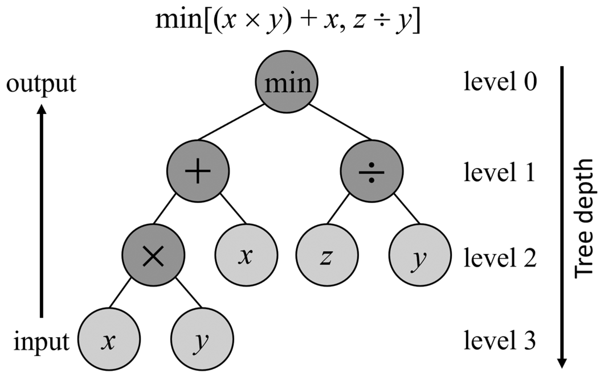
2.3.1. Genetic Programming Basics

Generally, the genetic algorithm (GA) is considered the main technique of the evolutionary computation paradigm, where potential solutions are codified into vectors called chromosomes [39]. On the other hand, genetic programming (GP) works similarly to GA, although the main difference lies in the type of encoding, which uses syntax trees instead of vectors. A tree intrinsically contains a computer program or mathematical expression [26]; hence, this property has been exploited to address the problem of automatic feature construction [27].

The GP codification requires defining a terminal set containing the problem’s independent variables and a function set containing mathematical functions and arithmetic operators. From both sets, an inverted tree-like representation is constructed in which leaf nodes are the inputs given by the terminal set, and inner nodes are the functions given by the function set that combine the inputs to generate an outcome in the root node at the top node. A didactic example is shown in Figure 2, where the terminal set is $\{x,y,z\}$, and the function set is $\{+,-,\times ,÷,\min ,\max \}$.

GP is a population-based metaheuristic in which the evolutionary process is enabled by the genetic operators of selection, crossover, and mutation applied to the population’s individuals. This way, the population evolves until reaching a predefined number of generations by minimizing (or maximizing) a fitness function determining the survival chances of every individual for the next generation [26].

The selection operator chooses individuals from the population based on their fitness. A common approach is selection by tournament, where two or more individuals are chosen randomly from the population, and the fittest individual is the winner and, therefore, selected.

The crossover operator simulates sexual reproduction in the natural world, where two selected individuals interchange their information to create offspring. This operator cuts an individual’s subtree at a random cut-off point and swaps it with another individual’s cut subtree. Hence, two children are generated that possess characteristics of both parents.

The mutation operator introduces a random change somewhere in a tree, which can be done using the subtree mutation strategy, where a cut-off point is randomly determined (similar to crossover), and the obtained subtree is replaced by a new randomly generated one.

Crossover and mutation operators are applied according to some probability, where crossover usually has the highest probability of occurrence.

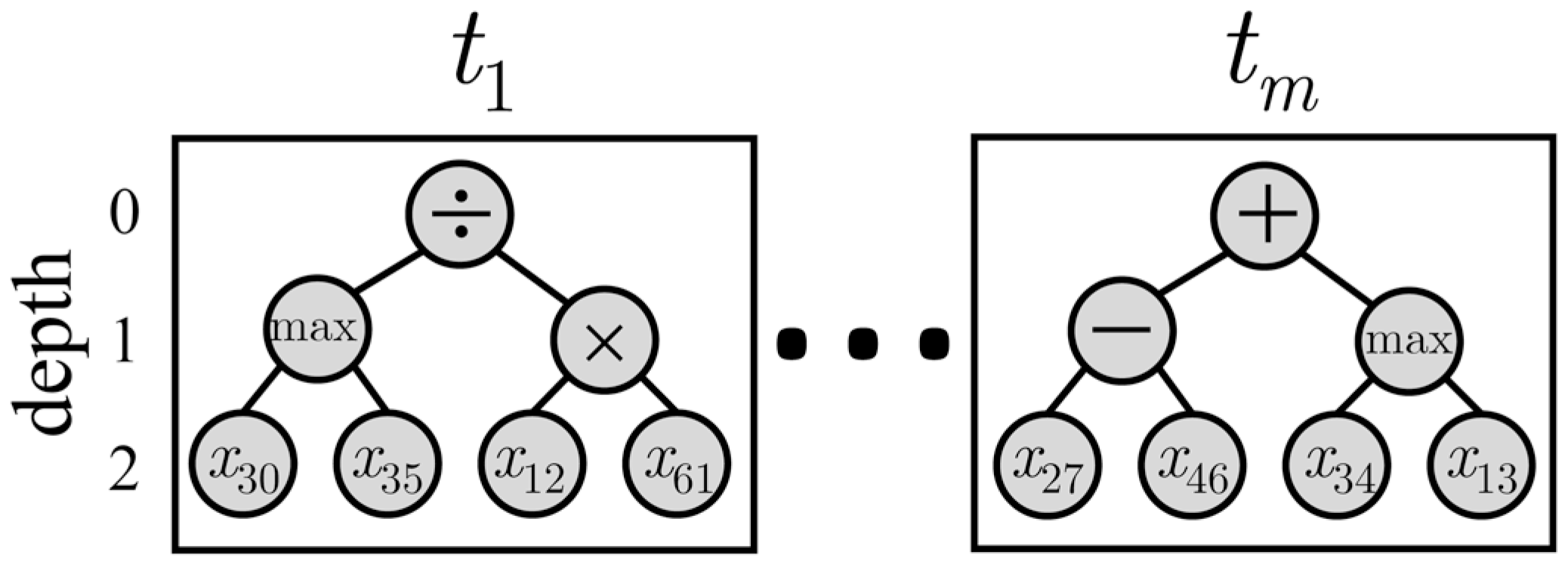
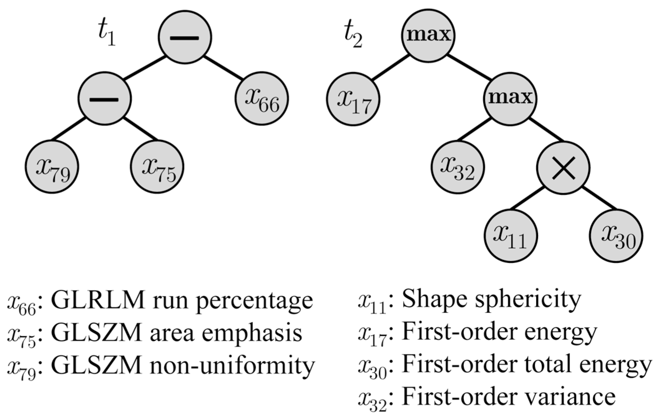
2.3.2. Multi-Tree Representation

The canonical GP algorithm encodes a potential solution in a single tree [26]; thus, only one feature can be constructed, risking a lack of separability between survivor and non-survivor class distributions. This issue can be overcome using a multi-tree representation to create a multi-dimensional feature space, in which a potential solution constructs a new feature set with m predictors from an original set with d features. We used the multi-tree representation proposed by [27], and Figure 3 illustrates this approach.

In a multi-tree representation, every tree is denoted by $t_j$ with $j=1,\dots ,m$, having a maximum depth $l_{\max }$, where a terminal node is an original radiomic feature, denoted by $x_i$ with $i=1,\dots ,d$. The inner nodes are arithmetic operators and mathematical functions that combine the inputs to construct a feature in the top node [27].

In short, the terminal set comprises 105 radiomic features depicted in Section 2.2. No constants are considered. The function set includes four arithmetic operators $\{+,-,\times ,÷\}$ and two order statistics operators $\{\min ,\max \}$. Among the four arithmetic operators, the first three work with their usual meaning. However, the division operator is protected; it returns $1.0$ if the denominator lies between $-0.001$ and $0.001$ [27].

2.3.3. Fitness Function

Usually, the fitness function for GP-based feature construction only assesses the classification performance obtained from the constructed features, i.e., at the trees’ outputs. However, the classification performance of the original radiomic feature set at the terminal nodes is ignored. Thus, it is possible to obtain solutions in which the constructed features may underperform the original ones. Aiming to ensure that constructed features improve the original radiomic features, we propose maximizing the classification performance gain output-to-input ratio, where the area under the ROC curve (AUC) evaluates the classification performance of two independent logistic regression (LR) classifiers trained with constructed and original radiomic features.

The AUC represents the probability that a given classifier correctly predicts an input from the positive class. Additionally, the majority class does not influence the AUC in class imbalance scenarios, such as survival prediction [40]. The Wilcoxon–Mann–Whitney test provides a direct estimator for AUC. Let ${\mathbf{p}}^{+}=[s_1^{+},\dots ,s_{n_{+}}^{+}]$ be the predicted scores of the positive class (i.e., non-survivor) with $n_{+}$ samples. Likewise, define ${\mathbf{p}}^{-}=[s_1^{-},\dots ,s_{n_{-}}^{-}]$ for the $n_{-}$ samples that belong to the negative class (i.e., survivors). Then, the combined set $\{{\mathbf{p}}^{-},{\mathbf{p}}^{+}\}$ is ranked in ascending order, and the AUC is calculated as [41]

$$\mathrm{AUC}={\displaystyle \frac{{\sum }_{i=1}^{n_{+}}{r}_i-n_{+}(n_{+}+1)/2}{n_{+}{n}_{-}}},$$

(1)

where $r_i$ is the rank of the ith sample belonging to the positive class. The AUC is bounded to the range $[0,1]$, where $0.5$ indicates a random classification, and $1.0$ is a perfect classification.

Let us denote ${\mathrm{AUC}}_{\mathrm{in}}$ and ${\mathrm{AUC}}_{\mathrm{out}}$ as the AUC values obtained with the original radiomic features at the terminal nodes and GP-constructed features at the output nodes, respectively. The AUC’s gain output-to-input ratio is expressed as

$$f\left(\mathbf{z}\right)={\displaystyle \frac{{\mathrm{AUC}}_{\mathrm{out}}}{{\mathrm{AUC}}_{\mathrm{in}}}},$$

(2)

where $\mathbf{z}=[t_1,\dots ,t_m]$ is a potential solution with multi-tree representation. To evaluate this fitness function, the AUC is trunked to the range $[0.5,1.0]$, so the fitness value ranges from 0.5 to 2.0; the higher the value, the better the gain. It is worth mentioning that several trees can share some radiomic features at the input nodes; thus, unrepeated features are considered to obtain ${\mathrm{AUC}}_{\mathrm{in}}$.

2.3.4. GP-Based Feature Construction Algorithm

Algorithm 1 shows the general feature construction pseudocode using GP [27]. This algorithm requires an input radiomic feature set, where each sample comprises 105 original radiomic features associated with an actual class label defined by non-survivor or survivor classes.

First, in line 1, the ramped half-and-half method creates the initial population, where each individual has m trees with maximum $l_{\max }$ levels [42]. Next, each individual’s fitness is calculated in line 6, where 5-fold cross-validation is used to split feature data into training and validation sets. The former is used for training two LR models (i.e., using original radiomic features and constructed ones), whereas the latter calculates ${\mathrm{AUC}}_{\mathrm{in}}$ and ${\mathrm{AUC}}_{\mathrm{out}}$; thus, the individual’s fitness is the mean fitness value in validation data. Notice that this strategy avoids prediction model overfitting.

Further, in line 11, the elite-preserving mechanism determines the next generation, where parents and offspring are merged and descendingly sorted according to their fitness. So, the first 50% of the sorted individuals are taken as the population for the next generation [43]. Finally, the algorithm’s output is the individual with the highest fitness value after $g_{\max }$ generations.

Algorithm 2 shows the pseudocode of crossover and mutation operators to create offspring in line 11 of Algorithm 1, where just one operator is executed according to a mutation probability $p_m\in (0,1)$. These two genetic operators evolve the population in the following manner: (i) crossover, where two individuals are selected for interchanging randomly selected subtrees to produce two new individuals, and (ii) mutation, where an individual is selected for replacing a randomly selected subtree with a randomly generated subtree to produce a new individual. Notice that in lines 2 and 7, the tournament selection method chooses one or two individuals for mutation or crossover. In lines 3 and 8, one tree is randomly picked from a selected individual to crossover or mutate.

It is worth mentioning that the crossover operator requires a crossover probability to bias the cut-off point to function or terminal nodes. Each selected individual then switches subtrees at their cut-off points. Usually, function nodes are more likely to be chosen as the crossover point than terminal nodes to avoid surpassing the maximum tree depth. If the size of a new individual exceeds the maximum allowed depth after the operation, it is excluded from the candidates to form the next generation. This criterion also applies to the mutation operator.

Algorithm 1 Feature construction using GP with multi-tree representation.

Input:  radiomic feature set; number of trees m; maximum tree depth $l_{\max }$; maximum number of generations $g_{\max }$ Output:  best individual ${\mathbf{z}}_{\mathrm{best}}$   1: Initialize population: each individual $\mathbf{z}$ has m trees with maximum $l_{\max }$ levels   2: ${\mathbf{z}}_{\mathrm{best}}$ is the first individual   3: while$g_{\max }$ is not reached do   4:     for all $\mathbf{z}$ in the population do   5:            Create a new feature set with m predictors from radiomic features   6:            Evaluate fitness function $f\left(\mathbf{z}\right)$                ▹ Equation (2)   7:            if $f\left(\mathbf{z}\right)>f\left({\mathbf{z}}_{\mathrm{best}}\right)$ then   8:                ${\mathbf{z}}_{\mathrm{best}}\leftarrow \mathbf{z}$                  ▹ Update the best individual   9:            end if 10:       end for 11:       Create the next generation using genetic operators         ▹ Algorithm 2 12: end while

The proposed GP-based approach was developed in MATLAB R2022b (The Mathworks, Boston, MA, USA), and the source codes are available at https://github.com/wgomezf/GP-radiomics (accessed on 4 August 2024).

Algorithm 2 Crossover and mutation operators.

1: if $\mathrm{rand}(0,1)<p_m$ then                       ▹ Mutation   2:      Select one individual $\mathbf{z}$ using tournament selection   3:      Select one tree t randomly from $\mathbf{z}$   4:      Select a subtree s in t randomly and replace it with a new subtree   5:      return one new individual   6: else                                ▹ Crossover   7:      Select two different individuals ${\mathbf{z}}_1$ and ${\mathbf{z}}_2$ using tournament selection   8:      Select two trees $t_1$ and $t_2$ randomly from ${\mathbf{z}}_1$ and ${\mathbf{z}}_2$, respectively   9:      Select two subtrees $s_1$ and $s_2$ randomly from $t_1$ and $t_2$ and swap them 10:      return two new individuals 11: end if

2.4. Experimental Setup

2.4.1. Benchmark Techniques

From now on, the proposed approach will be referred to as GP_GAIN, whose prediction performance was compared against four techniques from the literature: two feature selection methods widely used in radiomics to select a subset of original features and two GP-based feature construction methods with multi-tree representation that have already been used in other contexts but never applied to radiomics. Both feature selection and feature construction consider the filter and wrapper approaches, whose descriptions are reported in the following:

• FS_FWD is a wrapper feature selection approach based on sequential forward selection, where features are sequentially added to an empty set of features until adding extra features does not improve the AUC value of a logistic regression classifier [44].
• FS_mRMR is a filter feature selection technique based on the minimal redundancy–maximal relevance (mRMR) criterion, where dependencies between variables and class labels are measured with mutual information [45].
• GP_AUC is a GP-based wrapper feature construction method in which the fitness function is the AUC value obtained from a logistic regression classifier trained with the constructed features [40].
• GP_CORR is a GP-based filter feature construction method, where the Spearman correlation measures the redundancy between constructed features, while the relevance between features and class labels is calculated in terms of AUC. The fitness function is the difference between the relevance and redundancy averages [46].

The obtained feature sets from these approaches were used to train six classifiers: logistic regression (LR), linear discriminant analysis (LDA), naive Bayes (NB), random forest (RF), support vector machine with Gaussian kernel (SVM), and multilayer perceptron (MLP) [47]. Moreover, the hyperparameters of RF, MLP, and SVM classifiers were tuned by Bayesian optimization to determine the best prediction models [48].

Table 2. The classifier’s hyperparameter values.

Classifier	Hyperparameter	Value
RF	Features to sample	$\sqrt{d}$
	Decision trees	$[5,1000]$
	Leaf node samples	$[1,150]$
MLP	Hidden units	$[2,4\sqrt{d}]$
	Learning rate	$[{10}^{-6},{10}^{-2}]$
	Momentum factor	$[0.5,0.9]$
SVM	Margin penalty	$[2^{-5},2^5]$
	Gaussian bandwidth	$[2^{-5},2^5]$

d stands for the number of input features.

summarizes the hyperparameter ranges of these classifiers. Furthermore, the parameter settings used for the three GP-based approaches are summarized in

Table 3. The GP parameter settings.

Parameter	Value
Population size	50
Number of generations ($g_{\max }$)	100
Mutation probability ($p_m$)	0.10
Crossover probability ($p_c$)	0.90
Tournament size	5
Number of trees (m)	1 to 5
Maximum tree depth ($l_{\max }$)	2 to 7
Function set	$\{+,-,\times ,÷,\min ,\max \}$
Terminal set	105 radiomic features

.

2.4.2. Experiments

First, different GP_GAIN configurations were tested by varying the number of trees, m, from 1 to 5, and the depth levels, $l_{\max }$, from 2 to 7, using the 5-fold cross-validation method on the LUNG1 dataset. All the pairwise combinations of the number of trees and depth levels were assessed to identify the best configuration for survival prediction in NSCLC, where LR was the base classifier.

Next, two experiments were defined to evaluate the survival prediction of distinct prediction models. The first experiment is internal validation, which uses the LUNG1 dataset split into training and test sets using the 5-fold cross-validation method. This experiment aims to identify the best survival prediction models for feature selection and feature construction using distinct classifiers. The second experiment is external validation, which uses the entire LUNG2 dataset as a test set. This experiment aims to assess the generalization capabilities of the prediction models obtained in the first experiment using an independent test set external to the LUNG1 dataset.

The classification performance was evaluated regarding accuracy, precision, and recall, as summarized in

Table 4. The classification performance indices used to evaluate the methods.

Index	Expression
Accuracy	${\displaystyle \frac{\mathrm{TP}+\mathrm{TN}}{\mathrm{TP}+\mathrm{FN}+\mathrm{FP}+\mathrm{TN}}}$
Recall	${\displaystyle \frac{\mathrm{TP}}{\mathrm{TP}+\mathrm{FN}}}$
Precision	${\displaystyle \frac{\mathrm{TP}}{\mathrm{TP}+\mathrm{FP}}}$

. These indices were calculated from the binary confusion matrix $\left(\begin{array}{cc}\mathrm{TP}& \mathrm{FN}\\ \mathrm{FP}& \mathrm{TN}\end{array}\right)$, where TP is true positive, TN is true negative, FP is false positive, and FN is false negative. The AUC index in (1) also measured the separability between survivor and non-survivor predicted scores [49].

Survival analysis was also performed on LUNG1 and LUNG2 datasets, considering the best GP configuration and comparing the selected methods. First, the Kaplan–Meier (K–M) survival analysis is performed to associate the predicted binary classification with the survival information by splitting the survival curves into high- and low-risk groups. The log-rank test assesses significant differences between the two survival curves [50].

Next, the Cox proportional-hazards model was fitted considering the radiomic features selected by FS_FWD, FS_mRMR, and the constructed features obtained by the GP-based approaches. Also, age and tumor stage information were considered to adjust for potential confounding variables. As in previous works, C-Index was used as the evaluation metric for the Cox model [33,35].

To provide a quantitative tool that could be helpful in clinics and to enhance feature interpretability, a nomogram of the proposed approach was built based on multivariate logistic regression analysis in the training cohort by considering the best configuration for GP-based features, age, and TN tumor stage, as in [14].

3. Results

3.1. GP_GAIN Configurations

Table 5. The GP_GAIN method’s classification performance results for different configurations. The mean of five cross-validation experiments is presented. The best results are highlighted in bold.

Index	Tree Depth	Number of Trees
		1	2	3	4	5
AUC	2	0.68	0.66	0.66	0.66	0.65
	3	0.67	0.69	0.63	0.65	0.67
	4	0.65	0.67	0.68	0.66	0.65
	5	0.65	0.67	0.66	0.68	0.66
	6	0.69	0.65	0.66	0.63	0.67
	7	0.67	0.67	0.67	0.66	0.67
Accuracy	2	0.59	0.62	0.58	0.61	0.59
	3	0.61	0.65	0.59	0.59	0.61
	4	0.60	0.58	0.64	0.60	0.59
	5	0.61	0.60	0.62	0.61	0.60
	6	0.61	0.58	0.62	0.57	0.61
	7	0.61	0.59	0.60	0.62	0.62
Precision	2	0.49	0.52	0.48	0.50	0.47
	3	0.52	0.56	0.49	0.49	0.52
	4	0.50	0.48	0.54	0.50	0.49
	5	0.51	0.50	0.51	0.52	0.50
	6	0.51	0.46	0.51	0.46	0.51
	7	0.51	0.49	0.51	0.53	0.52
Recall	2	0.70	0.62	0.59	0.56	0.57
	3	0.69	0.61	0.60	0.65	0.50
	4	0.51	0.61	0.55	0.56	0.64
	5	0.61	0.61	0.58	0.52	0.66
	6	0.66	0.55	0.61	0.66	0.70
	7	0.59	0.65	0.62	0.61	0.67

summarizes the classification performance of the GP_GAIN method using different configurations. Noticeably, configurations with fewer shallow trees generally achieved higher classification performances. The best configuration used two trees and three depth levels, achieving the highest AUC of 0.69 and accuracy of 0.65. It also maintained an adequate balance between precision and recall. Thus, we selected this configuration for the internal and external validation experiments.

Figure 4 shows an example of two features constructed by the best GP_GAIN configuration obtained from one of the 5-fold cross-validation experiments. The first tree with two levels of depth constructs a new feature from three texture features; the second tree with three levels of depth combines shape and histogram features to construct a new feature. These two constructed features thus retain information from all three radiomic classes, i.e., shape, histogram-based, and texture features.

3.2. Internal Validation

Table 6. The benchmark techniques’ results using different classifiers on the LUNG1 dataset. The mean of five cross-validation experiments is presented. The best results are highlighted in bold.

Index	Method	LR	LDA	NB	RF	SVM	MLP
AUC	FS_mRMR	0.63	0.62	0.61	0.64	0.65	0.62
	FS_FWD	0.65	0.65	0.63	0.60	0.66	0.63
	GP_AUC	0.61	0.61	0.62	0.61	0.60	0.60
	GP_CORR	0.67	0.63	0.65	0.62	0.59	0.63
	GP_GAIN	0.69	0.68	0.70	0.64	0.68	0.67
Accuracy	FS_mRMR	0.57	0.57	0.59	0.62	0.57	0.58
	FS_FWD	0.62	0.60	0.60	0.56	0.60	0.58
	GP_AUC	0.56	0.55	0.57	0.56	0.54	0.55
	GP_CORR	0.60	0.57	0.58	0.58	0.56	0.58
	GP_GAIN	0.65	0.65	0.64	0.59	0.62	0.64
Precision	FS_mRMR	0.47	0.46	0.48	0.53	0.49	0.48
	FS_FWD	0.52	0.50	0.50	0.46	0.49	0.48
	GP_AUC	0.47	0.46	0.48	0.45	0.45	0.45
	GP_CORR	0.50	0.47	0.48	0.48	0.46	0.47
	GP_GAIN	0.56	0.55	0.55	0.39	0.52	0.54
Recall	FS_mRMR	0.52	0.52	0.65	0.56	0.61	0.63
	FS_FWD	0.65	0.61	0.52	0.56	0.63	0.51
	GP_AUC	0.62	0.64	0.61	0.63	0.71	0.63
	GP_CORR	0.60	0.55	0.63	0.62	0.52	0.55
	GP_GAIN	0.61	0.59	0.63	0.53	0.59	0.61
K–M ($\times {10}^{-3}$)	FS_mRMR	149.829	92.688	0.538	3.188	18.356	0.230
	FS_FWD	0.001	0.311	2.041	33.303	0.020	4.625
	GP_AUC	1.834	2.291	0.267	2.247	5.895	19.451
	GP_CORR	6.176	136.507	28.744	28.731	277.792	83.912
	GP_GAIN	0.012	0.205	0.000	2.116	0.951	0.019

shows the results of the internal validation on the LUNG1 dataset, comparing the classification performance of different feature selection and feature construction methods. For this analysis, the three GP-based models used the best GP_GAIN configuration found previously, i.e., a maximum depth of three levels and two trees; this way, they all have the same configuration to construct two new features. Regarding feature selection methods, FS_FWD and FS_mRMR selected, on average, six and thirteen original radiomic features, respectively.

Notably, classification models trained with GP_GAIN-based features achieved the highest AUC and accuracy values in every classifier, with LR, LDA, and NB performing the best (AUC equal to 0.69, 0.68, and 0.70, and accuracy equal to 0.65, 0.65, and 0.64, respectively). By observing the K–M survival analysis, the log-rank test revealed that the curves between survival and non-survival patients significantly differed between the two groups, with NB achieving the lowest p-value ($9.2\times {10}^{-7}$). In the first column of

Table 7. The C-index results of the Cox proportional-hazards models considering age, tumor stage, and features selected by each method.

	Dataset
Method	LUNG1	LUNG2
FS-mRMR	0.608	0.692
FS-SFS-FWD	0.606	0.643
GP-AUC	0.601	0.639
GP-CORR	0.579	0.659
GP-GAIN	0.586	0.644

, results of the Cox model are reported for the LUNG1 dataset, with the C-index ranging from 0.58 to 0.61, showing a moderate ability to predict survival time.

3.3. External Validation

Finally, the external validation results performed on the LUNG2 dataset are summarized in

Table 8. The benchmark techniques’ results using different classifiers on the LUNG2 dataset. The mean of five cross-validation experiments is presented. The best results are highlighted in bold.

Index	Method	LR	LDA	NB	RF	SVM	MLP
AUC	FS_mRMR	0.65	0.66	0.59	0.66	0.65	0.62
	FS_FWD	0.65	0.65	0.65	0.58	0.67	0.62
	GP_AUC	0.65	0.65	0.65	0.65	0.65	0.65
	GP_CORR	0.69	0.69	0.69	0.65	0.71	0.67
	GP_GAIN	0.68	0.68	0.63	0.68	0.67	0.67
Accuracy	FS_mRMR	0.63	0.64	0.52	0.39	0.64	0.69
	FS_FWD	0.66	0.56	0.61	0.52	0.65	0.64
	GP_AUC	0.58	0.58	0.58	0.62	0.58	0.58
	GP_CORR	0.58	0.58	0.58	0.62	0.55	0.54
	GP_GAIN	0.74	0.68	0.65	0.74	0.54	0.74
Precision	FS_mRMR	0.86	0.86	0.80	0.87	0.84	0.83
	FS_FWD	0.87	0.87	0.86	0.83	0.85	0.83
	GP_AUC	0.86	0.86	0.86	0.87	0.88	0.88
	GP_CORR	0.89	0.89	0.89	0.83	0.89	0.92
	GP_GAIN	0.85	0.87	0.86	0.82	0.88	0.84
Recall	FS_mRMR	0.63	0.65	0.52	0.26	0.67	0.76
	FS_FWD	0.67	0.52	0.60	0.49	0.68	0.68
	GP_AUC	0.56	0.56	0.56	0.60	0.55	0.55
	GP_CORR	0.54	0.54	0.54	0.65	0.48	0.45
	GP_GAIN	0.81	0.70	0.66	0.85	0.48	0.82
K–M ($\times {10}^{-2}$)	FS_mRMR	1.67	1.77	7.46	42.23	5.88	6.73
	FS_FWD	0.03	1.94	1.02	22.75	0.77	1.33
	GP_AUC	0.20	0.20	0.20	0.09	0.05	0.05
	GP_CORR	1.75	1.75	0.66	18.77	5.16	5.23
	GP_GAIN	2.65	1.93	0.61	8.58	13.28	0.84

. In this case, GP_CORR outperformed the other methods in terms of AUC (range 0.65–0.69 for the different classifiers), whereas GP_GAIN was the best for accuracy (range 0.65–0.74) and the second best for AUC (range 0.63–0.68). Nonetheless, GP_GAIN presented the most balanced combination of precision and recall. Feature selection approaches achieved the lowest classification performance, especially for NB, RF, and MLP classifiers.

The K–M survival analysis showed that GP_AUC reached the lowest p-values; the curves between survival and non-survival groups were significantly different in almost all cases except for the RF classifier. Moreover, for the LUNG2 dataset, the Cox model revealed higher C-index values than LUNG1, in the range of 0.64–0.69, as shown in the second column of Table 7.

4. Discussion

This paper proposed a GP-based feature construction approach to build new discriminant features for survival prediction in NSCLC patients. A multi-tree representation was used to build a new multi-dimensional feature space from traditional radiomic features, including morphological, volumetric, histogram-based, and texture parameters computed from CT images. The main contribution is applying GP for feature construction in radiomics for the first time to improve the survival prediction of NSCLC patients. The comparison with benchmark methods showed that classification models built from GP features generally outperform traditional feature selection methods for most considered classifiers concerning internal and external validations, confirming its generalizability. In addition, the AUC-based fitness function, which measures the output-to-input AUC gain, guided the GP algorithm to find more accurate solutions than its GP counterparts, especially in the LUNG1 dataset.

The differences in classification performances between the internal and external validations can be explained by the different class proportions of the two datasets. The LUNG1 dataset was almost balanced, with 40% of patients surviving more than two years; on the contrary, the LUNG2 dataset was highly unbalanced since almost 80% of patients had a survival higher than two years. This behavior can justify the higher precision values in the second dataset. In this case, GP_GAIN showed the highest values for recall compared to the other methods, making the classification performances more balanced.

The experimental results showed relatively low classification performance by all the assessed approaches, suggesting that predicting the two-year survival of NSCLC patients is challenging. Examining the K-M survival curves and the Cox model results, none of the radiomic approaches can give satisfactory results. In particular, the FS_mRMR method achieved the highest C-index, probably due to the larger number of selected features that can better model the survival time. Nevertheless, this approach was the worst in terms of classification performance.

As shown in

Table 9. The comparison of distinct related works to predict the two-year survival of NSCLC patients using the LUNG1 (L1) and LUNG2 (L2) datasets. The suffixes T and V indicate whether the dataset was used for training or validation. The radiomics and deep learning approaches are denoted as R and DL, respectively.

Reference	Approach	Dataset	Main Result
[9]	Radiomics	L1-T L2-V	AUC = 0.65–0.66
[12]	Radiomics	L1-T, V	AUC = 0.76 for TNM stage I group
[16]	Radiomics and DL	L1-T, V	C-index = 0.623 for R + DL C-index = 0.585 for DL
[13]	Radiomics	L1-T L2-V	AUC = 0.61
[33]	Radiomics	L1-T	C-index = 0.60
[11]	Radiomics and DL	L1-T, V	AUC = 0.67 for R AUC = 0.63 for DL AUC = 0.67 for R + DL
[14]	Radiomics	L1-T Other-V	C-index = 0.62–0.73
Ours	GP-based radiomics	L1-T L2-V	AUC = 0.71, C-index = 0.66

, related works in the literature that used traditional radiomic features to predict NSCLC two-year survival obtained similar or even lower results than our GP_GAIN approach. These studies utilized LUNG1 and LUNG2 datasets, so we can directly compare our results with these approaches. The AUC values informed by [35] were 0.65–0.67, and those reported by [9] were 0.54–0.66, whereas GP_GAIN achieved 0.64–0.70. In a recent study, Braghetto et al. [11] demonstrated that all the studies adopting the LUNG1 dataset to assess the ability of radiomics to predict two-year survival presented AUC values in the range of 0.61–0.66. Also, Chaddad et al. [12] included clinical information and increased the two-year survival prediction performance if the population was separately analyzed by considering tumor subtypes and stage groups. In this case, a higher prediction performance (AUC = 0.76) was achieved for patients in Stage I of the TNM (Tumor, Node, Metastasis) system.

The AUC differences between previous works and our approach indicate that traditional radiomic features could not fully stratify NSCLC patients. However, constructing new GP-based features can improve the classification performance [51]. This behavior can also be confirmed by comparing GP_GAIN with two feature selection methods that selected a subset of original radiomic features: the minimal redundancy–maximal relevance method (AUC was 0.61–0.65) and the sequential forward selection method (AUC was 0.60–0.66).

On the other hand, as indicated in Table 9, deep learning models obtained C-index and AUC values within the same range as, or even lower than, those obtained by traditional radiomic models. Therefore, learning deep features did not notably improve the prognostic power of radiomic models since CNNs require large training datasets to improve generalization [11], though LUNG1 is a small-sized dataset. Furthermore, CNN models are black-box models since interpreting why a particular prediction is made can be difficult [52]. In contrast, GP-based feature construction naturally produces an analytical human-readable expression represented as a tree structure, where terminal nodes select radiomic features combined with mathematical operators.

Moreover, the two-year survival prediction performance improvement by the proposed GP-based approach is due to its ability to maximize the AUC output-to-input ratio. This way, the AUC value is expected to be higher with constructed features at the trees’ top nodes (i.e., outputs) than the original radiomic features at the trees’ terminal nodes (i.e., inputs). Therefore, the GP_GAIN fitness function outperformed GP_AUC, which maximized the output AUC value (AUC was 0.60–0.62) and GP_CORR, where the fitness function measured the relevancy–redundancy of constructed features (AUC was 0.59–0.67).

It is worth mentioning that GP_GAIN trains two classifiers when the fitness function is evaluated: an LR model with original features at the trees’ input and another LR model with created features at the trees’ output. Hence, a limitation is that the computation time can be higher than GP_AUC and GP_CORR, mainly when the number of depth levels increases: the higher the depth levels, the more numerous the terminal nodes (i.e., original features to train an LR model). Nevertheless, solutions using a few shallow trees obtained the best classification performance. Indeed, the best model used two trees with a maximum of three depth levels, shown in Figure 4, suggesting that shallow trees tend to construct more generalizable features. Moreover, these two constructed features combined indices from all the radiomic classes (i.e., shape, histogram-based, and texture features), thus highlighting the relevance of different sources in the final classification. This observation aligns with the most recent works that proposed radiomic signatures that enclose different radiomic features for the survival prediction of NSCLC patients using traditional ML methods [53,54].

Another limitation of our work is that the two datasets (LUNG1 and LUNG2) used for training and testing present intrinsic differences in patients’ characteristics, thus limiting the effectiveness of the comparison and the generalizability of our approach. Nonetheless, the availability of these two datasets, which have been widely adopted in the literature to train and test different approaches, makes it possible to compare directly with previous works.

The proposed approach has several potential benefits for clinical practice. It offers improved predictive performance for two-year survival, better generalizability across different datasets, and greater robustness compared to traditional radiomics. Additionally, to make it easier for clinicians to understand and use, GP-based features can be utilized to create nomograms, which oncologists commonly use to make decisions. This approach has been widely employed in radiomics to predict survival in NSCLC [14]. Figure 5 shows a nomogram created using the best GP-based features and clinical and demographic information (such as age and T and N stages). Survival probability was estimated from the LR classifier. This approach enables NSCLC patients to receive information about clinical decision-making and personalized treatment options using traditional tools like nomograms enhanced by informative, independent, and reliable GP features.

5. Conclusions

This work proposed a GP-based radiomic model for the survival prediction of patients affected by NSCLC. This method constructed new relevant and independent features from original radiomic parameters by maximizing a fitness function that measured the classification performance gain using the output-to-input AUC ratio. This approach was compared with other techniques traditionally used in radiomic feature selection and GP-based methods.

The experimental results revealed that the proposed method increased survival prediction performance, even using challenging data like the LUNG1 dataset. Therefore, it could potentially support oncologists in determining the clinical prognosis of patients with lung cancer, with personalized treatment planning and prognosis to improve patients’ outcomes. A practical application that could enhance the impact of the proposed work in clinics would be integrating GP-based signatures in a nomogram.

Future work considers learning GP features directly from the original input images. The idea is to learn subtle features that classical radiomic features can miss. This approach has been tested on natural images with competitive results regarding deep neural networks [55]. On the other hand, our study revealed that less complex models (i.e., shallow trees) achieved better prediction performance. Hence, another research direction is to address feature construction as a multiobjective optimization problem to minimize simultaneously the error rate and the model’s complexity. Hence, a Pareto front is obtained, providing different tradeoffs between the two objectives [55]. Finally, GP-based radiomics will be evaluated on other oncological applications, such as breast or prostate cancer, to test and claim the wider generalizability of the proposed approach.

References

1. Sung, H.; Ferlay, J.; Siegel, R.L.; Laversanne, M.; Soerjomataram, I.; Jemal, A.; Bray, F. Global Cancer Statistics 2020: GLOBOCAN Estimates of Incidence and Mortality Worldwide for 36 Cancers in 185 Countries. CA Cancer J. Clin. 2021, 71, 209–249. [Google Scholar] [CrossRef] [PubMed]
2. Vo, T.H.; Lee, G.S.; Yang, H.J.; Oh, I.J.; Kim, S.H.; Kang, S.R. Survival Prediction of Lung Cancer Using Small-Size Clinical Data with a Multiple Task Variational Autoencoder. Electronics 2021, 10, 1396. [Google Scholar] [CrossRef]
3. Yang, Y.; Xu, L.; Sun, L.; Zhang, P.; Farid, S.S. Machine learning application in personalised lung cancer recurrence and survivability prediction. Comput. Struct. Biotechnol. J. 2022, 20, 1811–1820. [Google Scholar] [CrossRef] [PubMed]
4. Ahsan, M.M.; Luna, S.A.; Siddique, Z. Machine-Learning-Based Disease Diagnosis: A Comprehensive Review. Healthcare 2022, 10, 541. [Google Scholar] [CrossRef] [PubMed]
5. Scalco, E.; Rizzo, G.; Mastropietro, A. The stability of oncologic MRI radiomic features and the potential role of deep learning: A review. Phys. Med. Biol. 2022, 67, 09TR03. [Google Scholar] [CrossRef] [PubMed]
6. Scalco, E.; Rizzo, G. Texture analysis of medical images for radiotherapy applications. Br. J. Radiol. 2017, 90, 20160642. [Google Scholar] [CrossRef] [PubMed]
7. Zwanenburg, A.; Vallières, M.; Abdalah, M.A.; Aerts, H.J.; Andrearczyk, V.; Apte, A.; Ashrafinia, S.; Bakas, S.; Beukinga, R.J.; Boellaard, R.; et al. The Image Biomarker Standardization Initiative: Standardized Quantitative Radiomics for High-Throughput Image-based Phenotyping. Radiology 2020, 295, 328–338. [Google Scholar] [CrossRef] [PubMed]
8. Scrivener, M.; de Jong, E.E.; van Timmeren, J.E.; Pieters, T.; Ghaye, B.; Geets, X. Radiomics applied to lung cancer: A review. Transl. Cancer Res. 2016, 5, 398–409. [Google Scholar] [CrossRef]
9. Parmar, C.; Grossmann, P.; Bussink, J.; Lambin, P.; Aerts, H.J.W.L. Machine Learning methods for Quantitative Radiomic Biomarkers. Sci. Rep. 2015, 5, 13087. [Google Scholar] [CrossRef]
10. Zhang, Y.; Oikonomou, A.; Wong, A.; Haider, M.A.; Khalvati, F. Radiomics-based Prognosis Analysis for Non-Small Cell Lung Cancer. Sci. Rep. 2017, 7, 46349. [Google Scholar] [CrossRef]
11. Braghetto, A.; Marturano, F.; Paiusco, M.; Baiesi, M.; Bettinelli, A. Radiomics and deep learning methods for the prediction of 2-year overall survival in LUNG1 dataset. Sci. Rep. 2022, 12, 14132. [Google Scholar] [CrossRef] [PubMed]
12. Chaddad, A.; Desrosiers, C.; Toews, M.; Abdulkarim, B. Predicting survival time of lung cancer patients using radiomic analysis. Oncotarget 2017, 8, 104393. [Google Scholar] [CrossRef] [PubMed]
13. Shi, Z.; Zhovannik, I.; Traverso, A.; Dankers, F.J.; Deist, T.M.; Kalendralis, P.; Monshouwer, R.; Bussink, J.; Fijten, R.; Aerts, H.J.; et al. Distributed radiomics as a signature validation study using the Personal Health Train infrastructure. Sci. Data 2019, 6, 218. [Google Scholar] [CrossRef] [PubMed]
14. Yang, L.; Yang, J.; Zhou, X.; Huang, L.; Zhao, W.; Wang, T.; Zhuang, J.; Tian, J. Development of a radiomics nomogram based on the 2D and 3D CT features to predict the survival of non-small cell lung cancer patients. Eur. Radiol. 2019, 29, 2196–2206. [Google Scholar] [CrossRef] [PubMed]
15. Yadav, S.S.; Jadhav, S.M. Deep convolutional neural network based medical image classification for disease diagnosis. J. Big Data 2019, 6, 113. [Google Scholar] [CrossRef]
16. Haarburger, C.; Weitz, P.; Rippel, O.; Merhof, D. Image-based survival prediction for lung cancer patients using CNNS. In Proceedings of the 2019 IEEE 16th International Symposium on Biomedical Imaging (ISBI 2019), Venice, Italy, 8–11 April 2019; pp. 1197–1201. [Google Scholar] [CrossRef]
17. Hosny, A.; Parmar, C.; Coroller, T.P.; Grossmann, P.; Zeleznik, R.; Kumar, A.; Bussink, J.; Gillies, R.J.; Mak, R.H.; Aerts, H.J. Deep learning for lung cancer prognostication: A retrospective multi-cohort radiomics study. PLoS Med. 2018, 15, e1002711. [Google Scholar] [CrossRef] [PubMed]
18. O’Mahony, N.; Campbell, S.; Carvalho, A.; Harapanahalli, S.; Hernandez, G.V.; Krpalkova, L.; Riordan, D.; Walsh, J. Deep Learning vs. Traditional Computer Vision. In Proceedings of the Advances in Computer Vision, Las Vegas, NV, USA, 2–3 May 2019; pp. 128–144. [Google Scholar] [CrossRef]
19. Devarriya, D.; Gulati, C.; Mansharamani, V.; Sakalle, A.; Bhardwaj, A. Unbalanced breast cancer data classification using novel fitness functions in genetic programming. Expert Syst. Appl. 2020, 140, 112866. [Google Scholar] [CrossRef]
20. Ain, Q.U.; Al-Sahaf, H.; Xue, B.; Zhang, M. A genetic programming approach to feature construction for ensemble learning in skin cancer detection. In Proceedings of the 2020 Genetic and Evolutionary Computation Conference. Association for Computing Machinery, 2020, GECCO ‘20, Cancún, Mexico, 8–12 July 2020; pp. 1186–1194. [Google Scholar] [CrossRef]
21. Vanneschi, L. Machine Learning for Survival Prediction in Breast Cancer; NOVA IMS: Lisboa, Portugal, 2021. [Google Scholar]
22. Ain, Q.U.; Al-Sahaf, H.; Xue, B.; Zhang, M. Genetic programming for automatic skin cancer image classification. Expert Syst. Appl. 2022, 197, 116680. [Google Scholar] [CrossRef]
23. Sattar, M.; Majid, A.; Kausar, N.; Bilal, M.; Kashif, M. Lung cancer prediction using multi-gene genetic programming by selecting automatic features from amino acid sequences. Comput. Biol. Chem. 2022, 98, 107638. [Google Scholar] [CrossRef] [PubMed]
24. Ochoa-Montiel, R.; Sossa, H.; Olague, G.; Sánchez-López, C. Machine Learning and Symbolic Learning for the Recognition of Leukemia L1, L2 and L3. In Proceedings of the Pattern Recognition; Vergara-Villegas, O.O., Cruz-Sánchez, V.G., Sossa-Azuela, J.H., Carrasco-Ochoa, J.A., Martínez-Trinidad, J.F., Olvera-López, J.A., Eds.; Springer: Cham, Switzerland, 2022; pp. 360–369. [Google Scholar] [CrossRef]
25. Olson, R.S.; Urbanowicz, R.J.; Andrews, P.C.; Lavender, N.A.; Kidd, L.C.; Moore, J.H. Automating Biomedical Data Science Through Tree-Based Pipeline Optimization. In Proceedings of the Applications of Evolutionary Computation; Squillero, G., Burelli, P., Eds.; Springer: Cham, Switzerland, 2016; pp. 123–137. [Google Scholar] [CrossRef]
26. Poli, R.; Koza, J.R. Genetic Programming. In Search Methodologies: Introductory Tutorials in Optimization and Decision Support Techniques; Burke, E.K., Kendall, G., Eds.; Springer: Boston, MA, USA, 2005; pp. 127–164. [Google Scholar] [CrossRef]
27. Tran, B.; Xue, B.; Zhang, M. Genetic programming for multiple-feature construction on high-dimensional classification. Pattern Recognit. 2019, 93, 404–417. [Google Scholar] [CrossRef]
28. Ain, Q.U.; Al-Sahaf, H.; Xue, B.; Zhang, M. A Multi-tree Genetic Programming Representation for Melanoma Detection Using Local and Global Features. In Proceedings of the AI 2018: Advances in Artificial Intelligence, Wellington, New Zealand, 11–14 December 2018; Springer: Cham, Switzerland, 2018; pp. 111–123. [Google Scholar] [CrossRef]
29. Bhardwaj, H.; Sakalle, A.; Tiwari, A.; Verma, M.; Bhardwaj, A. Breast Cancer Diagnosis using Simultaneous Feature Selection and Classification: A Genetic Programming Approach. In Proceedings of the 2018 IEEE Symposium Series on Computational Intelligence (SSCI), Bangalore, India, 18–21 November 2018; pp. 2186–2192. [Google Scholar] [CrossRef]
30. Scalco, E.; Rizzo, G.; Gómez-Flores, W. Automatic Feature Construction Based on Genetic Programming for Survival Prediction in Lung Cancer Using CT Images. In Proceedings of the 2022 44th Annual International Conference of the IEEE Engineering in Medicine & Biology Society (EMBC), Glasgow, UK, 11–15 July 2022; pp. 3797–3800. [Google Scholar] [CrossRef]
31. Aerts, H.J.; Velazquez, E.R.; Leijenaar, R.T.; Parmar, C.; Grossmann, P.; Carvalho, S.; Bussink, J.; Monshouwer, R.; Haibe-Kains, B.; Rietveld, D.; et al. Decoding tumour phenotype by noninvasive imaging using a quantitative radiomics approach. Nat. Commun. 2014, 5, 4006. [Google Scholar] [CrossRef] [PubMed]
32. Bakr, S.; Gevaert, O.; Echegaray, S.; Ayers, K.; Zhou, M.; Shafiq, M.; Zheng, H.; Benson, J.A.; Zhang, W.; Leung, A.N.; et al. A radiogenomic dataset of non-small cell lung cancer. Sci. Data 2018, 5, 1–9. [Google Scholar] [CrossRef] [PubMed]
33. Welch, M.L.; McIntosh, C.; Haibe-Kains, B.; Milosevic, M.F.; Wee, L.; Dekker, A.; Huang, S.H.; Purdie, T.G.; O’Sullivan, B.; Aerts, H.J.; et al. Vulnerabilities of radiomic signature development: The need for safeguards. Radiother. Oncol. 2019, 130, 2–9. [Google Scholar] [CrossRef] [PubMed]
34. Clark, K.; Vendt, B.; Smith, K.; Freymann, J.; Kirby, J.; Koppel, P.; Moore, S.; Phillips, S.; Maffitt, D.; Pringle, M.; et al. The Cancer Imaging Archive (TCIA): Maintaining and operating a public information repository. J. Digit. Imaging 2013, 26, 1045–1057. [Google Scholar] [CrossRef] [PubMed]
35. Shen, C.; Liu, Z.; Guan, M.; Song, J.; Lian, Y.; Wang, S.; Tang, Z.; Dong, D.; Kong, L.; Wang, M.; et al. 2D and 3D CT Radiomics Features Prognostic Performance Comparison in Non-Small Cell Lung Cancer. Transl. Oncol. 2017, 10, 886–894. [Google Scholar] [CrossRef] [PubMed]
36. Van Griethuysen, J.J.; Fedorov, A.; Parmar, C.; Hosny, A.; Aucoin, N.; Narayan, V.; Beets-Tan, R.G.; Fillion-Robin, J.C.; Pieper, S.; Aerts, H.J.W.L. Computational radiomics system to decode the radiographic phenotype. Cancer Res. 2017, 77, e104–e107. [Google Scholar] [CrossRef] [PubMed]
37. Da-Ano, R.; Masson, I.; Lucia, F.; Doré, M.; Robin, P.; Alfieri, J.; Rousseau, C.; Mervoyer, A.; Reinhold, C.; Castelli, J.; et al. Performance comparison of modified ComBat for harmonization of radiomic features for multicenter studies. Sci. Rep. 2020, 10, 10248. [Google Scholar] [CrossRef]
38. Fortin, J.P.; Parker, D.; Tunç, B.; Watanabe, T.; Elliott, M.A.; Ruparel, K.; Roalf, D.R.; Satterthwaite, T.D.; Gur, R.C.; Gur, R.E.; et al. Harmonization of multi-site diffusion tensor imaging data. Neuroimage 2017, 161, 149–170. [Google Scholar] [CrossRef] [PubMed]
39. Engelbrecht, A.P. Computational Intelligence, 1st ed.; John Wiley & Sons: Hoboken, NJ, USA, 2007. [Google Scholar]
40. Pei, W.; Xue, B.; Shang, L.; Zhang, M. Genetic programming for high-dimensional imbalanced classification with a new fitness function and program reuse mechanism. Soft Comput. 2020, 45, 18021–18038. [Google Scholar] [CrossRef]
41. Hand, D.J.; Till, R.J. A Simple Generalisation of the Area Under the ROC Curve for Multiple Class Classification Problems. Mach. Learn. 2001, 45, 171–186. [Google Scholar] [CrossRef]
42. Luke, S.; Panait, L. A Survey and Comparison of Tree Generation Algorithms. In Proceedings of the 3rd Annual Conference on Genetic and Evolutionary Computation, GECCO’01, San Francisco, CA, USA, 7–11 July 2001; pp. 81–88. [Google Scholar]
43. Deb, K.; Pratap, A.; Agarwal, S.; Meyarivan, T. A fast and elitist multiobjective genetic algorithm: NSGA-II. IEEE Trans. Evol. Comput. 2002, 6, 182–197. [Google Scholar] [CrossRef]
44. Massafra, R.; Bove, S.; Lorusso, V.; Biafora, A.; Comes, M.C.; Didonna, V.; Diotaiuti, S.; Fanizzi, A.; Nardone, A.; Nolasco, A.; et al. Radiomic Feature Reduction Approach to Predict Breast Cancer by Contrast-Enhanced Spectral Mammography Images. Diagnostics 2021, 11, 684. [Google Scholar] [CrossRef] [PubMed]
45. Peng, H.; Long, F.; Ding, C. Feature selection based on mutual information criteria of max-dependency, max-relevance, and min-redundancy. IEEE Trans. Pattern Anal. Mach. Intell. 2005, 27, 1226–1238. [Google Scholar] [CrossRef] [PubMed]
46. Wang, R.; Tang, K. Feature Selection for Maximizing the Area Under the ROC Curve. In Proceedings of the 2009 IEEE International Conference on Data Mining Workshops, Miami, FL, USA, 6 December 2009; pp. 400–405. [Google Scholar] [CrossRef]
47. Duda, R.O.; Hart, P.E.; Stork, D.G. Pattern Classification, 2nd ed.; John Wiley & Sons: Hoboken, NJ, USA, 2001. [Google Scholar]
48. Wu, J.; Chen, X.Y.; Zhang, H.; Xiong, L.D.; Lei, H.; Deng, S.H. Hyperparameter Optimization for Machine Learning Models Based on Bayesian Optimization. J. Electron. Sci. Technol. 2019, 17, 26–40. [Google Scholar] [CrossRef]
49. Sokolova, M.; Lapalme, G. A systematic analysis of performance measures for classification tasks. Inform. Process. Manag. 2009, 45, 427–437. [Google Scholar] [CrossRef]
50. Goel, M.K.; Khanna, P.; Kishore, J. Understanding survival analysis: Kaplan-Meier estimate. Int. J. Ayurveda Res. 2010, 1, 274–278. [Google Scholar] [CrossRef] [PubMed]
51. Wang, X.; Duan, H.; Li, X.; Ye, X.; Huang, G.; Nie, S. A prognostic analysis method for non-small cell lung cancer based on the computed tomography radiomics. Phys. Med. Biol. 2020, 65, 045006. [Google Scholar] [CrossRef] [PubMed]
52. Miranda, I.M.; Ladeira, M.; de Castro Aranha, C. A Comparison Study Between Deep Learning and Genetic Programming Application in Cart Pole Balancing Problem. In Proceedings of the 2018 IEEE Congress on Evolutionary Computation (CEC), Rio de Janeiro, Brazil, 8–13 July 2018; pp. 1–7. [Google Scholar] [CrossRef]
53. Sugai, Y.; Kadoya, N.; Tanaka, S.; Tanabe, S.; Umeda, M.; Yamamoto, T.; Takeda, K.; Dobashi, S.; Ohashi, H.; Takeda, K.; et al. Impact of feature selection methods and subgroup factors on prognostic analysis with CT-based radiomics in non-small cell lung cancer patients. Radiat. Oncol. 2021, 16, 1–12. [Google Scholar] [CrossRef] [PubMed]
54. Le, V.H.; Kha, Q.H.; Hung, T.N.K.; Le, N.Q.K. Risk score generated from CT-based radiomics signatures for overall survival prediction in non-small cell lung cancer. Cancers 2021, 13, 3616. [Google Scholar] [CrossRef] [PubMed]
55. Shao, L.; Liu, L.; Li, X. Feature Learning for Image Classification Via Multiobjective Genetic Programming. IEEE Trans. Neural Netw. Learn. Syst. 2014, 25, 1359–1371. [Google Scholar] [CrossRef]
Figure 1. Examples of CT images and tumor volumes (marked with a green area) from LUNG1 (upper row) and LUNG2 (lower row) datasets: axial (A,D), sagittal (B,E), and coronal (C,F) views.
Applsci 14 06923 g001
Figure 2. An example of a syntax tree to codify a potential solution in GP.
Applsci 14 06923 g002
Figure 3. An example of multi-tree representation to construct a feature set with m predictors. For instance, the first tree constructs the feature t 1 = max x 30 , x 35 ÷ x 12 × x 61 .
Applsci 14 06923 g003
Figure 4. The best multi-tree configuration determined by GP_GAIN. The first tree constructs the feature t 1 = ( x 79 x 75 ) x 66 , while the second tree constructs the feature t 2 = max ( x 17 , max ( x 32 , x 11 × x 30 ) ) .
Applsci 14 06923 g004
Figure 5. A nomogram for predicting two-year survival using the GP features from the internal validation and clinical and demographic information.
Applsci 14 06923 g005