
Fast Optimization of the Installation Position of 5G-R Antenna on the Train Roof

Abstract
:1. Introduction
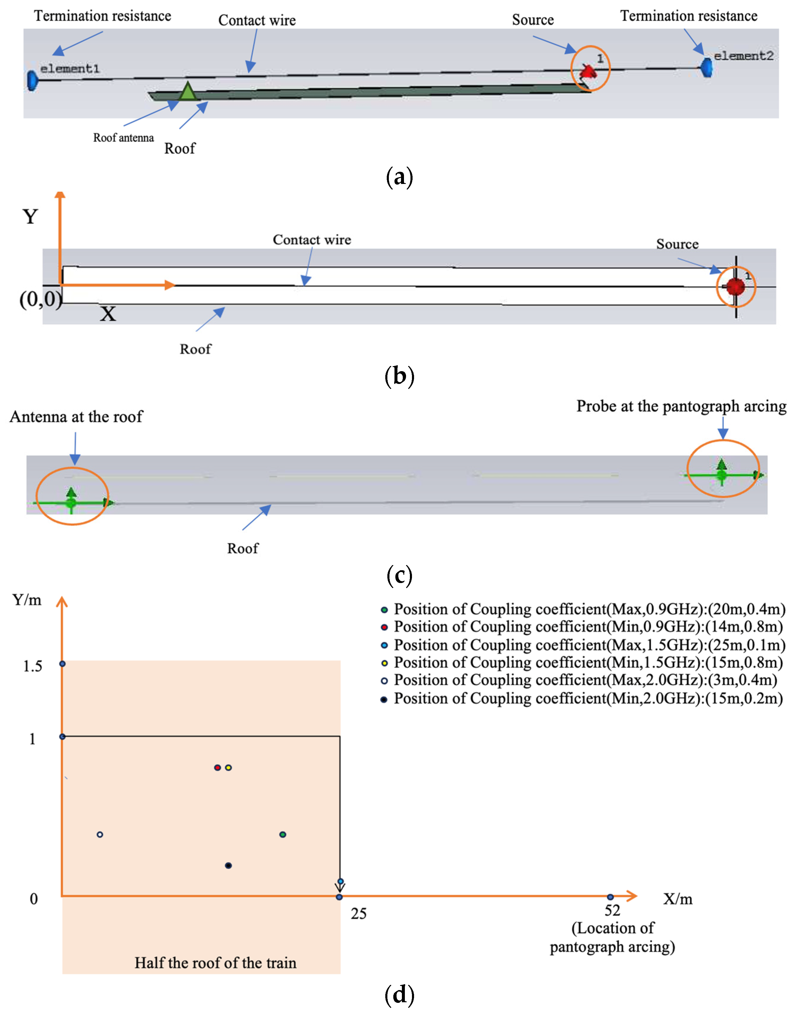
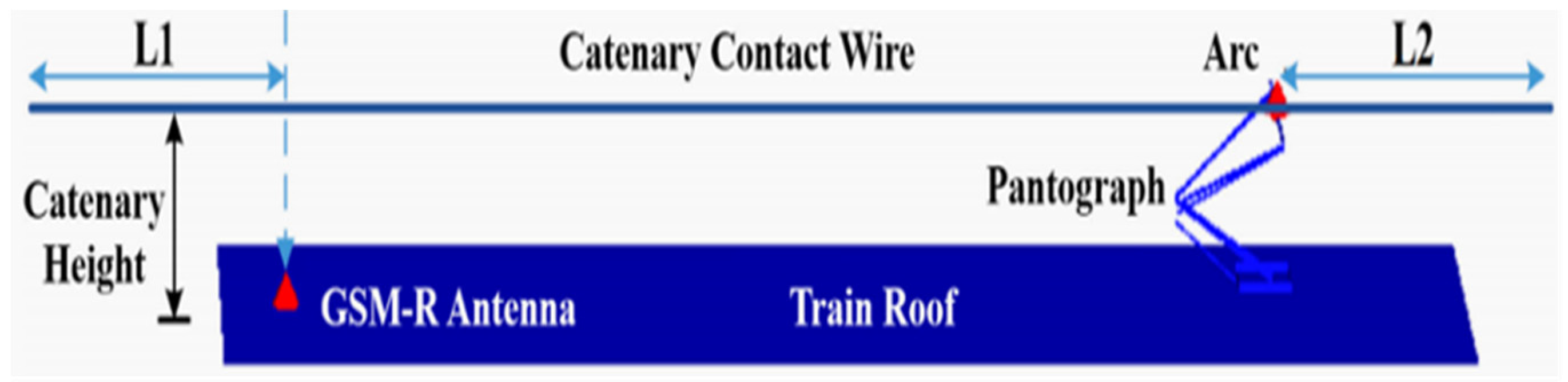
2. Coupling Coefficient Data
3. A Fast Prediction Model for the Coupling Coefficient
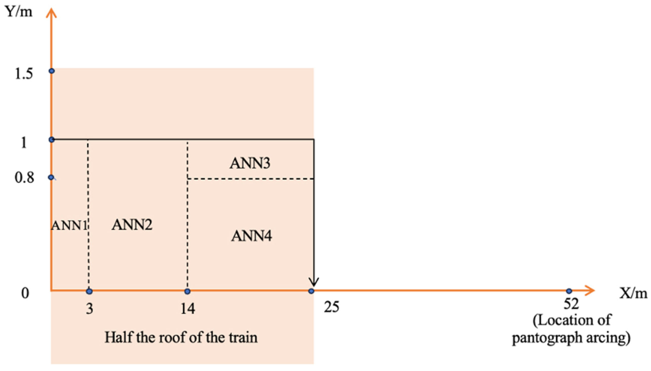
3.1. Setting of Prediction Model for the Coupling Coefficient

| Frequency (GHz) | Coupling Coefficient (Max) | Coupling Coefficient (Min) | Difference Value (dB) | ||
|---|---|---|---|---|---|
| Position (X, Y) (m) | Value (dB) | Position (X, Y) (m) | Value (dB) | ||
| 0.9 | 20, 0.4 | −50.10 | 14, 0.8 | −69.77 | 19.67 |
| 1.5 | 25, 0.1 | −52.75 | 15, 0.8 | −73.64 | 20.89 |
| 2.0 | 3, 0.4 | −30.4 | 15, 0.2 | −56.36 | 25.96 |
3.2. Structure of the MEA-BPNN
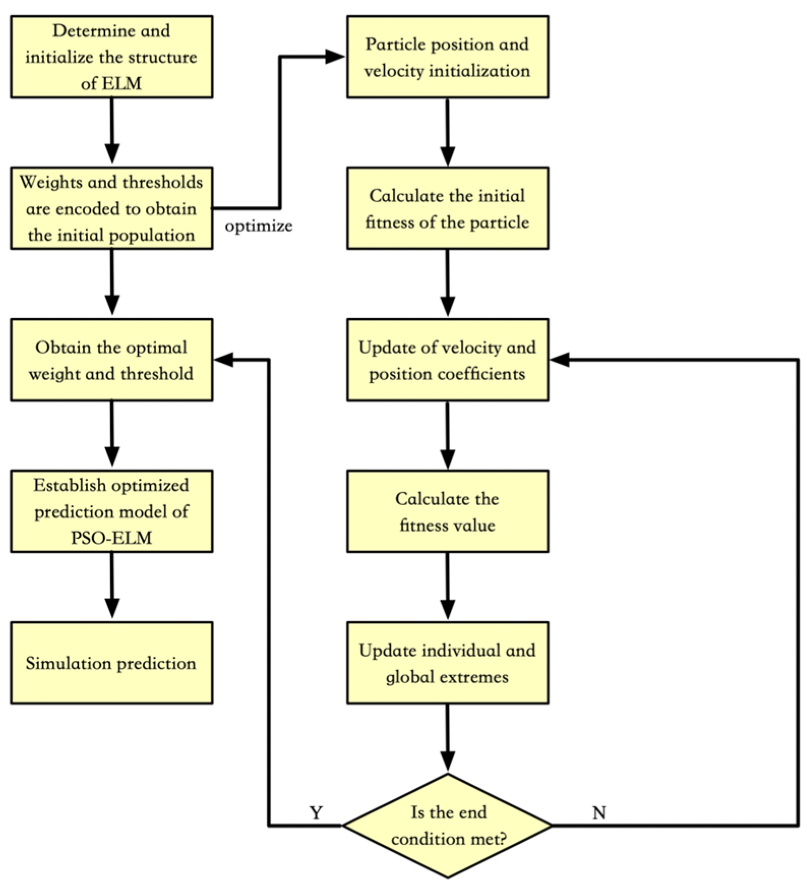
3.3. Structure of the PSO-ELM
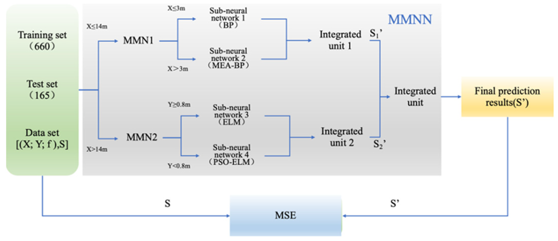
3.4. Structure of the MMNN
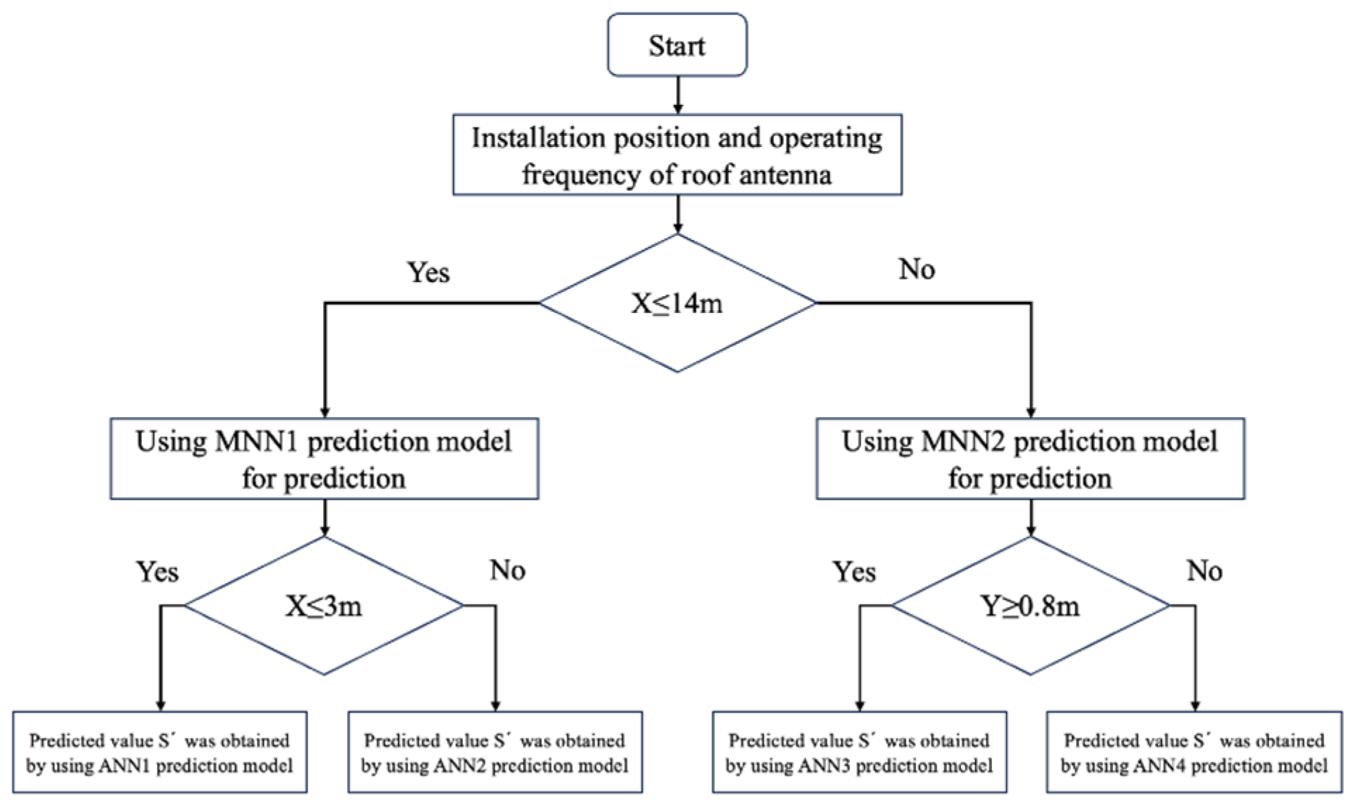
3.5. Prediction Model of Coupling Coefficient Based on MMNN
3.6. Prediction Results and Errors
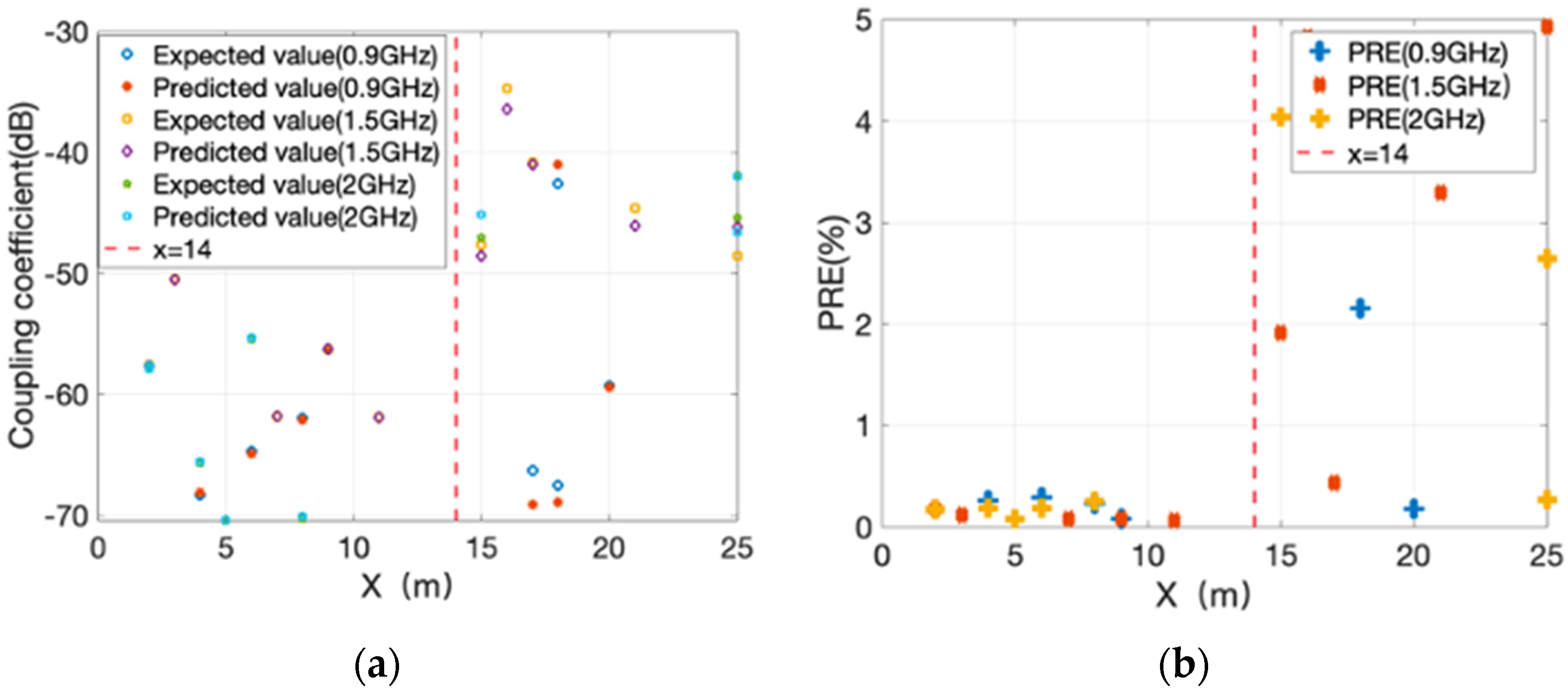
3.6.1. Prediction Results and Errors of MNN1 Prediction Model
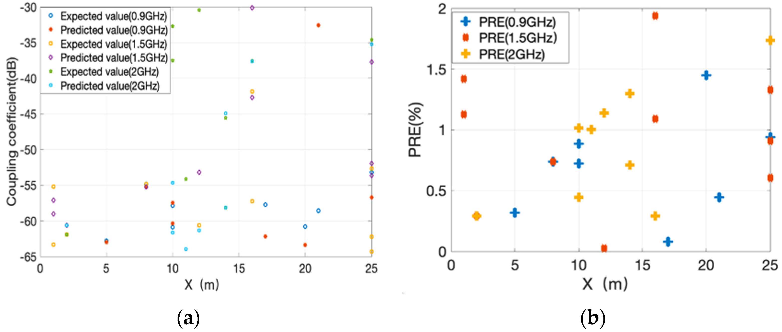
3.6.2. Prediction Results and Errors of MNN2 Prediction Model
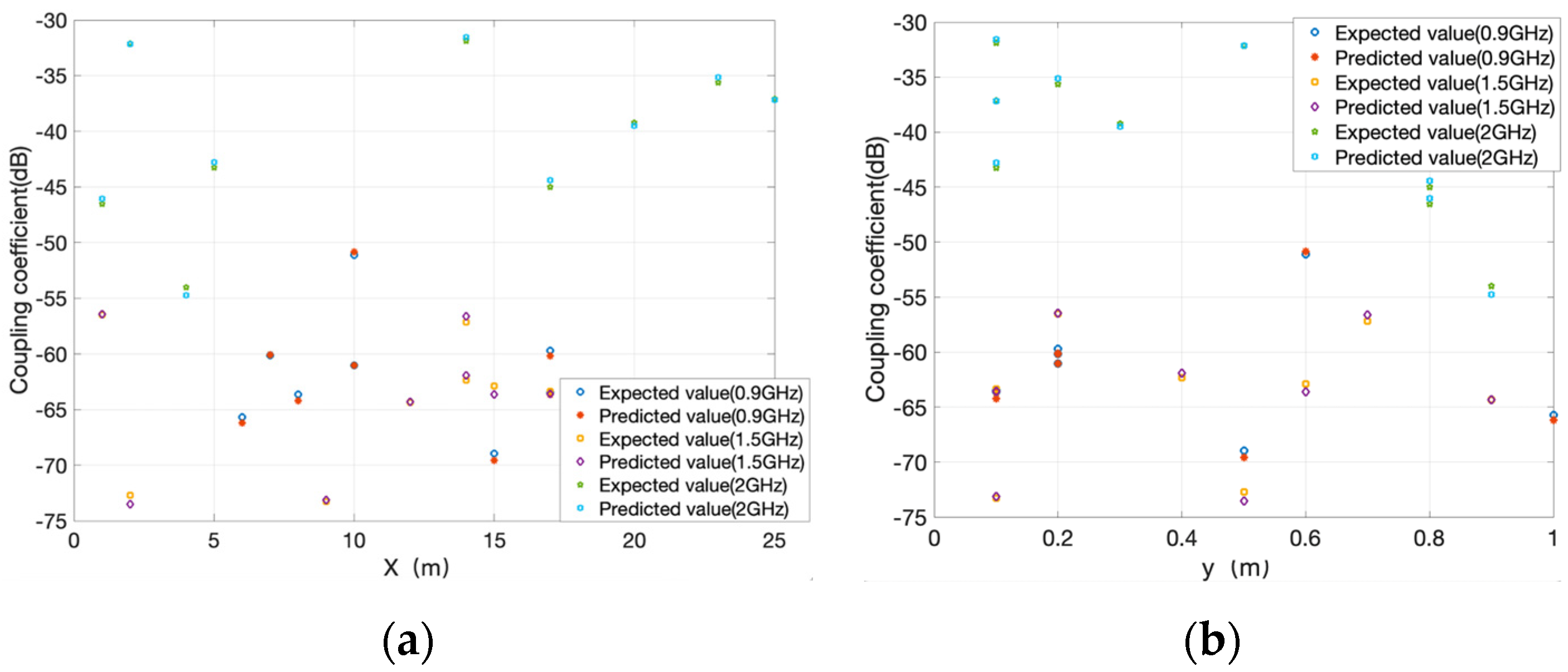
3.6.3. Prediction Results and Errors of Prediction Model Based on MMNN
4. Conclusions
Author Contributions
Funding
Institutional Review Board Statement
Informed Consent Statement
Data Availability Statement
Conflicts of Interest
References
- He, X.; Wen, Y.; Zhang, D. A Fast Prediction Method for the Electromagnetic Response of the LTE-R System Based on a PSO-BP Cascade Neural Network Model. Appl. Sci. 2023, 13, 6640. [Google Scholar] [CrossRef]
- Ma, L. The Radiated Characteristics of Pantograph Arcing in High-speed Railway. Ph.D. Thesis, Beijing Jiaotong University, Beijing, China, 2018. [Google Scholar]
- Mariscotti, A.; Marrese, A.; Pasquino, N. Time and frequency characterization of radiated disturbances in telecommunication bands due to pantograph arcing. In Proceedings of the Instrumentation & Measurement Technology Conference, Graz, Austria, 13–16 May 2012; pp. 2178–2182. [Google Scholar]
- Ma, L.; Wen, Y.; Marvin, A.; Karadimou, E.; Armstrong, R.; Cao, H. A Novel Method for Calculating the Radiated Disturbance from Pantograph Arcing in High-speed Railway. IEEE Trans. Veh. Technol. 2017, 66, 8734–8745. [Google Scholar] [CrossRef]
- Tang, Y. Research On Model Characteristics and EMI of Pantograph-Catenary Arc of the High Speed Train. Ph.D. Thesis, Southwest Jiaotong University, Chengdu, China, 2021. [Google Scholar]
- Wang, S. Research on Time Domain and Time Domain Propagation Characteristics of Electric Field Noise Radiated from Pantograph-Catenary Arc. Master’s Thesis, Liaoning Technical University, Fuxin, China, 2019. [Google Scholar]
- Shan, Q. Research on Key Techniques of Electromagnetic Compatibility for the China Railway High-Speed. Ph.D. Thesis, Beijing Jiaotong University, Beijing, China, 2013. [Google Scholar]
- Wang, J. The Influence of Pantograph Arcing Radiation Disturbance on Communication Quality of LTE-R. Master’s Thesis, Beijing Jiaotong University, Beijing, China, 2020. [Google Scholar]
- Zhang, S. Method for Predicting Electromagnetic Response of Sensitive Equipment Based on Neural Network. Master’s Thesis, Beijing Jiaotong University, Beijing, China, 2021. [Google Scholar]
- Ling, S. Research on Coverage Technologies of New Generation Wideband Railway Mobile Communications and Their Applications in Trial Systems. Ph.D. Thesis, Nanjing University of Posts and Telecommunications, Nanjing, China, 2022. [Google Scholar]
- Xu, H. Research on Key Technologies and Resource Allocation Algorithms of High Speed Railway Wireless Communication based on 5G. Ph.D. Thesis, China Academy of Railway Sciences, Beijing, China, 2022. [Google Scholar]
- Song, Y.; Wen, Y.; Zhang, D.; Lin, S.; Wang, W. Fast Prediction Model of Coupling Coefficient Between Pantograph Arcing and GSM-R Antenna. IEEE Trans. Veh. Technol. 2020, 69, 1612–11618. [Google Scholar] [CrossRef]
- Pu, S. Integrative Modelling and Analysis of Radio Frequency Link for Wireless Communication in Railway Environments. Ph.D. Thesis, Beijing University of Technology, Beijing, China, 2011. [Google Scholar]
- Li, D. Research on the Radio Coverage Characteristics in Confined Space. Ph.D. Thesis, Beijing University of Technology, Beijing, China, 2016. [Google Scholar]
- Dou, Y.; Li, Y.; Li, H.; Bao, J.; Lin, W. Isolation between Vehicle-Mounted Antennas for 350 km/h Chinese Standard EMU and Minimum Spacing. Chin. Railw. Sci. 2021, 42, 130–136. [Google Scholar]
- Dong, G.; Li, Y.; Li, H.; Bao, J.; Lin, W. Research on Performance and Interference Isolation of EMU’s Roof-mounted 450 MHz Frequency Band Antennas. Railw. Sign. Comm. 2021, 57, 42–47. [Google Scholar]
- Zhu, Q.; Chen, S. Shipboard Antennas Layout Based on Multi-Objective Optimization Algorithm. Sh. Sci. Technol. 2014, 36, 132–135. [Google Scholar]
- Song, Y.; Wen, Y.; Zhang, J.; Zhang, D. Fast Prediction Model for the Susceptibility of Balise Transmission Module System Based on Neural Network. In Proceedings of the 2019 International Conference on Electromagnetics in Advanced Applications, Granada, Spain, 9–13 September 2019; pp. 0445–0448. [Google Scholar]
- Wei, M. Research on Current Distribution and Control Strategy of Hybrid Excitation Synchronous Motor Speed Control System. Master’s Thesis, Xi‘an University of Technology, Xi’an, China, 2023. [Google Scholar]
- Zhang, W. Research on Fast Simulation Method of electromagnetic radiation of Arc between Pantograph and Catenary. Master’s Thesis, Liaoning Technical University, Fuxin, China, 2023. [Google Scholar]
- Wang, X. Analysis of 43 Cases of MATLAB Neural Networks, 1st ed.; Beihang University Press: Beijing, China, 2013; pp. 11–18. [Google Scholar]
- Sun, C.; Sun, Y.; Xie, K. Mind-evolution-based machine learning and applications. In Proceedings of the 3rd World Congress on Intelligent Control and Automation, Hefei, China; 2000; pp. 112–117. [Google Scholar]
- Wang, X.; Lin, Q.; Wu, H.; Zhao, P. Large Signal Modeling Method Based on MEA-BP Neural Network. In Proceedings of the International Conference on Microwave and Millimeter Wave Technology (ICMMT), Harbin, China, 12–15 August 2022; pp. 1–3. [Google Scholar]
- Zhu, Z.; Pang, Y.; Chen, Y. A Fault Diagnosis Method for Satellite Reaction Wheel Based on PSO-ELM. In Proceedings of the 2022 41st Chinese Control Conference (CCC), Hefei, China, 25–27 July 2022; pp. 4002–4007. [Google Scholar]
- Lu, C. Research on Design of Self-Organizing Modular Neural Network and Its Applications on Wastewater Detection. Ph.D. Thesis, Beijing University of Technology, Beijing, China, 2018. [Google Scholar]
- Song, Y. Research and Application on Electromagnetic Coupling of Vehicle Antenna of High-Speed Train Based on Artificial Intelligence. Ph.D. Thesis, Beijing Jiaotong University, Beijing, China, 2022. [Google Scholar]
- Zhang, Z. The Study Of Self-Organization Modular Neural Network Architecture Design. Ph.D. Thesis, Beijing University of Technology, Beijing, China, 2013. [Google Scholar]


| Installation Position (X, Y) (m) | Port of Monopole Antenna (1.268 GHz) | Port of Monopole Antenna (2 GHz) |
|---|---|---|
| (3, 0) | −43.52 dB | −50.21 dB |
| (5, 0) | −41.82 dB | −58.55 dB |
| (3, 0.5) | −49.27 dB | −63.46 dB |
| Position (X, Y) (m) | Frequency (GHz) | Coupling Coefficient (dB) |
|---|---|---|
| 1, 0 | 0.9 | −59.9 |
| 25, 0 | 0.9 | −65.4 |
| 24, 1 | 2.0 | −63.8 |
| 25, 1 | 2.0 | −53.7 |
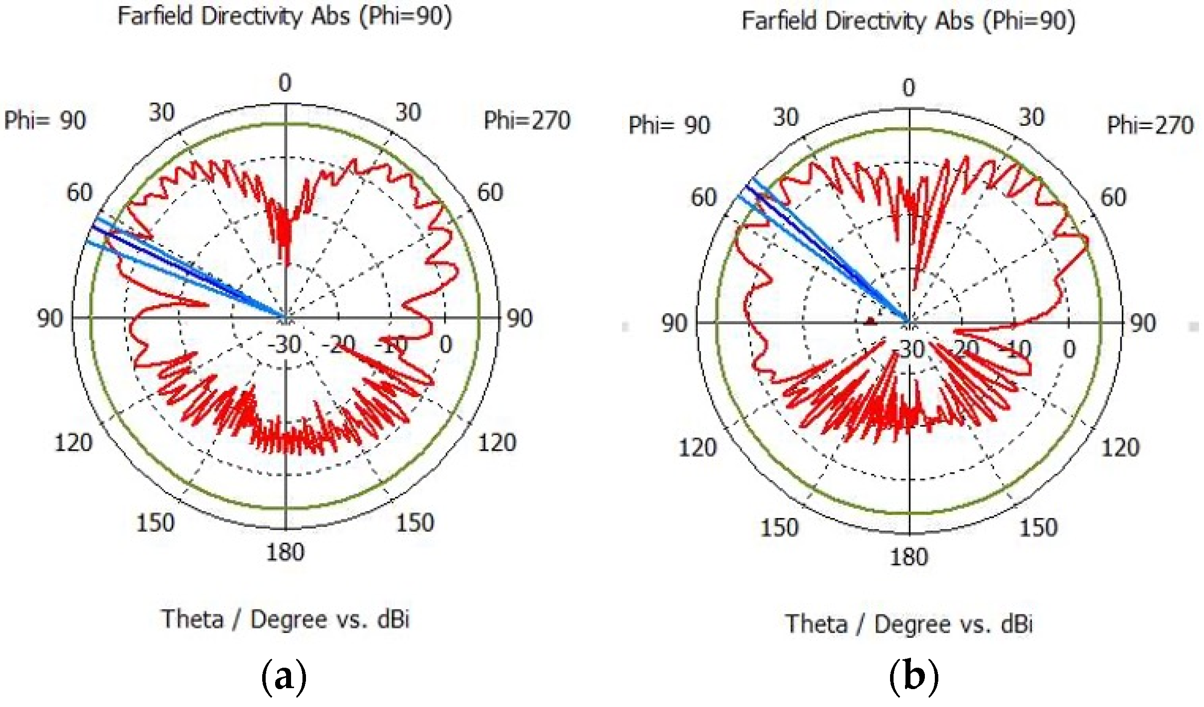
| Frequency (GHz) | Coupling Coefficient (Max) | Coupling Coefficient (Min) | ||||
|---|---|---|---|---|---|---|
| Position (X, Y) (m) | MLA (dBi) | MLD (°) | Position (X, Y) (m) | MLA (dBi) | MLD (°) | |
| 0.9 | 20, 0.4 | 4.96 | 71.0 | 14, 0.8 | 5.24 | 62.0 |
| 1.5 | 25, 0.1 | 4.98 | 61.0 | 15, 0.8 | 5.00 | 65.0 |
| 2.0 | 3, 0.4 | 6.81 | 65.0 | 15, 0.2 | 6.73 | 50.0 |
| X ≤ 3 m | 3 m < X ≤ 14 m | |||||
|---|---|---|---|---|---|---|
| MSE | MAE | PREMax | MSE | MAE | PREMax | |
| Sub-NN1 (BP) | 0.005 | 0.063 | 0.28% | 0.212 | 0.385 | 1.90% |
| Sub-NN2 (MEA-BP) | 0.005 | 0.055 | 0.31% | 0.006 | 0.066 | 0.33% |
| X ≤ 14 m | 14 m < X ≤ 25 m | |||||
|---|---|---|---|---|---|---|
| MSE | MAE | PREMax | MSE | MAE | PREMax | |
| MNN1 | 0.009 | 0.081 | 0.31% | 1.062 | 0.863 | 3.33% |
| Parameters | Value |
|---|---|
| Acceleration factor c1 | 2.49445 |
| Acceleration factor c2 | 2.49445 |
| Number of iterations | 200 |
| Maximum velocity | 1 |
| Minimum velocity | −1 |
| Maximum position | 5 |
| Minimum position | −5 |
| 0.8 m ≤ Y ≤ 1 m (14 m < X ≤ 25 m) | Y < 0.8 m (14 m < X ≤ 25 m) | |||||
|---|---|---|---|---|---|---|
| MSE | MAE | PREMax | MSE | MAE | PREMax | |
| Sub-NN3 (ELM) | 0.003 | 0.041 | 2.11% | 0.006 | 0.072 | 3.32% |
| Sub-NN4 (PSO-ELM) | 0.001 | 0.032 | 1.93% | 0.003 | 0.043 | 2.14% |
| X ≤ 14 m | 14 m < X ≤ 25 m | |||||
|---|---|---|---|---|---|---|
| MSE | MAE | PREMax | MSE | MAE | PREMax | |
| MNN2 | 0.361 | 0.511 | 1.95% | 0.438 | 0.557 | 2.12% |
| Frequency (GHz) | MSE | MAE | PREMax |
|---|---|---|---|
| 0.9 | 0.003 | 0.037 | 1.90% |
| 1.5 | 0.003 | 0.040 | 2.01% |
| 2.0 | 0.002 | 0.033 | 1.52% |
| Prediction Model | MSE | MAE | PREMax |
|---|---|---|---|
| MMNN | 0.002 | 0.033 | 1.52% |
| BP | 0.008 | 0.073 | 3.23% |
| MEA-BP | 0.004 | 0.056 | 2.51% |
| ELM | 0.005 | 0.060 | 3.06% |
| PSO-ELM | 0.004 | 0.058 | 2.35% |
| Computation Time | Storage Space | Coupling Coefficient (dB) | PRE | |
|---|---|---|---|---|
| Electromagnetic simulation | 41 min | 352 MB | −60.21 | 2.01% |
| Prediction model (MMNN) | 68 s | 3.2 MB | −61.42 |
Disclaimer/Publisher’s Note: The statements, opinions and data contained in all publications are solely those of the individual author(s) and contributor(s) and not of MDPI and/or the editor(s). MDPI and/or the editor(s) disclaim responsibility for any injury to people or property resulting from any ideas, methods, instructions or products referred to in the content. |
© 2024 by the authors. Licensee MDPI, Basel, Switzerland. This article is an open access article distributed under the terms and conditions of the Creative Commons Attribution (CC BY) license (https://creativecommons.org/licenses/by/4.0/).
Share and Cite
Bai, Y.; Ren, J.; Wen, Y. Fast Optimization of the Installation Position of 5G-R Antenna on the Train Roof. Appl. Sci. 2024, 14, 6954. https://doi.org/10.3390/app14166954
Bai Y, Ren J, Wen Y. Fast Optimization of the Installation Position of 5G-R Antenna on the Train Roof. Applied Sciences. 2024; 14(16):6954. https://doi.org/10.3390/app14166954
Chicago/Turabian StyleBai, Yu, Jie Ren, and Yinghong Wen. 2024. "Fast Optimization of the Installation Position of 5G-R Antenna on the Train Roof" Applied Sciences 14, no. 16: 6954. https://doi.org/10.3390/app14166954