Article

Fast Optimization of the Installation Position of 5G-R Antenna on the Train Roof

1
Institute of Electromagnetic Safety and Electromagnetic Protection, School of Automation and Intelligence, Beijing Jiaotong University, Beijing 100044, China
2
Frontiers Science Center for Smart High-Speed Railway System, Beijing Jiaotong University, Beijing 100044, China
*
Author to whom correspondence should be addressed.
Appl. Sci. 2024, 14(16), 6954; https://doi.org/10.3390/app14166954
Submission received: 17 June 2024 / Revised: 22 July 2024 / Accepted: 25 July 2024 / Published: 8 August 2024

Abstract

:
In this paper, a prediction model of the coupling coefficient based on a multi-module neural network (MMNN) is developed to quickly optimize the installation position of the roof antenna of the 5G-Railway (5G-R) communication system, so as to improve the anti-interference performance of the roof antenna. Firstly, a simulation model of the coupling coefficient between the pantograph arcing and the roof antenna (a monopole antenna operating frequency of 2 GHz) was established to construct the dataset. It is also verified that the influence of the electromagnetic interference (EMI) of pantograph arcing can be significantly reduced by predicting the new installation position (minimum coupling coefficient), and the installation position optimization of roof antenna can be realized. Then, the mind evolutionary algorithm of the back propagation neural network (MEA-BP) algorithm and particle swarm optimization—extreme learning machine (PSO-ELM) algorithm were adopted, respectively. The extreme learning machine algorithm constructed a different prediction model. And, by setting the integrated strategy of piecewise prediction, the prediction results are optimized and the accuracy of the prediction model based on the MMNN is further improved. Finally, the prediction model is proven to be able to replace the complicated electromagnetic simulation work accurately and efficiently by a variety of prediction performance indices, which provides an effective prediction method for the rapid optimization of the installation position of the roof antenna.

1. Introduction

The electromagnetic interference (EMI) protection of the on-board sensitive equipment of high-speed trains is the main basis for electromagnetic compatibility (EMC) design, and also the primary requirement to ensure the safe operation of trains [1]. The wireless communication systems such as Global System for Mobile Communications for Railway (GSM-R) and Long-Term Evolution for Railway (LTE-R) bear the responsibility of information transmission for train control, ensuring the safe operation of high-speed trains. The electromagnetic environment of the high-speed rail system is complex, and the roof antenna faces many sources of EMI, and the EMI caused by the inevitability and sudden pantograph arcing is one of the most common ones. Because of the wireless communication roof antenna and pantograph arcing located above the roof, and in order to ensure the communication quality, it is difficult to use shielding technology to improve the anti-interference performance of the roof antenna [2]. Based on previous research, the main power spectrum range of pantograph arcing is from a few hundred Hz to a few GHz [3]. It interferes with antenna reception and may cause communication anomalies. Ref. [4] learned, through experiments in a reverberation chamber, that the power range of the radiation electric field strength of the pantograph arcing coupled to the GSM-R antenna port is −58.6 dBm~−50.17 dBm, which is greater than the minimum received signal intensity of the on-board receiver (−95 dBm), which will cause EMI to the GSM-R receiver and endanger driving safety. According to the measured results, it is found that, with the increase in vehicle speed, the radiation field intensity of pantograph arcing at the same frequency will be significantly increased [5]. Therefore, with the increasing speed of high-speed trains in the future, the anti-interference research of the 5G-R antenna urgently needs to be carried out.
Much research has studied the impact of pantograph arcing on wireless communication transmission systems, especially the transmission quality of the GSM-R signal. For example, reference [6], based on the self-developed experimental device, carried out an experiment on the radiated electric field intensity of a single pantograph arcing in the anechoic chamber, and determined that the pantograph arcing would cause EMI to the GSM-R communication system. Based on the statistical analysis results of a large number of measured data, reference [7] studied the radiation electric field intensity of pantograph arcing, and finally obtained the amplitude probability distribution (APD) of EMI signals. Finally, the useful signal field strength required to ensure the bit error rate (BER) required by the communication system is analyzed. Refs. [8,9] simulated the downstream physical layer link of the LTE-R communication system by MATLAB, and concluded that the EMI caused by pantograph arcing would increase the block error ratio (BLER) of the LTE-R system (the operating frequency is 400 MHz). As a result, the number of instances of retransmission increases and the effective throughput of the system decreases by up to 21%, which seriously affects the communication quality of the system.
However, with the rapid development of railway intelligence and information technology, the needs of communication services between trains and the ground are constantly increasing. As a second-generation mobile communication technology, GSM-R fails to meet the large data communication requirements of video surveillance, video conferencing, passenger service, and other high-bandwidth applications on high-speed railways [10]. However, 5G has the technical characteristics of a large bandwidth, large connection, high reliability, and low delay, which not only supports the multi-priority service quality level guarantee, but also has the high-speed adaptability of 500 km/h, which is in line with the application scenario of high-speed rail [11]. It will be a trend for 5G to replace GSM in railway applications.
At present, there are few works of research on the calculation of the coupling coefficient and anti-interference measures between the pantograph arcing and 5G-R antenna. The EMI of the pantograph arcing is mainly coupled to the roof antenna port through radiation. Refs. [2,12] used electromagnetic simulation software to calculate the coupling coefficient between the pantograph arcing and the GSM-R antenna. Due to the relatively small impact of the body of the carriage on the EMI coupling pathway of the roof, the simulation model can be simplified to the case of only the roof, as shown in Figure 1. The coupling coefficient is defined as the radiation electric field intensity of the pantograph arcing coupled to the roof antenna, which can be calculated through simulation. The roof antenna in the simulation model is set as a quarter wavelength (λ/4) monopole antenna of 900 MHz, and the scaled model of the pantograph arcing and the roof antenna is built in the laboratory, and the coupling coefficient between the two is measured. By comparing the results of the simulation and laboratory measurement, it is shown that there is a small error (2.12 dB) between the two coupling coefficients, which proves the validity of the simulation model, and proves that the roof antenna can be set as a λ/4 monopole antenna. In addition, the commonly used car roof antenna is designed based on the basic structure of the λ/4 monopole antenna with an external antenna housing, such as the Katherin 741009 antenna, so the λ/4 monopole antenna is commonly used for simulation calculation [13,14].
In order to improve the anti-interference performance of the roof antenna, there are a lot of works of research on the optimization of the installation position of the roof antenna. Refs. [15,16] are based on the current deployment and future planning of the vehicle-mounted terminals in the Chinese standard electric multiple unit (EMU). Taking the GSM-R system of the 900 MHz band, and the LTE-R system of the 450 MHz band and 2.1 GHz band as examples, the stray interference of vehicle-mounted terminals is theoretically analyzed. Then, based on the theoretical model calculation of free space loss, the electromagnetic software simulation, and the measured results of the test platform, the isolation of roof antennae is studied and a reasonable antenna spacing is proposed to meet the needs of the interference isolation of vehicle-mounted communication terminals. The installation position of the roof antenna can be further optimized by using various intelligent optimization algorithms. Ref. [17] proposed an antenna optimization layout method based on the multi-objective particle swarm optimization (MOPSO) algorithm to address the shortcomings of existing single-objective optimization algorithms in the antenna layout. The algorithm is combined with the numerical calculation method, and the effectiveness of the proposed method is verified by placing three short-wave communication antennae on the ship simulation model.
The above references point out the importance of studying the installation position of roof antennae, and provide the research basis for the installation of roof antennae or ship-borne antennae by using the traditional electromagnetic simulation method. However, the research purpose of the above references is to reduce the electromagnetic coupling degree between antennae, and the EMI caused by pantograph arcing is not included in the study of the optimization of the installation position of the 5G-R antenna.
In summary, in order to further optimize the installation position of the roof antenna, it is necessary to focus on the EMI of the pantograph arcing on the 5G-R antenna. In addition, in view of the large roof plane (length × width of about 25 m × 3 m), and referring to the “Fuxing” train of 17 groups, the distance between the roof antenna and the pantograph arcing can reach up to two carriages (about 50 m). Therefore, when using electromagnetic simulation methods for research, new methods are urgently needed to replace a large number of repeated simulations and multi-parameter effects, so as to effectively replace the complicated electromagnetic simulation work. When using the electromagnetic simulation method to study and analyze the installation position of the roof antenna, the most important step is to accurately model the roof and the antenna. However, due to the large roof area and the variable installation position of the roof antenna, such complicated simulation work will consume a lot of time and occupy a large amount of computer storage space, and, finally, will seriously affect the efficiency of research and analysis.
As more practical simulation parameters are applied in the future, such as roof obstacles, material parameters, and the influence of the surrounding environment, the shortcomings of this electromagnetic simulation method will become increasingly prominent. In recent years, with the continuous development of algorithms such as machine learning (ML) and deep learning (DL) in artificial intelligence (AI), many scientific research problems have been successfully solved. When ML algorithms are used to solve electromagnetic problems, the number of repeated electromagnetic simulations and the occupied storage space will be greatly reduced. For example, a fast prediction model for the electromagnetic sensitivity of the balise transmission module (BTM) system based on a BP neural network (BPNN) algorithm is established in [18]. BPNNs have the advantage of being computationally simple and easy to use, but they also have the obvious disadvantage where the network training is prone to become stuck in local minima and the learning process converges slowly. In order to solve this problem, other algorithms can be used to replace or combine the global optimization algorithm and BP algorithm, such as the ELM algorithm or MEA-BP algorithm.
Both the MEA-BPNN algorithm and ELM algorithm can be used to predict EMC problems. The MEA-BPNN algorithm was used to establish a current distribution prediction controller, which significantly reduced the phenomenon of various current components of the motor when the inductance parameters were mismatched [19]. The ELM algorithm was applied to establish a fast prediction model for the radiation field of pantograph arcing, and, finally, the validity and accuracy of the prediction model was verified [20].
A coupling coefficient prediction model based on the multi-module neural network (MMNN) is proposed in this paper. Firstly, a simulation model of the coupling coefficient between the pantograph arcing and the roof antenna (a monopole antenna operating frequency of 2 GHz) was established to construct the dataset. It is also verified that the new installation position (the lowest coupling coefficient) can significantly reduce the influence of EMI caused by pantograph arcing, so as to optimize the installation position of the roof antenna. Then, on the basis of the preliminary analysis of the data change rule, the sub-module prediction model is established by the MEA-BP algorithm and the PSO-ELM algorithm, respectively. By setting the integrated strategy of piecewise prediction, the prediction results are optimized and the accuracy of the prediction model based on the MMNN is further improved. Finally, the prediction model is proven to be able to replace the complicated electromagnetic simulation work accurately and efficiently by a variety of prediction performance indices, which provides an effective prediction method for the rapid optimization of the installation position of the roof antenna.
The rest of this paper consists of three sections. In Section 2, data on the coupling coefficients are collected and analyzed. In Section 3, a prediction model of the coupling coefficient based on the MMNN is constructed and its accuracy and efficiency are verified. Finally, the conclusion is given in Section 4.

2. Coupling Coefficient Data

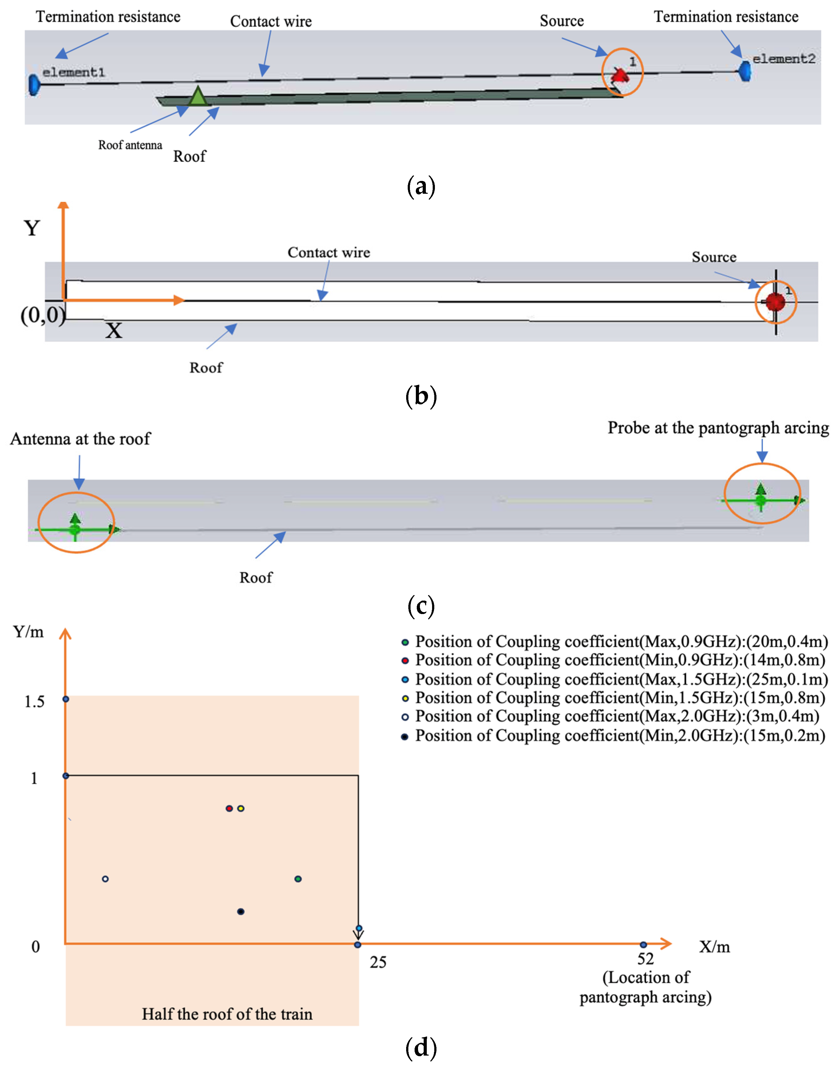
In order to quickly optimize the installation position of the 5G-R antenna, the coupling coefficient between the pantograph arcing and the roof antenna needs to be collected and analyzed. In this paper, the similar electromagnetic simulation model in references [2,12] is used to solve the coupling coefficient. Firstly, the simulation model of the coupling coefficient is established by using electromagnetic simulation software. As mentioned above, due to the limitation of the scale and simulation time of the electromagnetic simulation, the model can be simplified to only the case of the roof. The main view and top view of the model are shown in Figure 2.
In the model, the roof plane of a carriage is set to be 25 m × 3 m, given that the pantograph of the “Fuxing” train of 17 groups is located in the No. 3 and No. 6 carriages, and the roof antenna of the communication system is mostly located on the top of the first carriage. Therefore, the roof plane in the model is 50 m × 3 m, and the co-ordinate system marked in the figure is taken as a reference. The position co-ordinate of the pantograph arcing is (52 m, 0 m), and the roof antenna is located directly below the contact line, and the distance from the roof plane is 3 cm. A thin cylinder with a length of 3 cm is used to simulate the pantograph arcing. A voltage source with an amplitude of 1 kV is set at the center of the thin cylinder as the excitation source port, which is a discrete port. The contact wire is a finite length wire; in order to reduce the influence of the contact wire length on the coupling coefficient, it is necessary to connect the termination resistance at two terminals of the contact line [4]. The length of the contact line in reference [4] is 43 m, and the terminal resistance is set at 200 Ω. The length of the contact line in the simulation model in this paper is 80 m, so the terminal resistance is set at 250 Ω. In this paper, probes (with an interval of 1 cm) are set, respectively, near the pantograph arcing and above the roof antenna to collect the electric field intensity E1 and E2 at the two places, in units of dBV/m, as shown in Figure 2c. Therefore, in this paper, the coupling coefficient is defined as the difference between the two (S = E2 − E1); the unit is dB, which is used to determine the best installation position of the roof antenna with different operating frequencies, that is, the minimum value of the coupling coefficient [1]. The optimization of the installation position of the roof antenna is influenced by many factors, such as the electromagnetic coupling between the roof antennae, the distribution of electromagnetic field intensity in the roof area, and the installation height or size of the antenna.
Figure 2. A simplified model for the coupling coefficient of pantograph arcing and roof antenna: (a) front view of model; (b) top view of model; (c) probes of electric field simulation; and (d) installation position of antennae for Table 3.
Applsci 14 06954 g002
Among them, the study on the distribution of the radiant electric field intensity on the roof is too general, and can only obtain the change curve of the electric field intensity, failing to take into account the research objectives such as the working frequency and specific position of the roof antenna. In addition, if the parameters are changed, a large number of simulation solutions will be required and the calculation cost will be large. The electromagnetic coupling between the roof antennae and the installation height or size of the antenna need to be studied according to the specific model and the situation of the roof antenna, which is not considered in this paper.
Therefore, this paper focuses on the effect of the position co-ordinates (X, Y) of the 5G-R antenna on the coupling coefficient.
In this paper, a one-quarter wavelength monopole antenna with an operating frequency of 2 GHz (the main operating frequency of the 5G-R antenna) is used as the roof antenna for simulation, and the single simulation time is about 40 min. The simulation model established in this paper is based on the electromagnetic simulation software CST 2019. The numerical calculation method is using a time-domain solver, in which the mesh type is set to Hexahdral, the accuracy is set to −40 dB, and the adaptive mesh optimization function is used. The simulation computing platform used in this paper is an Intel®I7 12600KF® CPU with a WIN10 64-bit processing system and 16 GB of memory.
In order to further prove the validity of the simulation model, the coupling coefficient of the monopole antenna (operating frequency of 1.268 GHz), calculated by using the similar simulation model in reference [12], was compared. As shown in Table 1, the change rules of the two coupling coefficients are the same; that is, as the linear distance between the roof antenna and the pantograph arcing increases, the coupling coefficient naturally decreases, which is caused by the attenuation of electromagnetic wave propagation in free space.
However, since the roof in the simulation model of reference [12] is only 22 m × 2.82 m, the spacing between the roof antenna and the pantograph arcing under the same co-ordinates is smaller. In addition, the lower working frequency of the antenna and the different material settings in the simulation model will cause the inconsistency between the two coupling coefficients, but it is enough to prove that the simulation model in this paper can effectively construct the original dataset of coupling coefficients. When constructing the dataset, considering the actual installation requirements of the roof antenna and the size of the antenna, the distance of the horizontal co-ordinate X was increased from 1 m to 25 m at an interval of 1 m, and the distance of the vertical co-ordinate Y was increased from 0 m to 1 m at an equal interval of 0.1 m, so that a total of 275 co-ordinates were included.
In order to further verify the generalization of the prediction model in this paper, the coupling coefficients of two roof monopole antennae for the GSM-R system and the satellite navigation system are simulated at the same time, and their working frequencies are 0.9 GHz and 1.5 GHz, respectively. Therefore, 825 sets of different coupling coefficients can be obtained, and 80% of the data (660 sets) are randomly sampled as the training set, and the remaining 165 sets of data are used as the test set. Part of the simulation data (four sets) is shown in Table 2.

3. A Fast Prediction Model for the Coupling Coefficient

3.1. Setting of Prediction Model for the Coupling Coefficient

Table 3 shows the maximum coupling coefficients of three kinds of roof antennae and their corresponding installation positions, which are drawn as a schematic diagram, as shown in Figure 2d.
Table 3. Comparison of coupling coefficients of roof antennae with different frequencies.
Frequency (GHz)Coupling Coefficient (Max)Coupling Coefficient (Min)Difference Value (dB)
Position (X, Y) (m)Value (dB)Position (X, Y) (m)Value (dB)
0.920, 0.4−50.1014, 0.8−69.7719.67
1.525, 0.1−52.7515, 0.8−73.6420.89
2.03, 0.4−30.415, 0.2−56.3625.96
As can be seen from Table 3, when the operating frequency of the roof antenna is 2 GHz and the coupling coefficient reaches the maximum and minimum values, the installation co-ordinates of the roof antenna are (3, 0.4) and (15, 0.2), which are similar to the attenuation characteristics of the radiation field of the pantograph arcing; that is, the attenuation of the electric field intensity is small at the place far from the pantograph arcing. This is because the electric field strength here is mainly the result of the superposition of the radiation of the contact line and the reflection of the roof [2].
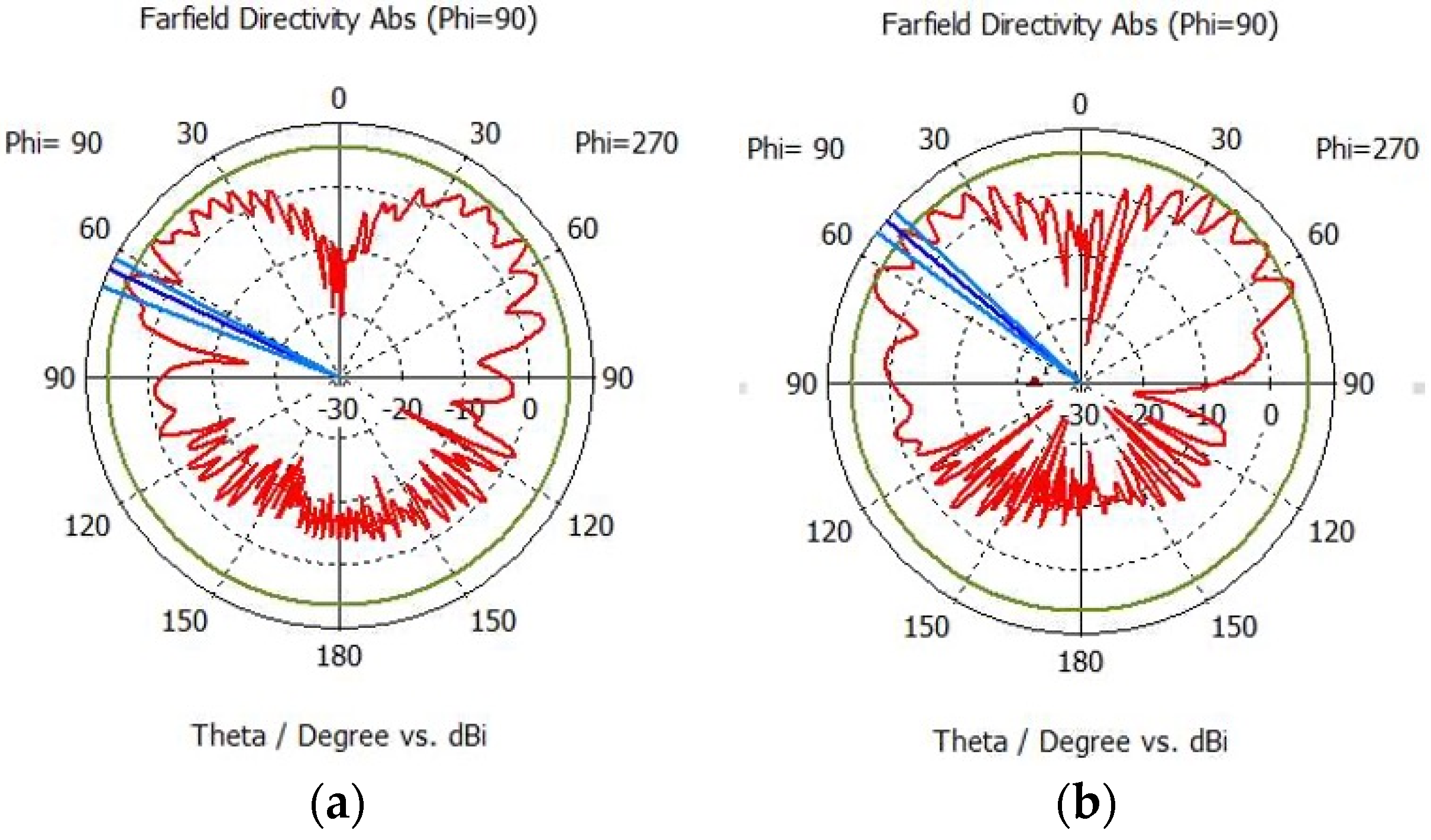
The performance of the antenna is greatly affected by the surrounding environment. Due to the influence of the roof metal plane reflection, the antenna pattern of the roof antenna will change greatly compared with that in free space. In addition, with different installation positions of the roof antenna, the antenna pattern and performance parameters (such as the main lobe magnitude and the main lobe direction) will also change [16]. Figure 3 shows the antenna pattern of the roof antenna at two installation positions (coupling coefficient(Max) and coupling coefficient(Min)) before and after optimization. Due to space limitations, only the antenna pattern of the roof antenna (f = 2 GHz) is displayed. Table 4 shows two antenna performance parameters (the main lobe magnitude (MLM) and main lobe direction (MLD) at six installation positions.
From Figure 3, it can be seen that, due to the reflection of the roof plane, the antenna pattern of the roof antenna (f = 2 GHz) is no longer symmetrical, but the shapes of the antenna patterns at the two installation positions are generally similar and have no significant changes. In addition, it can also be seen from Table 4 that the optimization of the installation position of the roof antenna with different operating frequencies has a small impact on the performances of the antenna. For the roof antenna (f = 2 GHz), the change in MLA is only 0.08 dbi, and MLD is reduced by 15°, so the optimization of the installation position does not significantly affect the performances of the roof antenna.
However, because of the difference in operating frequency, the two co-ordinates are also significantly different. This is due to the irregular phenomenon caused by the size of the roof antenna and other factors, so it is difficult to use the method of fitting the curve to predict. In addition, due to the irregular reflection of the roof plane and other environmental factors in practical applications, it is possible to affect the irregular variation of the attenuation characteristics of the radiant electric field intensity on the roof, so it is necessary to establish a more accurate prediction method for the coupling coefficient. However, it can still be seen from Table 3 that, among the 825 different positions in the dataset, the coupling coefficient can be reduced by up to 26.96 dB by optimizing the installation position of the roof antenna.
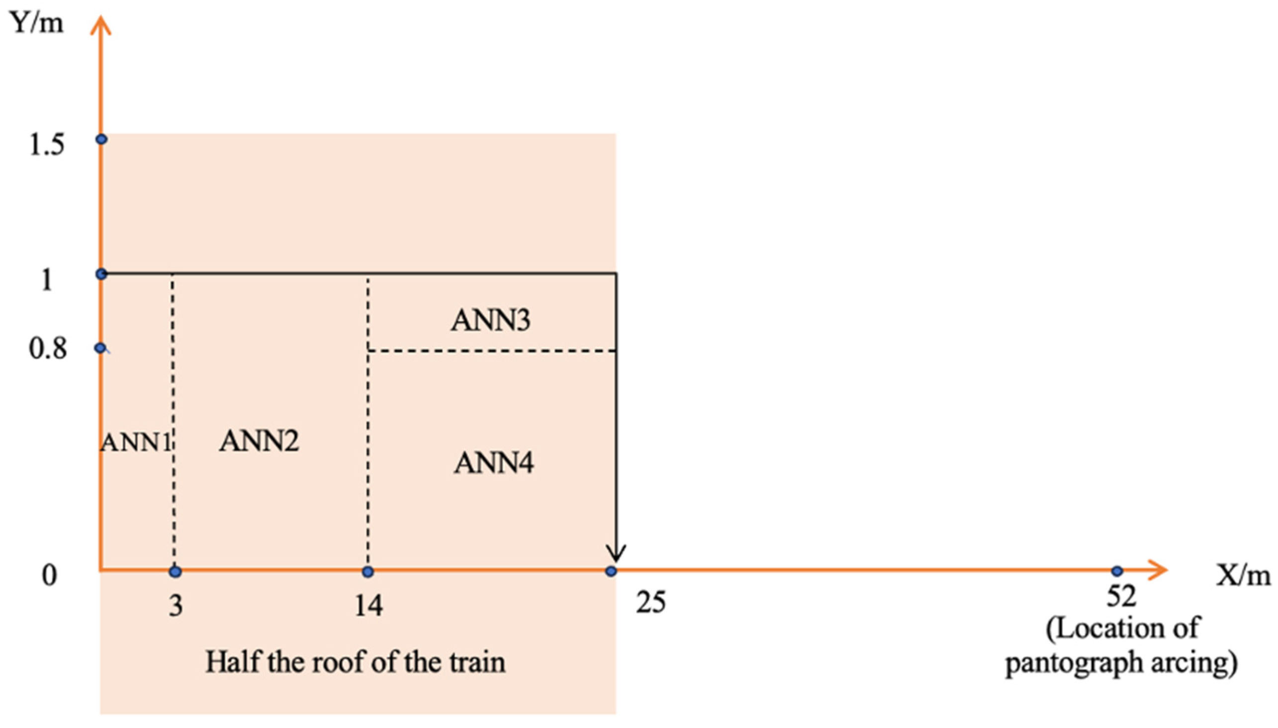
Therefore, if the installation position of the roof antenna with the lowest coupling coefficient can be found, the EMI of pantograph arcing can be significantly reduced. Methods based on prediction model to obtain such locations will be more efficient than methods based on multiple electromagnetic simulations or methods based on engineering experience. As mentioned above, this paper will build a prediction model based on the BPNN algorithm and ELM algorithm, optimize it with the MEA and PSO algorithm, and propose a prediction model based on the MMNN. Block modeling was carried out according to the roof plane in the model, as shown in Figure 4.
In reality, the contact line is generally located at the center line of the roof plane, that is, the X-axis in the figure, and the roof plane is symmetrically distributed accordingly, so only half of the roof plane area is considered in this paper.
As can be seen from Figure 4, in the range of the roof antenna installation currently considered, the roof plane is divided into four modules, with X as 3 m and 14 m, and Y as 0.8 m as the dividing lines, respectively, and four different algorithms are used for block modeling. Finally, the coupling coefficient of the roof antenna at different installation positions is predicted efficiently based on the prediction model. The selection of the three dividing lines is based on the comparison of the prediction accuracy of different single-prediction models, and gives full play to their respective strengths as much as possible. The analysis of the results will be presented later.
The accuracy of the BPNN prediction model and ELM prediction model is mainly affected by the parameters (weights and thresholds) between the neuron nodes of each layer in the structure, and these parameters are generated randomly, which may lead to a low prediction accuracy and instability [21].
To solve the above problems, the MEA and PSO algorithms are widely used to optimize the initial parameters, so that the prediction accuracy and stability of the prediction model have been significantly improved. Therefore, the MEA-BPNN prediction model and PSO-ELM prediction model will be constructed in this paper to predict the coupling coefficient of the roof antenna at different installation positions.

3.2. Structure of the MEA-BPNN

The BPNN is a one-way propagation feedforward neural network, which belongs to supervised learning algorithm and has a good nonlinear mapping ability. However, the optimal selection of weights and thresholds has not been solved theoretically. Generally, it is initialized as a random number between [−0.5, 0.5], but it will cause instability in the prediction accuracy, and there is still a large room for improvement as a prediction model. Aiming at the shortcomings of the genetic algorithm (GA) and other evolutionary algorithms such as the slow convergence speed, Sun proposed the MEA in 1998 [21,22]. As an optimization algorithm with a stronger optimization ability, the MEA follows the basic concepts of the GA such as “group” and “individual” and replaces “crossover” and “variation” with “convergence” and “dissimilation”. The former provides a parallel search ability and improves the optimization efficiency. The latter constantly updates the current optima to avoid falling into local optima; that is, it is responsible for local and global optimization, respectively, and the two are alternately carried out until the global optima is reached. Li established the MEA-BPNN prediction model, whose accuracy and stability are higher than the BPNN and GA-BPNN prediction model. For more detailed algorithms and steps, see reference [21,23]. In summary, the specific flow diagram of the MEA-BPNN prediction model algorithm is shown in Figure 5.

3.3. Structure of the PSO-ELM

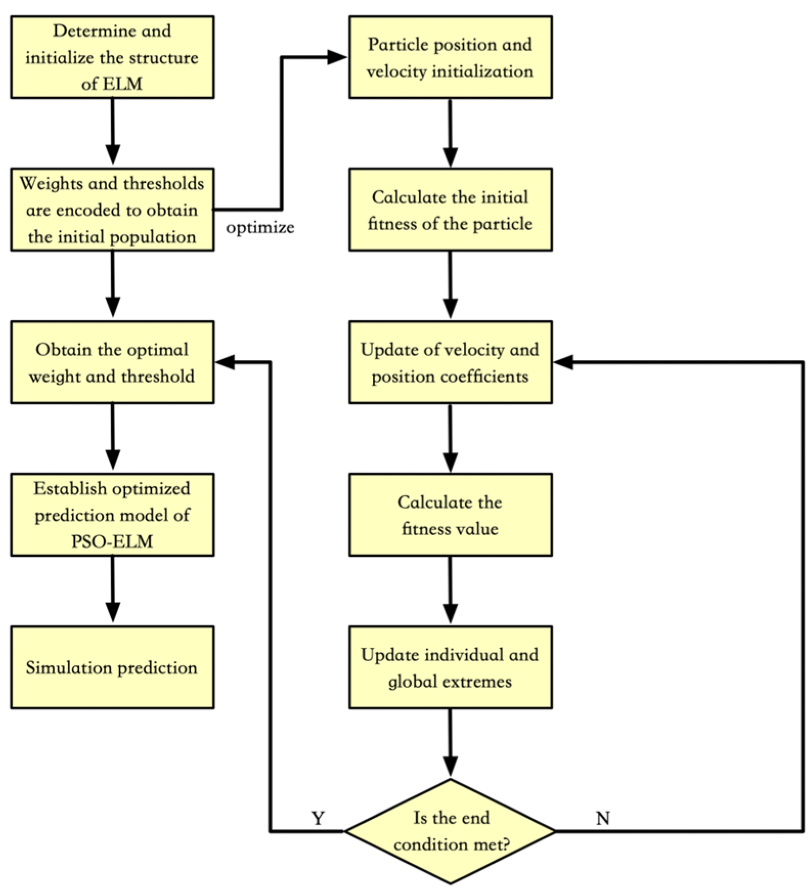
As mentioned above, improvements to the BPNN algorithm can also be made using alternative algorithms. Therefore, this paper applies the ELM algorithm, which can obtain the unique optimal solution only by setting the number of neuron nodes of the HL. It has the advantages of a simple structure, fast training speed, and strong generalization performance. But, during operation, the parameters (weights and thresholds) of the input layer (IL) and the HL will also be randomly generated. For more detailed algorithms and steps, see reference [21]. However, since these parameters are generated randomly, it may lead to the situation where the value is 0 when the parameters are given, which makes the output matrix unsatisfactory and there are many invalid neuron nodes, resulting in a poor accuracy and stability of prediction in the face of complex and irregular data. Therefore, the PSO algorithm can be used to optimize the initial parameters in the model in order to improve the accuracy and stability. When the PSO algorithm is used to train the ELM network, the weights and thresholds of neuron nodes in the structure are encoded into a particle swarm. The fitness value is the mean squared error (MSE) of the network output. First, the weight and threshold vector were initialized, and then the PSO algorithm is used to search for the optimal result; that is, the weights of the neuron nodes are searched within a defined number of iterations to minimize the output mean squared error of the network structure. The specific algorithm of the PSO algorithm can be referred to in reference [24]. The specific flow block diagram of the PSO-ELM algorithm is shown in Figure 6.

3.4. Structure of the MMNN

When dealing with complex practical problems, the prediction accuracy and generalization ability of the single-structure NN model may be poor, and it is difficult to meet the performance requirements of prediction. In order to further optimize the equivalent modeling analysis of complex problems, many scholars have introduced the concept of “multi-module and multi-task” into the structural design of the NN based on the fact of human brain task decomposition and functional partitioning, hoping to learn from this information processing mode and improve the performance of the NN prediction model [25]. The MMNN method decomposes complex practical problems into several combinations of multiple sub-neural network modules, each of which is independent and interrelated, and decomposes complex tasks into multiple different sub-tasks through the decomposition method. On the basis of processing different sub-tasks, the sub-network model finally improves the prediction accuracy through task integration [26,27]. The decomposition method of the MMNN and the principle and function of each sub-module can be referred to in reference [27].

3.5. Prediction Model of Coupling Coefficient Based on MMNN

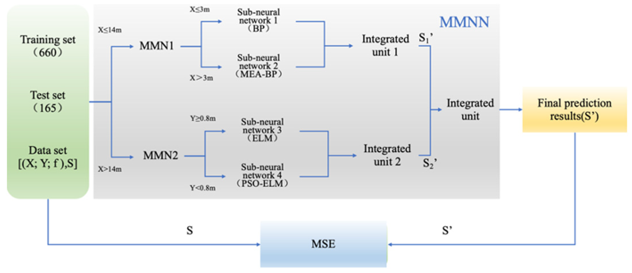
As mentioned above, this paper uses the MEA-BPNN algorithm and the PSO-ELM algorithm to construct sub-prediction models. Next, the prediction performance of the two prediction models before and after optimization is analyzed, and the prediction model based on the MMNN is finally established, as shown in Figure 7.
As shown in Figure 7, in the prediction model proposed in this paper, X = 14 m is first taken as the dividing line. When X ≤ 14 m, module neural network 1 (MMN1) is used for prediction; when X > 14 m, MNN2 is used for prediction. Then, in MNN1, with X = 3 m as the dividing line, a prediction model is constructed based on the BPNN algorithm and the MEA-BPNN algorithm, respectively, at X ≤ 3 m and X > 3 m, as sub-neural network 1 and sub-neural network 2, and then MNN1 is constructed by integrating strategies. Similarly, in MNN2, Y = 0.8 m is taken as the dividing line. When Y ≥ 0.8 m and Y < 0.8 m, prediction models based on the ELM algorithm and the PSO-ELM algorithm are constructed, respectively, as sub-neural networks 3 and sub-neural networks 4, and then MNN2 is constructed by integrating strategies. Finally, by integrating the predicted results of MNN1 and MNN2, the final predicted value is obtained.
In Figure 7, S represents the expected value of the coupling coefficient, and S 1 and S 2 represent the predicted values obtained from MNN1 and MNN2, respectively. In this paper, the MSE is used, as shown in Equation (1):
M S E = i = 1 N S i S i 2 N
where N represents the number of coupling coefficients, and S i   and S i represent the predicted values and expected values of the coupling coefficients corresponding to the roof antenna located at the i-th position, respectively. The MSE value is used to determine whether the established prediction model meets the preset accuracy requirements, which represents the accuracy of the prediction results. The smaller the value is, the more accurate the prediction results are, and the default target value is 0. When the MSE value is small enough, the accuracy requirements of the prediction model will be considered, and the training will stop, thus completing the construction of the prediction model [12].

3.6. Prediction Results and Errors

3.6.1. Prediction Results and Errors of MNN1 Prediction Model

In this paper, the MSE, mean absolute error (MAE), and relative prediction error (PRE) are used to judge the prediction accuracy. The MAE and PRE are shown in Equations (2) and (3), respectively. The MAE represents the consistency of the prediction results, and the smaller the value, the smaller the prediction deviation:
M A E = i = 1 N S i S i N
P R E = S i S i S i × 100 %
where N represents the number of coupling coefficients, and S i a n d   S i represent the predicted value and expected value of the coupling coefficient of the port when the roof antenna is located at the i-th position, respectively.
In order to meet the inherent needs of the prediction model, the input and output data should be normalized and anti-normalized; that is, before running the prediction model, the data should be normalized within the range of [0, 1]. The number of neurons in the hidden layer (HL) of the BPNN model was determined by the trial-and-error method. The calculation results showed that, when the number of neurons was 3, the prediction error was small. Therefore, the topology of the BPNN is 3-3-1, and the transfer functions of the HL and OL adopt the Tansig function and Purelin function, respectively. The maximum training times are 200, the minimum error of the training target is 0.0001, and the learning rate is 0.1. The size of the MEA population was 200, the number of subpopulations was 20, the number of superior subpopulations and temporary subpopulations were both 5, and the number of iterations was 10. In addition, in order to improve the reliability of the prediction results, all prediction models in this paper will be simulated for 10 consecutive times, and the average value of the 10 prediction results will be taken as the final result, as shown in Table 5.
As can be seen from Table 5, when X ≤ 3 m, the PERMax of sub-neural network 1 (Sub-NN1) and sub-neural network 2 (Sub-NN2) is 0.28% and 0.31%, respectively, and the other two performance indices are similar. However, sub-neural network 1 does not need to apply the MEA, and the structure of the prediction model is simpler, so the engineering practicability is better.
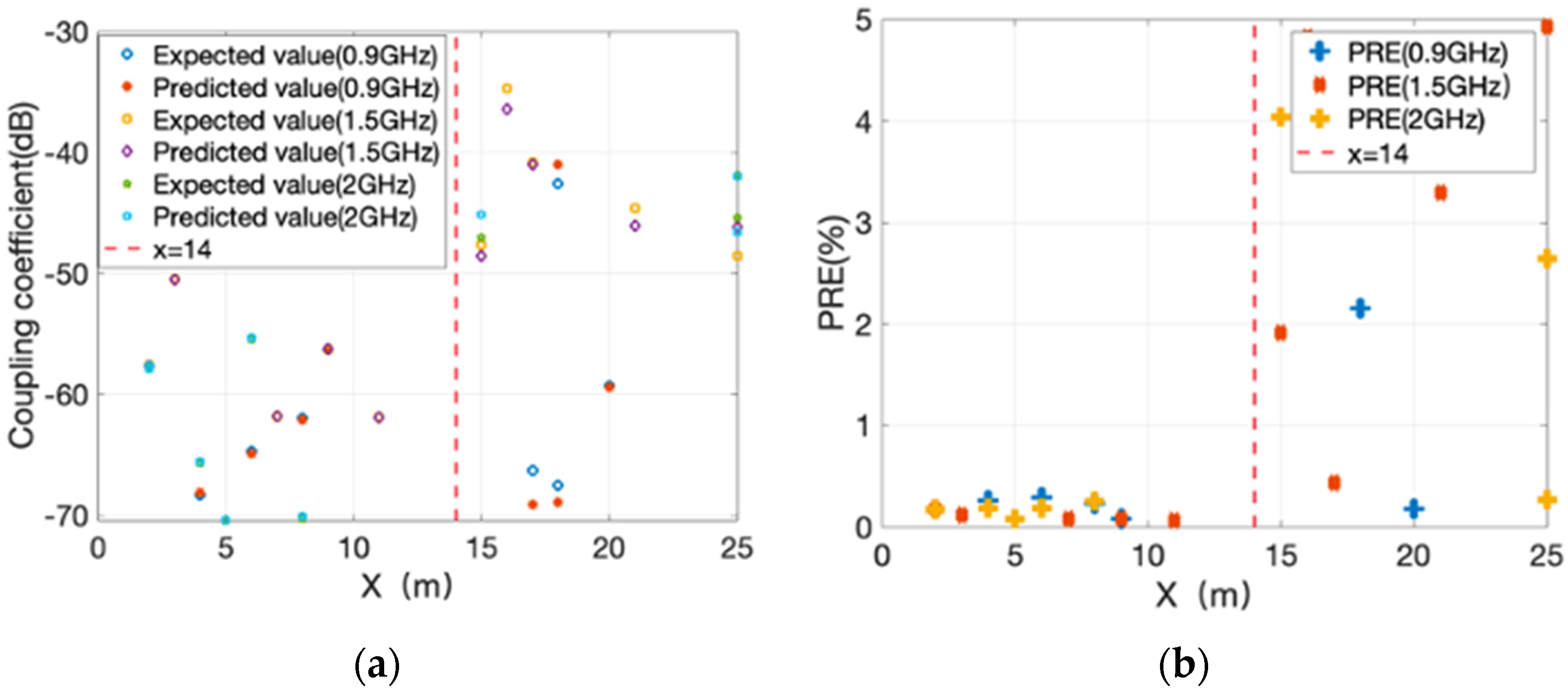
In addition, among the 10 predictions, sub-neural network 3 has a higher prediction accuracy for two times, which is because the optimization algorithm sometimes gives poor initial parameters compared with the initial parameters generated randomly, which is not uncommon in the application of optimization algorithms [21]. When 3 m < X ≤ 14 m, the RPEMax of sub-neural network 1 and sub-neural network 2 are 1.90% and 0.33%, respectively, and the other two prediction performance indices of sub-neural network 2 are also smaller; that is, the prediction accuracy is better, which reflects the role of the optimization algorithm MEA. Therefore, in MNN1, X = 3 m is taken as the dividing line, and the integration strategy is set as, when X ≤ 3 m, the prediction model based on sub-neural network 1 is used for prediction, and, when X > 3 m, the prediction model based on sub-neural network 2 is used for prediction, and the two outputs are optimized to obtain the prediction result of MNN1. The prediction results of the MNN1 prediction model are shown in Figure 8.
The comparison of the MNN1 prediction results based on the X direction of the horizontal co-ordinate is shown in Figure 8a, and the corresponding PRE is shown in Figure 8b. In order to present the prediction results clearly, only 25 coupling coefficients are randomly selected in the figure. From Figure 8, it can be seen that, when X ≤ 14 m, the predicted value and expected value of the MNN1 prediction model are relatively close, indicating that the prediction accuracy of MNN1 is high. This can be verified by the results in Figure 8a. However, it can also be seen from the prediction error distribution in the X direction in Figure 8a that, when X > 14 m, the prediction error of the MNN1 prediction model is large, and PREMax is about 3.33%. The overall prediction results are shown in Table 6.
In summary, the MNN1 prediction model based on the piecewise prediction strategy can achieve a higher prediction accuracy when X ≤ 14 m, but, when X > 14 m, its prediction accuracy is poor, so it is necessary to introduce a more suitable prediction model to supplement it, so as to obtain more accurate results.

3.6.2. Prediction Results and Errors of MNN2 Prediction Model

As mentioned above, in this paper, when Y = 0.8 m is taken as the dividing line in MNN2, the sub-neural network 3 prediction model and sub-neural network 4 prediction model are constructed based on the ELM algorithm and PSO-ELM algorithm, respectively, when Y > 0.8 m and Y ≤ 0.8 m. Similarly, the optimal number of neurons in the hidden layer of the ELM algorithm was determined by the trial-and-error method, and the parameters of the PSO-ELM algorithm are shown in Table 7. The prediction results are shown in Table 8.
As can be seen from Table 8, when Y > 0.8 m, the PERMax of sub-neural network 3 (Sub-NN3) and sub-neural network 4 (Sub-NN4) in MNN2 are 2.11% and 1.93%, respectively, and the other two prediction performance indices are similar. However, the prediction model of sub-neural network 3 is only based on the ELM algorithm and does not need to be combined with PSO, and the structure of the prediction model is simpler, so it has better engineering practicability.
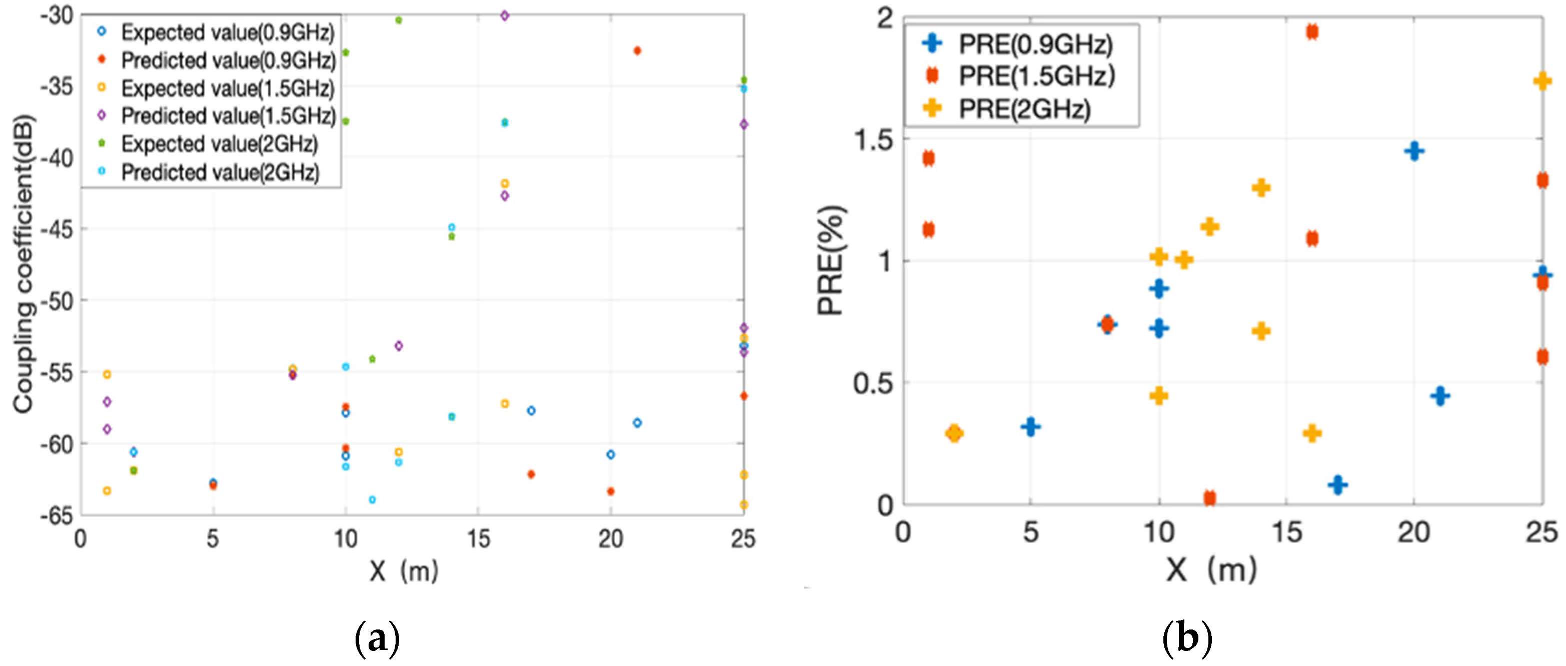
As above, among the 10 predictions, sub-neural network 3 has a higher prediction accuracy for one time, which also shows the instability of the prediction model constructed by the PSO-ELM algorithm. When Y < 0.8 m, the PREMax of sub-neural network 3 and sub-neural network 4 are 3.32% and 2.14%, respectively, and the other two prediction performance indices of sub-neural network 4 are also smaller, achieving a higher prediction accuracy, which reflects the role of the optimization algorithm PSO. Therefore, in this paper, Y = 0.8 m is taken as the dividing line in MNN2, and the integrated strategy is used to establish a prediction model based on sub-neural network 3 when Y ≥ 0.8 m. When Y < 0.8 m, a prediction model is established based on sub-neural network 4, and the output of the two is optimized, and the prediction result of MNN2 is finally obtained. The corresponding RPE is shown in Figure 9.
As can be seen from Figure 9a, the predicted value and expected value of the prediction model based on MNN2 are close to each other, and, as can be seen from Figure 9b, the prediction accuracy of MNN2 is relatively average. From the comparison between Figure 8 and Figure 9, it can also be seen that, when X ≤ 14 m, the RPEMax of MNN1 and MNN2 are approximately 0.31% and 1.95%, respectively. But, when X > 14 m, RPEMax is approximately 3.33% and 2.12%, respectively, the prediction accuracy of MNN2 is higher, and the overall prediction results are shown in Table 9.
In summary, MNN1 and MNN2 can complement each other to construct a more accurate prediction model.

3.6.3. Prediction Results and Errors of Prediction Model Based on MMNN

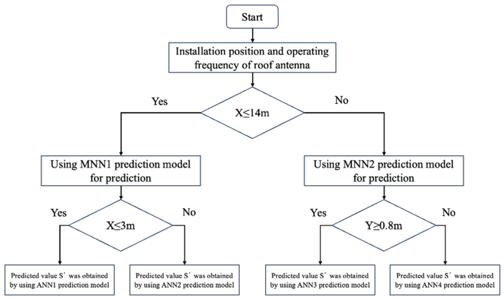
In this paper, the “selective” multi-mode fast strategy is adopted to construct the prediction model. In combination with the above comparison and analysis of the prediction results of the two sub-module prediction models, when X ≤ 14 m, the prediction accuracy of the MNN1 prediction model is higher, and, when X > 14 m, the prediction accuracy of the MMN2 prediction model is higher. Therefore, in order to further improve the prediction accuracy of the prediction model, this paper adopts the block prediction method; that is, the block integration strategy is used to optimize the output of the prediction results of MNN1 and MNN2, so as to build the prediction model of the coupling coefficient based on the MMNN. The main structure of the prediction model is shown in Figure 10. There are three steps in the model construction process.
For the first step, when the installation position and working frequency of a set of roof antennae are input into the prediction model, the prediction model will first determine whether the horizontal co-ordinate X ≤ 14 m is in the installation position. If the judgment result is “Yes”, the prediction model will choose the MNN1 prediction model for prediction.
In the second step, when MNN1 is selected, it will further determine whether X ≤ 3 m, and then select the prediction result of sub-neural network 1 or sub-neural network 2 as the final prediction result of MNN1.
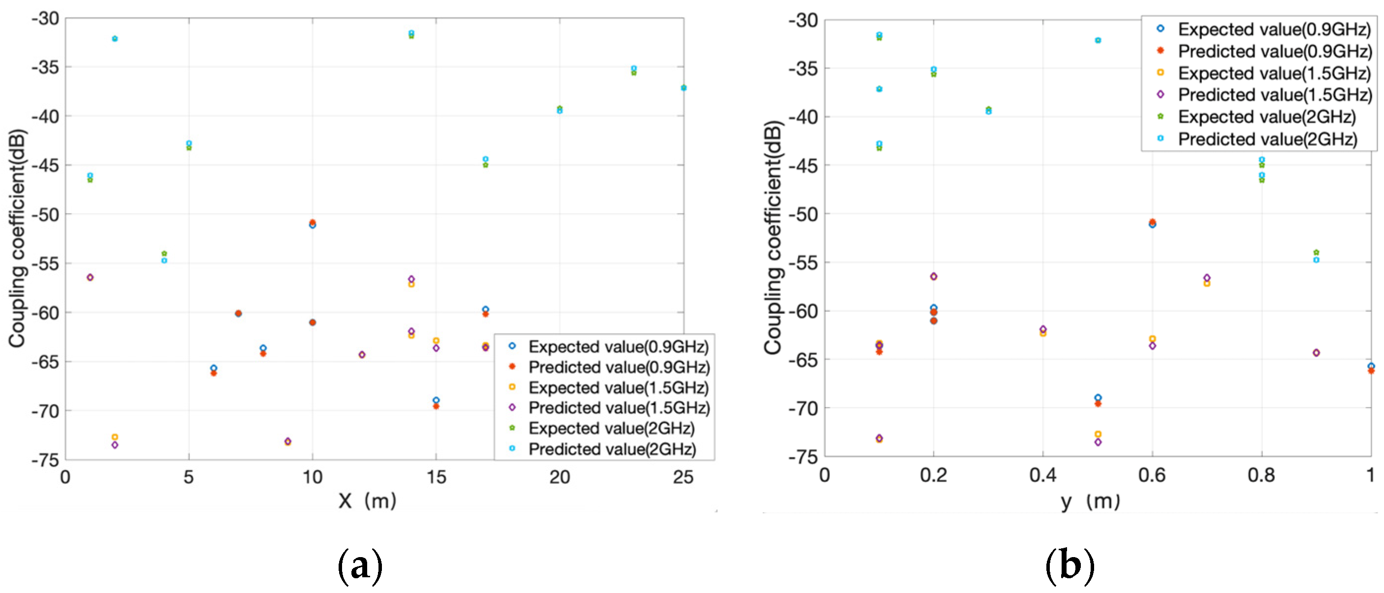
In the third step, if X > 14 m, the prediction model will select MNN2 for the prediction analysis. As mentioned above, Y = 0.8 m will be further used as the dividing line for MNN2 to judge, and the prediction result of sub-neural network 3 or sub-neural network 4 will be selected as the final prediction result of MNN2. Through a further comparative analysis of the prediction results of the proposed MMNN prediction model and the prediction results of four single neural networks, it can be seen that the prediction accuracy of the prediction model based on the MMNN has been significantly improved, and the prediction results will be analyzed in detail below. The prediction results and PRE of the prediction model based on the MMNN are shown in Figure 11 and Figure 12, respectively, and their three prediction performance indices are shown in Table 10. The four single neural networks mentioned above are also used as comparison models in this paper, and their three prediction performance indices are shown in Table 11.
From the comparison of the results in Figure 11 and Figure 12, it can be seen that, at each different co-ordinate, the predicted value and expected value of the prediction model based on the MMNN are very similar, and the PRE is very low; that is, the prediction accuracy is very high. As can be seen from Table 10, for roof antennae with three different operating frequencies, the prediction model based on the MMNN has similar performance indices, with the maximum values being MSEMax = 0.003, MAEMax = 0.040, and PREMax = 2.01. This fully proves that the prediction model established in this paper has a high accuracy when facing different roof antennae. As can be seen from Table 11, the MSE = 0.002, MAE = 0.033, and PREMax = 1.52% of the prediction model based on the MMNN are the lowest compared with the other four prediction models, which fully proves the accuracy of the prediction model established in this paper. The prediction performance indices of the MEA-BP prediction model compared to the BP prediction model and the PSO-ELM prediction model compared to the ELM prediction model have all decreased, proving the effectiveness of the optimization algorithm.
Next, the required computing time and occupied computer storage space obtained after a single prediction and a single electromagnetic simulation are given, as shown in Table 12.
As can be seen from Table 12, the PRE of the prediction model based on the MMNN proposed in this paper is only 2.01%, and, compared with the electromagnetic simulation method, the operation time only accounts for about 1/40 of the electromagnetic simulation time, and the storage space is also greatly saved. That is, when the prediction model ensures the prediction accuracy, it also saves a lot of computing time and storage space, and can effectively replace the complicated electromagnetic simulation work, so as to realize the rapid optimization analysis of the installation position of the 5G-R antenna.

4. Conclusions

In order to improve the anti-interference performance of the 5G-R roof antenna, the electromagnetic coupling of the pantograph arcing to the roof antenna port is reduced. Taking the 5G-R roof antenna as an example, this paper quickly optimized the installation position of the antenna, and proposed a coupling coefficient prediction model based on the MMNN. The MMNN model based on BP, MEA-BP, ELM, and PSO-ELM is used to predict the coupling coefficient between the pantograph arcing and the port of the roof antenna. It is proven that the prediction model can replace the complicated electromagnetic simulation work accurately and efficiently through various prediction performance indices, so as to provide an effective prediction method for the rapid optimization of the installation position of the roof antenna.
However, the simulation model is a simplified model. The structure of the body of the carriage is equivalent to a rectangular structure in the model. In order to further improve the prediction accuracy, the relevant parameters in the simulation model should be modified by the measured data. Through the continuous cycle iteration of simulation analysis and actual measurement verification, the further optimization of the installation position of the 5G-R antenna is realized.

Author Contributions

Conceptualization, Y.W. and Y.B.; methodology, Y.B. and J.R.; software, Y.B.; validation, Y.B. and J.R.; formal analysis, Y.B.; investigation, Y.B.; resources, Y.B.; data curation, Y.B.; writing—original draft preparation, Y.B.; writing—review and editing, J.R. and Y.B.; funding acquisition, Y.W. All authors have read and agreed to the published version of the manuscript.

Funding

This research was funded by the National Key Research and Development Program of China (2022YFB4301203-09).

Institutional Review Board Statement

Not applicable.

Informed Consent Statement

Not applicable.

Data Availability Statement

The raw data supporting the conclusions of this article will be made available by the authors on request.

Conflicts of Interest

The authors declare no conflicts of interest.

References

  1. He, X.; Wen, Y.; Zhang, D. A Fast Prediction Method for the Electromagnetic Response of the LTE-R System Based on a PSO-BP Cascade Neural Network Model. Appl. Sci. 2023, 13, 6640. [Google Scholar] [CrossRef]
  2. Ma, L. The Radiated Characteristics of Pantograph Arcing in High-speed Railway. Ph.D. Thesis, Beijing Jiaotong University, Beijing, China, 2018. [Google Scholar]
  3. Mariscotti, A.; Marrese, A.; Pasquino, N. Time and frequency characterization of radiated disturbances in telecommunication bands due to pantograph arcing. In Proceedings of the Instrumentation & Measurement Technology Conference, Graz, Austria, 13–16 May 2012; pp. 2178–2182. [Google Scholar]
  4. Ma, L.; Wen, Y.; Marvin, A.; Karadimou, E.; Armstrong, R.; Cao, H. A Novel Method for Calculating the Radiated Disturbance from Pantograph Arcing in High-speed Railway. IEEE Trans. Veh. Technol. 2017, 66, 8734–8745. [Google Scholar] [CrossRef]
  5. Tang, Y. Research On Model Characteristics and EMI of Pantograph-Catenary Arc of the High Speed Train. Ph.D. Thesis, Southwest Jiaotong University, Chengdu, China, 2021. [Google Scholar]
  6. Wang, S. Research on Time Domain and Time Domain Propagation Characteristics of Electric Field Noise Radiated from Pantograph-Catenary Arc. Master’s Thesis, Liaoning Technical University, Fuxin, China, 2019. [Google Scholar]
  7. Shan, Q. Research on Key Techniques of Electromagnetic Compatibility for the China Railway High-Speed. Ph.D. Thesis, Beijing Jiaotong University, Beijing, China, 2013. [Google Scholar]
  8. Wang, J. The Influence of Pantograph Arcing Radiation Disturbance on Communication Quality of LTE-R. Master’s Thesis, Beijing Jiaotong University, Beijing, China, 2020. [Google Scholar]
  9. Zhang, S. Method for Predicting Electromagnetic Response of Sensitive Equipment Based on Neural Network. Master’s Thesis, Beijing Jiaotong University, Beijing, China, 2021. [Google Scholar]
  10. Ling, S. Research on Coverage Technologies of New Generation Wideband Railway Mobile Communications and Their Applications in Trial Systems. Ph.D. Thesis, Nanjing University of Posts and Telecommunications, Nanjing, China, 2022. [Google Scholar]
  11. Xu, H. Research on Key Technologies and Resource Allocation Algorithms of High Speed Railway Wireless Communication based on 5G. Ph.D. Thesis, China Academy of Railway Sciences, Beijing, China, 2022. [Google Scholar]
  12. Song, Y.; Wen, Y.; Zhang, D.; Lin, S.; Wang, W. Fast Prediction Model of Coupling Coefficient Between Pantograph Arcing and GSM-R Antenna. IEEE Trans. Veh. Technol. 2020, 69, 1612–11618. [Google Scholar] [CrossRef]
  13. Pu, S. Integrative Modelling and Analysis of Radio Frequency Link for Wireless Communication in Railway Environments. Ph.D. Thesis, Beijing University of Technology, Beijing, China, 2011. [Google Scholar]
  14. Li, D. Research on the Radio Coverage Characteristics in Confined Space. Ph.D. Thesis, Beijing University of Technology, Beijing, China, 2016. [Google Scholar]
  15. Dou, Y.; Li, Y.; Li, H.; Bao, J.; Lin, W. Isolation between Vehicle-Mounted Antennas for 350 km/h Chinese Standard EMU and Minimum Spacing. Chin. Railw. Sci. 2021, 42, 130–136. [Google Scholar]
  16. Dong, G.; Li, Y.; Li, H.; Bao, J.; Lin, W. Research on Performance and Interference Isolation of EMU’s Roof-mounted 450 MHz Frequency Band Antennas. Railw. Sign. Comm. 2021, 57, 42–47. [Google Scholar]
  17. Zhu, Q.; Chen, S. Shipboard Antennas Layout Based on Multi-Objective Optimization Algorithm. Sh. Sci. Technol. 2014, 36, 132–135. [Google Scholar]
  18. Song, Y.; Wen, Y.; Zhang, J.; Zhang, D. Fast Prediction Model for the Susceptibility of Balise Transmission Module System Based on Neural Network. In Proceedings of the 2019 International Conference on Electromagnetics in Advanced Applications, Granada, Spain, 9–13 September 2019; pp. 0445–0448. [Google Scholar]
  19. Wei, M. Research on Current Distribution and Control Strategy of Hybrid Excitation Synchronous Motor Speed Control System. Master’s Thesis, Xi‘an University of Technology, Xi’an, China, 2023. [Google Scholar]
  20. Zhang, W. Research on Fast Simulation Method of electromagnetic radiation of Arc between Pantograph and Catenary. Master’s Thesis, Liaoning Technical University, Fuxin, China, 2023. [Google Scholar]
  21. Wang, X. Analysis of 43 Cases of MATLAB Neural Networks, 1st ed.; Beihang University Press: Beijing, China, 2013; pp. 11–18. [Google Scholar]
  22. Sun, C.; Sun, Y.; Xie, K. Mind-evolution-based machine learning and applications. In Proceedings of the 3rd World Congress on Intelligent Control and Automation, Hefei, China; 2000; pp. 112–117. [Google Scholar]
  23. Wang, X.; Lin, Q.; Wu, H.; Zhao, P. Large Signal Modeling Method Based on MEA-BP Neural Network. In Proceedings of the International Conference on Microwave and Millimeter Wave Technology (ICMMT), Harbin, China, 12–15 August 2022; pp. 1–3. [Google Scholar]
  24. Zhu, Z.; Pang, Y.; Chen, Y. A Fault Diagnosis Method for Satellite Reaction Wheel Based on PSO-ELM. In Proceedings of the 2022 41st Chinese Control Conference (CCC), Hefei, China, 25–27 July 2022; pp. 4002–4007. [Google Scholar]
  25. Lu, C. Research on Design of Self-Organizing Modular Neural Network and Its Applications on Wastewater Detection. Ph.D. Thesis, Beijing University of Technology, Beijing, China, 2018. [Google Scholar]
  26. Song, Y. Research and Application on Electromagnetic Coupling of Vehicle Antenna of High-Speed Train Based on Artificial Intelligence. Ph.D. Thesis, Beijing Jiaotong University, Beijing, China, 2022. [Google Scholar]
  27. Zhang, Z. The Study Of Self-Organization Modular Neural Network Architecture Design. Ph.D. Thesis, Beijing University of Technology, Beijing, China, 2013. [Google Scholar]
Figure 1. A simplified model for the coupling coefficient of pantograph arcing and GSM-R antenna.
Applsci 14 06954 g001
Figure 3. Antenna pattern of the roof antenna with two installation positions (f = 2 GHz) (red line is the pattern of the radiation field strength of the antenna changing with direction, and the interval between the two blue lines is the main lobe width): (a) coupling coefficient (Max); and (b) coupling coefficient (Min).
Applsci 14 06954 g003
Figure 4. Modular modeling diagram.
Applsci 14 06954 g004
Figure 5. The specific flow block diagram of the MEA-BPNN.
Applsci 14 06954 g005
Figure 6. The specific flow block diagram of the PSO-ELM.
Applsci 14 06954 g006
Figure 7. Structure of the proposed MMNN prediction model.
Applsci 14 06954 g007
Figure 8. Prediction results and relative prediction error of MNN1 in X direction: (a) comparison results in X direction (coupling coefficient ranges from −70 to −30); and (b) PRE in X direction.
Applsci 14 06954 g008
Figure 9. Prediction results and relative prediction error of MNN2 in X direction: (a) comparison results in X direction (coupling coefficient ranges from −65 to −30); and (b) PRE in X direction.
Applsci 14 06954 g009
Figure 10. Structure of the proposed prediction model based on MMNN.
Applsci 14 06954 g010
Figure 11. Prediction results of the proposed prediction model based on MMNN: (a) comparison results in X direction (coupling coefficient ranges from −75 to −30); and (b) comparison results in Y direction (coupling coefficient ranges from −75 to −30).
Applsci 14 06954 g011
Figure 12. PRE of the proposed prediction model based on MMNN: (a) comparison results in X direction; and (b) comparison results in Y direction.
Applsci 14 06954 g012
Table 1. Comparison of the two coupling coefficients.
Installation Position
(X, Y) (m)
Port of Monopole Antenna (1.268 GHz) Port of Monopole Antenna (2 GHz)
(3, 0)−43.52 dB−50.21 dB
(5, 0)−41.82 dB−58.55 dB
(3, 0.5)−49.27 dB−63.46 dB
Table 2. Partial data of coupling coefficient.
Position (X, Y) (m)Frequency (GHz)Coupling Coefficient (dB)
1, 00.9−59.9
25, 00.9−65.4
24, 12.0−63.8
25, 12.0−53.7
Table 4. Comparison of the performances of roof antennae at different installation positions.
Frequency
(GHz)
Coupling Coefficient (Max)Coupling Coefficient (Min)
Position
(X, Y) (m)
MLA (dBi)MLD (°)Position
(X, Y) (m)
MLA (dBi)MLD (°)
0.920, 0.44.9671.014, 0.85.2462.0
1.525, 0.14.9861.015, 0.85.0065.0
2.03, 0.46.8165.015, 0.26.7350.0
Table 5. Comparison of coupling coefficients of roof antennae with different operating frequencies.
X ≤ 3 m 3 m < X ≤ 14 m
MSE MAE PREMax MSE MAE PREMax
Sub-NN1
(BP)
0.0050.0630.28%0.2120.3851.90%
Sub-NN2
(MEA-BP)
0.0050.0550.31%0.0060.0660.33%
Table 6. Performance comparison 2 of prediction models (MNN1).
X ≤ 14 m14 m < X ≤ 25 m
MSEMAEPREMaxMSEMAEPREMax
MNN10.0090.0810.31%1.0620.8633.33%
Table 7. Parameters of the PSO-ELM algorithm.
ParametersValue
Acceleration factor c12.49445
Acceleration factor c22.49445
Number of iterations200
Maximum velocity1
Minimum velocity−1
Maximum position5
Minimum position−5
Table 8. Performance comparison 1 of prediction models (MNN2).
0.8 m ≤ Y ≤ 1 m (14 m < X ≤ 25 m)Y < 0.8 m (14 m < X ≤ 25 m)
MSEMAEPREMaxMSEMAEPREMax
Sub-NN3
(ELM)
0.0030.0412.11%0.0060.0723.32%
Sub-NN4 (PSO-ELM)0.0010.0321.93%0.0030.0432.14%
Table 9. Performance comparison 2 of prediction models (MNN2).
X ≤ 14 m14 m < X ≤ 25 m
MSEMAEPREMaxMSEMAEPREMax
MNN20.3610.5111.95%0.4380.5572.12%
Table 10. Performance comparison of prediction model for three kinds of roof antennae.
Frequency (GHz)MSEMAEPREMax
0.90.0030.0371.90%
1.50.0030.0402.01%
2.00.0020.0331.52%
Table 11. Performance comparison of prediction models.
Prediction ModelMSEMAEPREMax
MMNN0.0020.0331.52%
BP0.0080.0733.23%
MEA-BP0.0040.0562.51%
ELM0.0050.0603.06%
PSO-ELM0.0040.0582.35%
Table 12. Performance comparison of electromagnetic simulation and prediction model.
Computation TimeStorage SpaceCoupling Coefficient (dB)PRE
Electromagnetic simulation41 min352 MB−60.212.01%
Prediction model (MMNN)68 s3.2 MB−61.42
Disclaimer/Publisher’s Note: The statements, opinions and data contained in all publications are solely those of the individual author(s) and contributor(s) and not of MDPI and/or the editor(s). MDPI and/or the editor(s) disclaim responsibility for any injury to people or property resulting from any ideas, methods, instructions or products referred to in the content.