Supervised Machine Learning Models for Mechanical Properties Prediction in Additively Manufactured Composites

Abstract

This paper analyses mechanical property prediction through Machine Learning for continuous fiber-reinforced polymer matrix composites printed using the novel Material Extrusion Additive Manufacturing technique. The composite is formed by a nylon-based matrix and continuous fiber (carbon, Kevlar, or fiberglass). From the literature, the elastic modulus and tensile strength were taken along with printing parameters like fiber content, fiber fill type, matrix lattice, matrix fill density, matrix deposition angle, and fiber deposition angle. Such data were fed to several supervised learning algorithms: Ridge Regression, Bayesian Ridge Regression, Lasso Regression, K-Nearest Neighbor Regression, CatBoost Regression, Decision Tree Regression, Random Forest Regression, and Support Vector Regression. The Machine Learning analysis confirmed that fiber content is the most influential parameter in elasticity (E) and strength ($\sigma$). The results show that the K-Nearest Neighbors and CatBoost provided the closest predictions for E and $\sigma$ compared to the other models, and the tree-based model presented the narrowest error distribution. The computational metrics point to a size versus prediction time tradeoff between these two best predictors, and adopting the prediction time as the most relevant criterion leads to the conclusion that the CatBoost model can be considered, when compared to the others tested, the most appropriate solution to work as a predictor in the task at hand.

1. Introduction

Additive Manufacturing (AM) is a rapidly growing area [1,2]. By 2024, the market is expected to reach USD 24 billion [3]. On the other hand, composite materials offer the high directional strength of fiber reinforcement with the flexibility of an adaptable matrix [2,4]. Technologies, such as the Markforged Two^® printer [5], blend the best features of composites and AM [6], giving those materials load-bearing capabilities that can match that of Aluminum [7]. AM could be the technology that closes the gap between topological optimization and actual fabrication [8] because of its unique ability to manufacture many lattices and intricate geometries [9]. However, designers must have appropriate mechanical properties to implement such a flexible technique in components.

Markforged^® [5] filed a patent in 2015 for a device that used Material Extrusion (MEX) to manufacture continuous fiber composites. A schematic of the composite MEX printing process is shown in Figure 1. MEX, arguably the most popular of the AM technologies [10], is a manufacturing technique in which the topology is reconstructed layer by layer from a G-code file previously converted to the Standard Template Library language. For Markforged^® composites, this process is performed by a software in the cloud called Eiger^® [5].

The options to create a part using the Markforged^® technology are broad in number and range. Their impact has been documented [2,4,11,12,13]. The options are the type of continuous fiber (carbon, Kevlar, fiberglass, and high-temperature fiberglass), fiber volume fraction ($V_f$), fiber fill type (concentric and isotropic, as seen on the top of Figure 2), the pattern of matrix filling (hexagonal, triangular, square, as seen at the bottom of Figure 2, and solid fill), matrix fill density, matrix deposition angle, and fiber deposition angle. The mechanical characterization for different matrix fillings from geometry and material properties is thoroughly reviewed in [4,11]. Markforged, the sole provider of matrix and fiber, has characterized individual mechanical properties for matrix (Nylon and Onyx^®) and continuous fibers, as seen in

Table 1. Mechanical properties as provided by Markforged [5]. E is elastic modulus, $\sigma$ is strength, and $ϵ$ is strain.

Material	E [GPa]	$\mathit{\sigma }$ [MPa]	$\mathit{ϵ}$ %
Nylon	1.7	33.5	4.5
Onyx	1.4	36	33
Standard	ASTM D638 [16]	ASTM D638 [16]	ASTM D638 [16]
Carbon	60	800	1.5
Fiberglass	21	590	3.8
Kevlar	27	610	2.7
Standard	ASTM D3039 [17]	ASTM D3039 [17]	ASTM D3039 [17]

. It has to be noted that Onyx^® is a composite itself, a nylon matrix reinforced with chopped carbon fiber. Thus, it shows multiple options and ranges to configure a part.

Predicting the material properties is still a challenge. The available prediction models for mechanical properties do not include all the variables [18,19], a task that has to be performed experimentally [11,13,20,21] or numerically [15,18]. However, the existing numerical modeling requires highly skilled users, a deep understanding of the mechanical behavior of composite materials, and fairly advanced numerical modeling skills [18,19,22,23,24]. Such requirements are mainly due to the composite’s nature on top of the intrinsic anisotropy of AM. In order to ease the task, the authors of [4] suggested modeling mechanical performance for this kind of composite as isotropic materials with bulk mechanical properties obtained from mechanical testing and linking them to the printing variables. Therefore, the need for a model to predict mechanical properties (strength and elasticity), including the printing variables, or at least the most representative, arises. This way, a novice user can design a component using a simple isotropic numerical model. The Volume Average Stiffness (VAS) model [19] is based on the Rule of Mixtures (ROM), but it accounts for each region of the cross-sectional area. In addition, it accounts for the infill-type adopting models proposed by Gibson and Ashby [25] for cellular materials and the composite’s anisotropy. Recently, the authors of [15,26] applied the VAS method, including porosity and the Tsai–Hill equations, to predict mechanical properties. It was acknowledged that developing a numerical model with individual properties (fiber and matrix) takes advanced skills. The model requires a deep understanding of composite theory [27] to be adopted, which may impede the popularization of the printing technique. On the other hand, Machine Learning (ML) has been extensively used and applied in different areas and applications. Therefore, ML could link printing variables and mechanical properties.

When focusing on AM, there are plenty of works that make use of data-driven methods to predict material properties [28,29]. In conventional manufacturing, Artificial Intelligence (AI) has been applied to predict surface roughness, welds, forging, geometric tolerance, sheet metal, and quality control in AM parts [30].

On the other hand, AI systems have the ability to recognize patterns, identify trends within data, and categorize them based on such patterns. Although AI may be exceptionally good at pattern recognition, it has limits, such as sensitivity to biases in training data and its limitation to generalize beyond known patterns. Furthermore, several works have focused on applying ML to predict material’s mechanical response [29]. Ng et al. [28] reviewed how authors explored the Artificial Neural Network (ANN) in ML. Tavares [31] used an ANN to predict static properties of dual-phase steel from processing and chemical composition. Furthermore, [32] cited several cases where ML was used for strength, stiffness, and strain prediction. Finally, in composites, ML techniques have been used for composites, including the manufacturing method, simulation, and mechanical testing as data input to search for a constitutive model as a whole or a Representative Unit Cell (RUC) [33,34].

Now, more specifically in AM, ML has been used extensively as well. Zhang et al. [35] used ANNs to predict the mechanical behavior of the Fused Deposition Modeling (FDM) of polymer parts accounting for temperature, printing speed, and layer height. León et al. [36] used several machine learning algorithms to predict elastic modulus and strength based on selected printing parameters. The study concluded that fiber angle and fiber content are the factors with the most influence on stiffness and strength. However, the $R^2$ for their prediction was as low as 0.19 for a fine tree network and 0.66 for the Matern 5/2 Gaussian Process Regression model, whereas a micromechanic-based model gave a $R^2$ of 0.74. One can see that there is still room for improvement. Modeling mechanical properties with the existing methods is rather complex due to the large number of variables involved (see Figure 2). To use homogenization such as for a representative volume unit and others, one needs advanced numerical skills. This could be a roadblock to popularizing the use of AM composites. Therefore, the present paper attempts to ease that task by predicting mechanical properties using ML methods.

1.1. Contributions

Based on the recently published research in the intersection of AM, ML, and mechanical property prediction, one can highlight the following main contributions of this work:

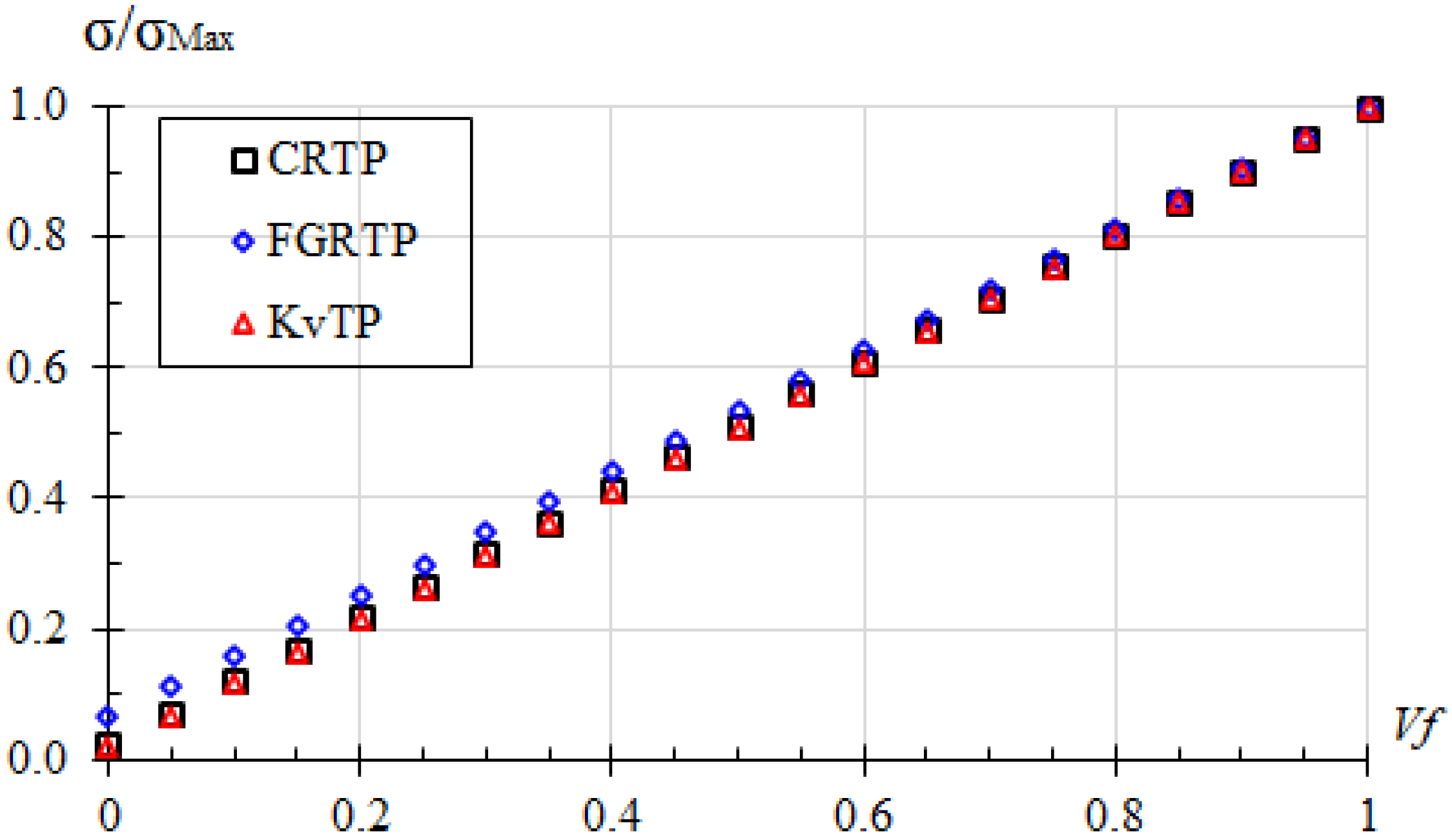
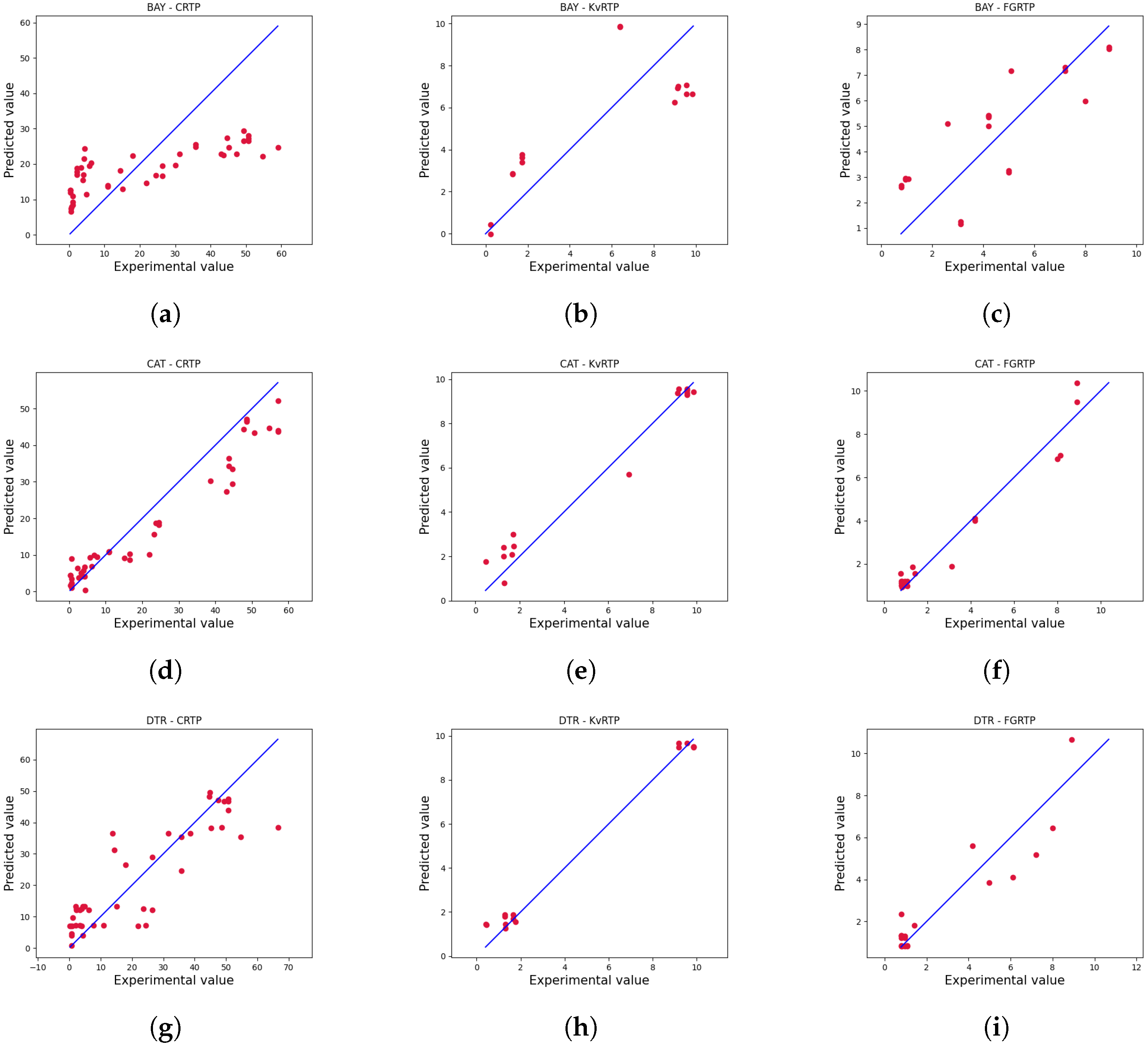
• A ML pipeline that estimates mechanical properties such as the strength and elasticity of AM composite materials reinforced with continuous fibers—carbon (CRTP), Kevlar (KvRTP), and fiberglass (FGRTP).
• A dataset was constructed from the peer-reviewed literature. It includes mechanical properties (elasticity and strength), materials for continuous fibers, and printing parameters. A robust analysis and the greater reliability of the ML models that have been tested enable the reproducibility and exploration of polymer-based AM technologies.
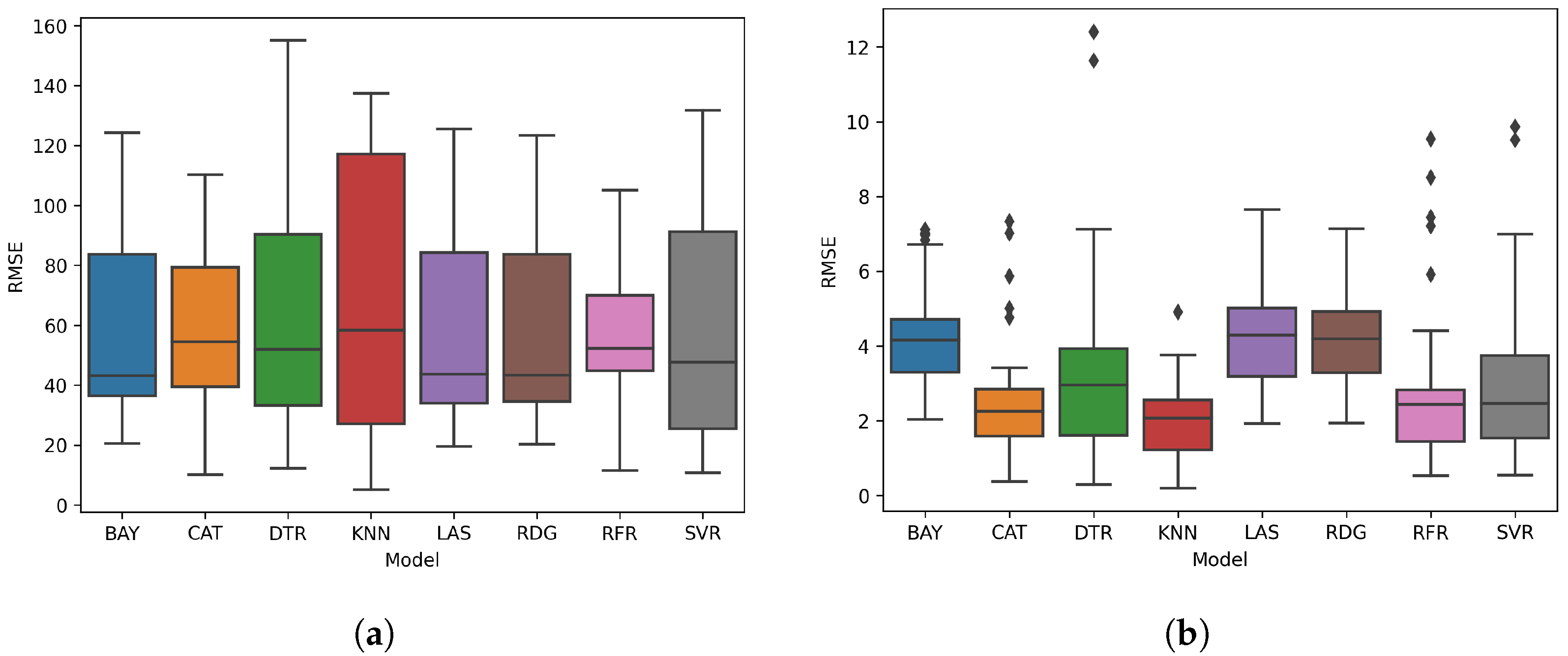
• In order to determine the most efficient ML models for predicting mechanical properties, this paper examines a variety of linear and nonlinear ML models. The performance analysis reveals their strengths and weaknesses when used within the AM context. As new algorithms are developed, they can be tested with the existing dataset. The modeling workflow used comprises k-fold cross-validation and Monte Carlo resampling, exploring different lightweight machine learning methods like Bayesian Ridge Regression (BAY), CatBoost Regression (CAT), Decision Tree Regression (DTR), k-nearest Neighbors (KNN), Lasso Regression (LAS), Random Forest Regression (RFR), Ridge Regression (RDG), and Support Vector Regression (SVR).
• The manuscript shows how decisive printing parameters are, such as deposition angles and fiber content, for the mechanical properties of Continuous Fiber Reinforced Polymer Matrix Compositess (CFRPCs). Therefore, the results can be used to optimize material properties without conducting extensive experimental campaigns. The identification of such parameters should lead to a more efficient design anddevelopment process.

Moreover, when applying ML to AM mechanical property prediction, there are implications such as enhanced design capabilities (i), personalized material selection (ii), reduction in experimental campaign development time (iii), and scalability and production efficiency (iv). (i) A designer can maximize a CFRPC component by reducing the uncertainty in the mechanical property prediction. This could result in the manufacture of lightweight, high-strength components designed for tailored purposes, improving the overall performance of AM products. (ii) This study emphasizes the importance of various parameters, such as deposition angles and fiber content, that influence the mechanical properties of AM composites. With this in mind, a designer can select materials, in combination with AM parameters, to customize a tailored component more effectively, thus ensuring that the final part meets the requirements and performance standards. (iii) Experimental testing can be costly and time-consuming. By using ML models, manufacturers can lower the costs associated with material testing, thus speeding up the development process. (iv) The results indicate that ML can help popularize AM processes by demystifying the knowledge on how to best optimize printing parameters to achieve a mechanical property target.

1.2. Paper Organization

The remainder of this paper is organized as follows. Section 2 addresses the essential technical background encompassing the scope of this work. Section 3 describes the methods and dataset adopted. Finally, Section 4 shows and analyzes the results, while Section 5 summarizes this study’s main findings.

2. Technical Background

2.1. Models to Predict AM Composites’ Elasticity

To predict mechanical properties in composite materials, one can use the ROM from individual properties of the matrix and fiber [27]. For example, the elastic modulus E of a component is described in (1) for the direction parallel to the fiber, and in (2), for the direction perpendicular to the fiber:

$$E_{c_1}=E_f{V}_f+(1-V_f)E_m$$

(1)

$$E_{c_2}={\left[{\displaystyle \frac{V_f}{E_f}}+{\displaystyle \frac{1-V_f}{E_m}}\right]}^{-1}$$

(2)

where the subscript c refers to composite, f to fiber, m to the matrix, 1 to the parallel-to-the-fiber direction, and 2 to the perpendicular-to-the-fiber direction. Furthermore, if the porosity is to be accounted for, the elastic modulus is modified by the porosity level $p_1$, which is estimated at 10% [37]. Therefore, (3) shows the corrected elastic modulus.

$$E_1=\left(1-p_1\right)E_{c1}$$

(3)

On top of that, and because of the easiness of free-form fabricated AM components, cellular structures are commonly used. Figure 3 shows the RUC for the three cellular structures studied here. All lattices have a thickness t.

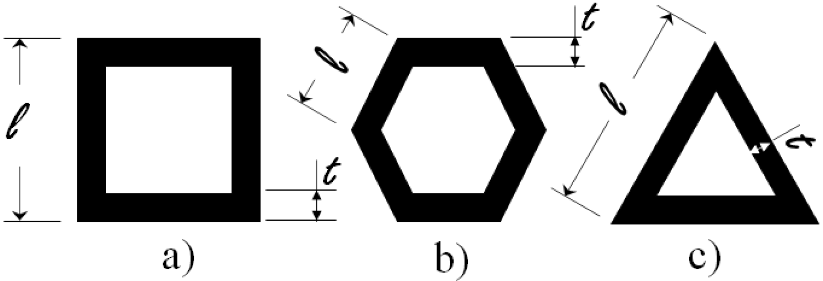
2.1.1. Square Lattice

The square lattice represents a good balance between the orthogonal strength and printing time. The RUC, in Figure 3a, is characterized by a square with side l. The infill density, ${\rho }_{sq}$, can be expressed as the ratio of the filled area to the total area, and it is given by (4), whereas the elastic modulus is given in (5) [25]. Note that density is the parameter that defines the geometry in Eiger^® software, https://www.eiger.io/.

$${\rho }_{sq}={\displaystyle \frac{-4t^{2}l+2tl}{l^2}}$$

(4)

$$E_1=E_s{\displaystyle \frac{t}{l}},$$

(5)

where $E_s$ represents the elastic modulus of the solid, and $E_1$ is the elastic modulus in the preferred fiber direction. When the axial load is aligned with the fiber, the x and 1 directions coincide.

2.1.2. Honeycomb or Hexagonal Lattice

The honeycomb lattice was developed mainly for compression applications, yielding a great strength-to-density ratio. The honeycomb pattern is characterized by a regular hexagon with side l, as shown in Figure 3b, and it is widely used as a core in manufacturing composite panels. It has good strength with fast printing times. The mechanical characterization of honeycomb structures can be found in [25], with elasticity presented in (6) and density in (7):

$$E_1=2.3E_s{\left({\displaystyle \frac{t}{l}}\right)}^3$$

(6)

$${\rho }_{Hex}={\displaystyle \frac{2t}{l\sqrt{3}}}$$

(7)

2.1.3. Triangular Lattice

The triangular lattice, as shown in Figure 3c, is used when strength is needed along the direction of the wall. It is stronger than the rectangular pattern but requires a longer printing time. The elasticity and density for an equilateral triangle are presented in (8) and (9), respectively.

$$E_1=1.15E_s{\displaystyle \frac{t}{l}}$$

(8)

$${\rho }_{Tr}={\displaystyle \frac{2\sqrt{3}t}{l}}$$

(9)

2.1.4. Solid Region

Because the solid is formed out of melted thermoplastic circular wire, there is porosity, named $p_1$, between adjacent extruder passes. Rodriguez et al. [37] proposed the porosity model for such regions, shown in (10). Note that elasticity is assumed as a solid but porous material, with $p_1$ values reported between 15 and 20% [38].

$$E_1=\left(1-p_1\right)E_s$$

(10)

A comparison of Equations (5), (6) and (8) is shown in Figure 4, where the normalized elastic modulus is plotted versus the variation in the thickness and length for the square, triangular, and hexagonal cellular structures. The elastic modulus is higher for a thick structure (larger t). Conversely, for a thin structure (smaller t), the triangular and square infills perform very similarly, whereas, for thicker structures, the hexagonal (honeycomb) becomes stiffer after a 0.65 t/L value.

The ROM model is simple and easy to implement but leaves out important variables that impact the AM composite prediction performance.

2.2. Models to Predict AM Composite Strength

On the other hand, in assuming that the composite abides by Hooke’s law, strength in the axial direction could be described by the ROM [27], as shown in (11):

$${\sigma }_{c_1}={\sigma }_f\left[V_f+{\displaystyle \frac{E_m}{E_f}}(1-V_f)\right],$$

(11)

where $\sigma$ is the tensile strength. Now, if we disregard the contribution of the matrix to withstand the load, (11) can be conservatively simplified to (12).

$${\sigma }_{c_1}={\sigma }_f{V}_f$$

(12)

The performance of the normalized composite´s normal strength, (11), using values from Table 1 is seen in Figure 5. Firstly, one can see that the variation is linear. Secondly, the prediction is very close for the three available fibers, especially at the upper limit of the volumetric fiber fraction. However, FGRTP provides a slightly higher strength at lower values because of the high rate $E_m/E_f$. Furthermore, there is evidence that an elevated volumetric fiber content leaves insufficient room for fiber/matrix adhesion [4,26], indicating that the ideal $V_f$ is between 40 and 50%.

2.3. Machine Learning Models

This section describes the machine learning methods adopted in this work. Since this is a supervised learning problem with a continuous label, only classical regression methods were selected.

2.3.1. Linear Regression

Linear regression is one of the simplest algorithms applied to solve regression problems. It assumes that the input variables have a linear relationship with the target variable. A straight line represents such a relationship in a two-dimensional space, i.e., when there is only one input variable, or it can be thought of as a hyperplane when the problem consists of more than one input variable. The mathematical representation of the linear regression model is presented in (13) [39]:

$$\widehat{y}=w_0+w_1{x}_1+w_2{x}_2+\cdots +w_p{x}_p,$$

(13)

where $\widehat{y}$ is the predicted value, $w_i$ denotes the coefficients of the model, and $x_i$ denotes the variables or features. Therefore, the Linear Regression (LR) algorithm consists of finding the coefficients of the model through an optimization process that aims to minimize a loss function, $J(y_i,{\widehat{y}}_i)$, defined as the sum of squares of the difference between the target and predicted values. This optimization technique is known as Ordinary Least Squares and is represented by (14):

$$J(y_i,{\widehat{y}}_i)=\sum _{i=0}^n{(y_i-{\widehat{y}}_i)}^2$$

(14)

Despite being simple and efficient, such a model can become sensitive to inputs and unstable, especially for problems with a small number of samples or fewer samples than features. One way to overcome this problem is to adopt a modified loss function that includes additional costs when there are many input variables. The additional portion of the modified loss function is called a penalty, and different types of penalty can be used, each of them defining a new algorithm included in the class of penalized linear regression models. These algorithms include the LAS, RDG, and BAY. The LAS refers to the penalization based on the sum of the absolute coefficient values, the so-called $L_1$ penalty, seen in (15). On the other hand, the RDG considers the $L_2$ penalty, which is defined as the sum of the squared coefficient values as seen in (16).

$$L_{1_{p}enalty}=\sum _{j=0}^p\left|w_j\right|$$

(15)

$$L_{2_{penalty}}=\sum _{j=0}^p{\left(w_j\right)}^2$$

(16)

Therefore, the modified loss functions for the RDG and LAS are defined in (18) and (17), respectively:

$$J_{Lasso}=J+\lambda ·L_{1_{penalty}}$$

(17)

$$J_{Ridge}=J+\lambda ·L_{2_{penalty}},$$

(18)

where $\lambda$ is a hyperparameter that weights the penalty applied to the loss function. The $\lambda$ values range from 0 to ∞, where 0 cancels the penalty, and large values leads to simpler models with fewer parameters. Furthermore, the BAY is similar to the classical RDG, with the difference that the regularization parameter is now tuned based on the dataset under analysis. Hence, the Bayesian model has the advantage of adapting to the data at hand, but with the drawback of the inference being possibly time-consuming.

2.3.2. CAT Boost Regression

The CAT algorithm was recently developed by Yandex, and it is perhaps one of the newest regression algorithms available nowadays. As the name suggests, CAT is based on decision trees [40] and gradient boosting [41]. The major features of the algorithm are its capacity to handle categorical variables and ordered boosting. The first refers to the ability not needing to perform any feature transformation before the training stage, which is generally mandatory for other algorithms. To do so, during the training stage, the CAT algorithm uses efficient modified target-based statistics [42]. The second major feature refers to the sequential construction of a set of base predictors so that each subsequent decision tree has a decreased loss [42]. Moreover, unlike traditional gradient boosting algorithms, CAT Boost grows oblivious trees as base predictors, i.e., trees with all nodes at the same level testing the same predictor with the same condition. Therefore, such characteristics make the CAT computationally efficient and less prone to overfitting [41].

2.3.3. K-Nearest Neighbors Regression

The K-Nearest Neighbors Regression is an instance-based algorithm primarily applied to solve regression problems. The core idea of the algorithm is quite simple: the predicted target value for a new instance is calculated by searching for the most similar samples in the dataset—the so-called neighbors—and computing the mean or median target value associated with them. Therefore, the only mathematics required are the calculus of distance metrics to find the neighbors of the query instance. Several distance measures can be used, such as the Euclidean (19), Manhattan (20), and Minkowski distances (21):

• Euclidean

  $$d(x_i,x_j)=\sqrt{{\left({\displaystyle \frac{}{}}{a}_r\left(x_i\right)-a_r\left(x_j\right)\right)}^2}$$

  (19)
• Manhattan

  $$d(x_i,x_j)=|a_r\left(x_i\right)-a_r\left(x_j\right)|$$

  (20)
• Minkowski

  $$d(x_i,x_j)={\left(|{\displaystyle \frac{}{}}{a}_r\left(x_i\right)-a_r\left(x_j\right){|}^p\right)}^{{\displaystyle \frac{1}{p}}},$$

  (21)

where $a_r\left(x\right)$ denotes the value of the $r_{th}$ feature. The most popular of them is the Euclidean distance.

The value of k, the number of neighbors to be considered, is the only hyperparameter of the model. It can be defined using hyperparameter tuning techniques, and typical values range from 1 to 21. Since the model relies on calculations conducted with the entire training data, its computational complexity considerably increases for large datasets [43].

3. Materials and Methods

3.1. Dataset

The data used in this study consist of a combination of datasets retrieved from a total of 26 studies recently published in the literature on composite AM. Because it is a new technology, there are not many tests yet. As one can see from the dataset presented in

Table 2. Dataset table representing groups of samples retrieved from several published works. The table shows the variations in the values of each feature used in this work.

Reference	Fiber Type	Fill Pattern	Fill Angle (°)	Fiber Angle (°)	Fiber Distrib.	${\mathit{V}}_{\mathit{f}}$	Properties
Blok [44]	C	T	$\pm 45$	$0,45$	NA	X	$E_1$, ${\sigma }_1$, ${\sigma }_{1c}$, G, ${\tau }_{12}$
Dutra [18]	C	NA	$\pm 45$	$0,90,\pm 45$	NA	X	$E_1$, ${\sigma }_1$, $E_2$, ${\sigma }_2$, $E_{1c}$, ${\sigma }_{1c}$, G, ${\sigma }_{12}$
Klift [45]	C	NA	0	NA	C	X	$E_1$, ${\sigma }_1$
Melenka [19]	Kv	NA	$\pm 45$	0	NA	NA	$E_1$, ${\sigma }_1$
Dickson [46]	C, Kv, FG	NA	NA	NA	C	NA	$E_1$, ${\sigma }_1$, $E_{1f}$,${\sigma }_{1f}$
Justo [47]	C, FG	NA	$\pm 45$	0, 90	NA	NA	$E_1$, $\sigma$, $E_{1c}$, ${\sigma }_{1c}$, ${\sigma }_{2c}$
Al-Abadi [48]	C, Kv, FG	NA	$\pm 45$	0, 90	C	NA	$E_1$, ${\sigma }_1$
Goh [13]	C, FG	NA	NA	0, 90, $\pm 45$	I	X	J, $E_{1f}$, ${\sigma }_{1f}$
Fidan [49,50]	C, Kv, FG	NA	NA	NA	NA	NA	$E_1$, ${\sigma }_1$, ${ϵ}_t$, $S_N$
Todoroki [51]	C	NA	NA	$0,90,\pm 45$	NA	NA	$E_1$, ${\sigma }_1$, $\nu$
Araya [52]	Kv	R, H	NA	$0,90,\pm 45$	I, C	NA	$E_{1c}$, ${\sigma }_{1c}$, $E_{1f}$,${\sigma }_{1f}$
González [53]	C, FG	T	0	$0,90,\pm 45$	C	NA	$E_1$, ${\sigma }_1$
Pertuz [54]	C, FG, Kv	T	NA	0	I	X	${\sigma }_1$, $E_1$, $S_N$
Podda [55]	C	NA	NA	0, 90	NA	NA	$E_1$, ${\sigma }_1$
Agarwal [56]	FG	H	NA	$0,90,\pm 45$	NA	NA	${\sigma }_1$, $E_1$, $S_N$
Mei [57]	C, FG, Kv	T, H, R	NA	0	C	NA	${\sigma }_1$, $E_1$
Naranjo [58]	C	T	NA	NA	NA	-	$E_1$, ${\sigma }_1$
Pyl [59]	C	NA	NA	0	I	NA	${\sigma }_1$, $E_1$
Saeed [60]	C	S	0	$\pm 45$	I	X	${\sigma }_1$, $E_1$
Tessarin [61]	C, Kv, HSHT	S	$\pm 45$	0	I	X	$E_1$, ${\sigma }_1$
Lawrence [62]	C, FG	S	0	0	I	X	$E_1$, ${\sigma }_1$
Santos [63]	C, FG	S	0	0	I	X	$E_1$, ${\sigma }_1$
Leon [36]	C	S	0	$0,90,\pm 45$	I	X	$E_1$, ${\sigma }_1$
Heitkamp [64]	C, Kv	S	0	0	I	X	$E_1$, ${\sigma }_1$
Bendine [65]	C	S	0	0	I	X	$E_1$, ${\sigma }_1$
Ojha [66]	Kv	S	0	0	I	X	$E_1$, ${\sigma }_1$
Siddiqui [4]	C	S	0	0	I	X	$E_1$, ${\sigma }_1$
Zeeshan Ali [67]	C	R	0	0	I	X	$E_1$, ${\sigma }_1$
Xiang [68]	C	R	0	±45	C	X	$E_1$, ${\sigma }_1$
Lee [69]	C, FG	S	0	±45	C	X	$E_1$, ${\sigma }_1$
Moreno-Nuñez [70]	Kv	R	0	±45	C	X	$E_1$, ${\sigma }_1$
Gljuscic [71]	C	S	0	0	I	X	$E_1$, ${\sigma }_1$

, a total of 127 samples were used in this study. Listed materials include three different types of composite parts, namely a Nylon matrix reinforced with continuous fibers of carbon (CRTP), Kevlar (KvRTP), and fiberglass (FGRTP). The CRTP ones represent roughly 76% of the total (91 samples), while KvRTP and FGRTP have 28 (22%) and 23 (18%) specimens, respectively. Eight printing properties are reported, including the type of filling matrix, the fiber layout, the fiber angle, the matrix angle, the reinforcement material, the elastic modulus of the fiber, the tensile strength of the fiber, and the fiber volume fraction, Vf. Included samples are taken from the literature and journals listed on Scopus, Journal Citation Reports, and crossed references. Samples with partial or incomplete information or from journals not indexed on the listed databases were excluded from the study.

The subscripts in Table 2 are as follows: 1 for axial, 2 for in-plane, c and f for compression and flexural resistance, respectively, and NA for not available. The reported tests are axial tension T, bending B, in-plane shear ($S_2$), axial compression C, and fatigue SN. The matrix fill pattern options are the following: H is hexagonal, R is rectangular, T is triangular, and S is solid, as depicted in Figure 3. The fiber distribution options are as follows: I for isometric and C for concentric, as shown in Figure 2, whereas $V_f$ is the fiber volume fraction.

3.2. Machine Learning Pipeline

The supervised learning-based modeling workflow proposed in this work is summarized in Figure 6. As previously mentioned in Section 3.1, eight variables corresponding to the printing properties defined during the AM process were used as features. These input variables correspond to a mix of numerical and categorical variables, and thus a preprocessing step was required. During the preprocessing stage, operations like feature scaling (numerical features) and encoding (categorical features) were performed to make the data adequate for the predictive models. As shown in Figure 6, eight regression algorithms were considered as candidates to serve as mechanical properties predictors. Five of these algorithms were selected based on a preliminary cross-validation analysis conducted with the help of PyCaret [72]. This low-code Python library makes automatic ML workflows and is suitable for identifying potential models to perform the task at hand. According to the rank established in the preliminary analysis, BAY, CAT, KNN, LAS, and RDG were the most promising models. Thus, they were the ones selected to compound the proposed workflow. Additionally, the other three algorithms were also considered in the analysis since they are traditional and well established. These three additional algorithms were the DTR, RFR, and SVR. The model construction and validation stage adopted consisted of a combination of randomized hyperparameter tuning, repeated stratified k-fold cross-validation, and Monte Carlo resampling. In this scheme, each candidate model was evaluated with one hundred different and randomly split test sets. In summary, at each iteration of the Monte Carlo Cross-validation (MCCV), the training data were used in a random search procedure to evaluate eighty hyperparameter combinations with a 5-fold CV scheme repeated ten times. After training, the models were fed with unseen data to compute performance metrics. Both regression metrics, as well as computational performance ones, were stored to compare the performances of the candidates in order to define the most suitable one. The results of the tests are presented ahead.

4. Results

As previously discussed, predicting the mechanical properties of AM composite parts requires a deep understanding of their mechanical behavior and advanced numerical modeling skills [18,19,22,23,24]. The available predictive models do not include all the variables involved in the task. In this context, ML has proven to be a suitable tool for building strength and elasticity predictive models, including the most representative printing variables involved in the AM of composite parts. Hence, experimental data were used to evaluate the possibility of building efficient supervised learning models to predict the mechanical properties of composites from printing variables.

4.1. Exploratory Analysis

Okafor [34] highlighted the importance of data sorting and filtering for an accurate prediction. Recall that both categorical and numerical features are embraced in this work. Focusing on the numerical ones, Figure 7 depicts their relation with the target variables. Although with scattering, the figure shows that the fiber volume fraction positively correlates with $\sigma$ and E, when the $V_f$ increases, the mechanical properties also increase. This correlation is stronger for $\sigma$ than for E since the Pearson correlation coefficients are equal to 0.64 and 0.43, respectively. Such a result indicates that $V_f$ is a good predictive variable for the ML pipeline. Moreover, the $V_f$ influence found here agrees with the ROM, for E (1) and $\sigma$ (11) and with the literature [36]. Finally, when there was no fiber, Zhang [35] found that layer thickness and printing speed were the most influential parameters in mechanical properties.

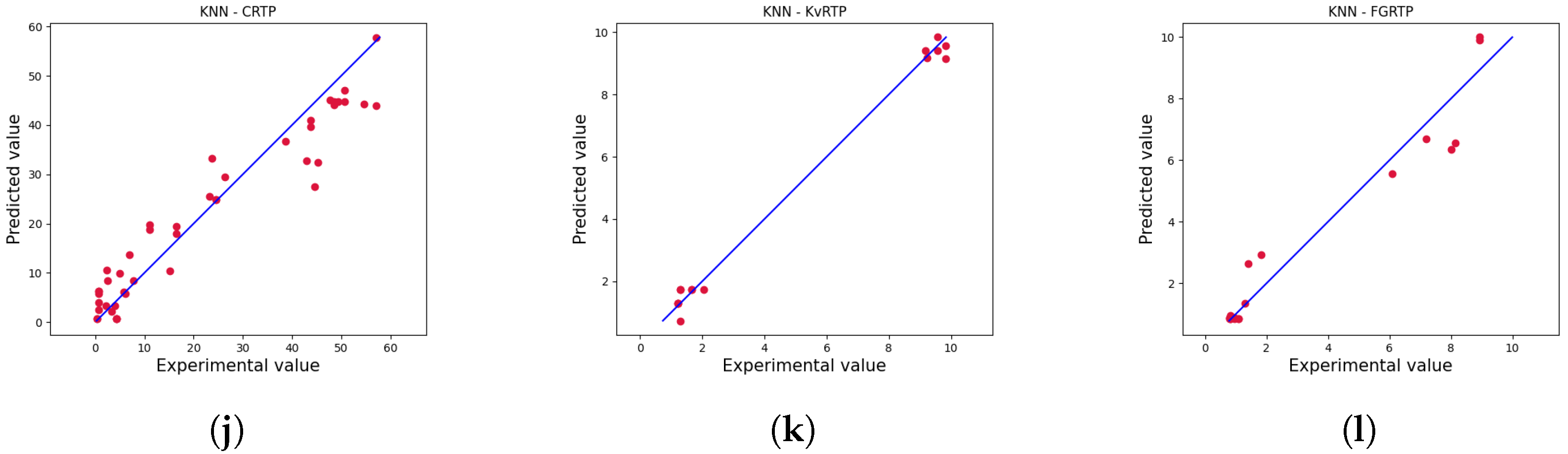
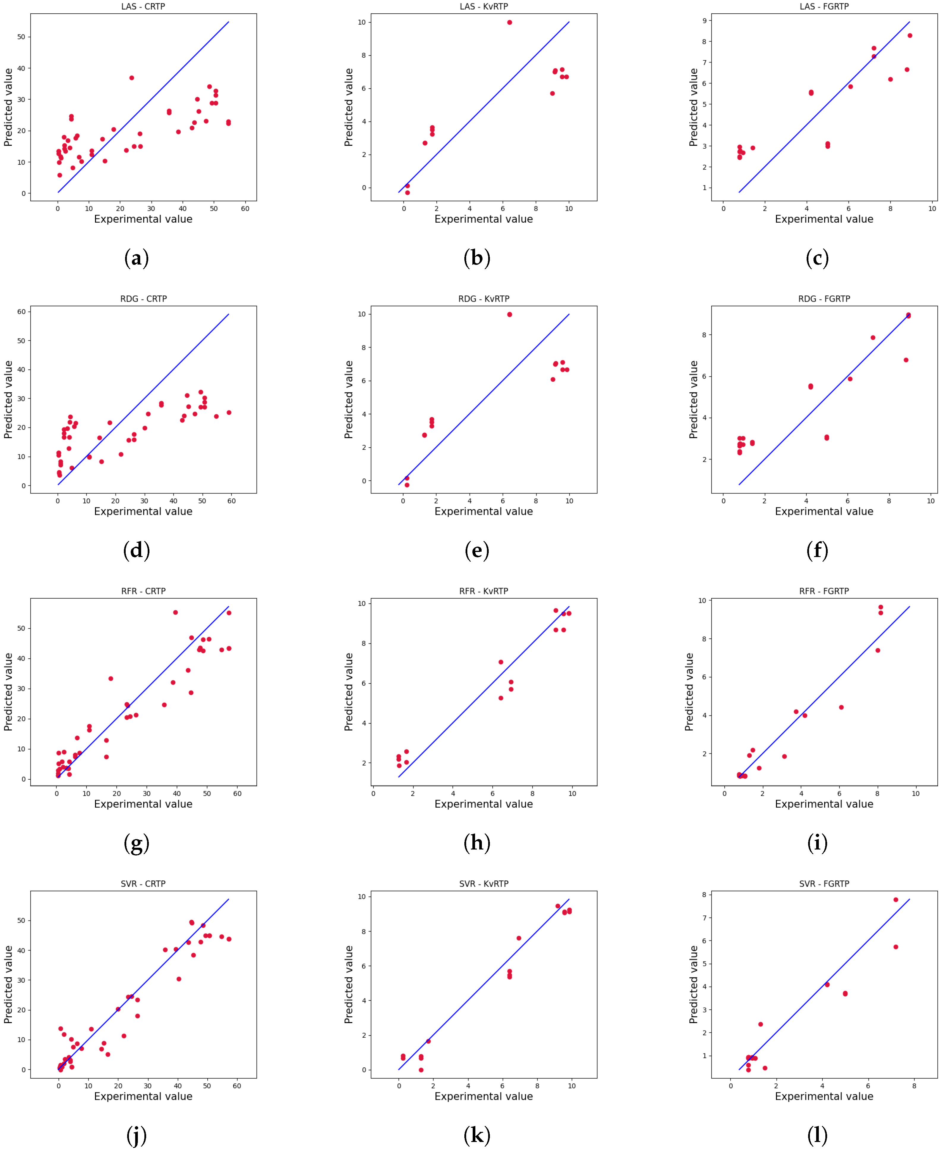
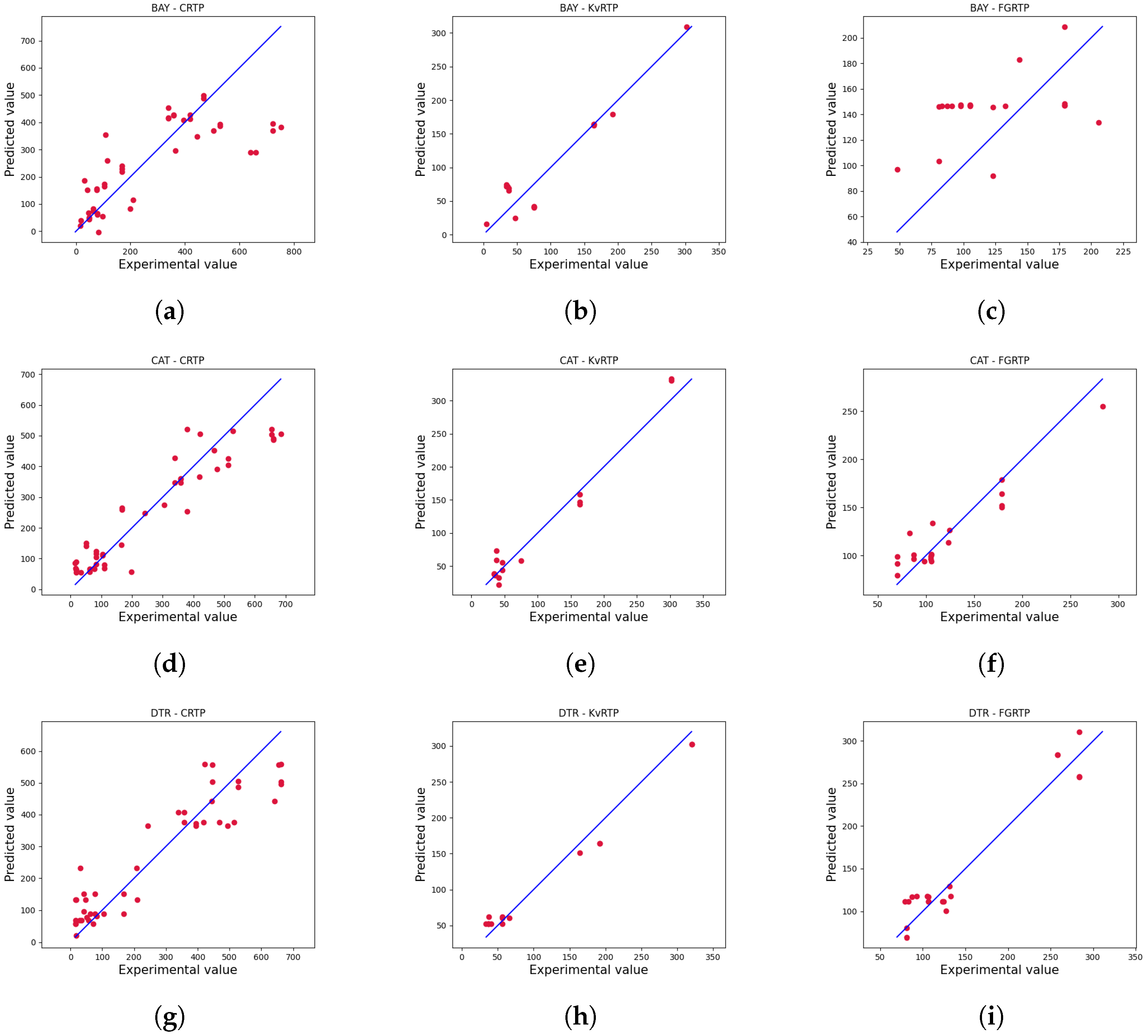
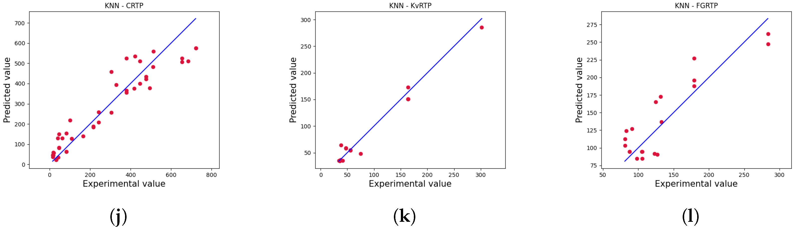
4.2. Numerical Results

The results regarding the performance of the models in the regression task are detailed in the following.

Table 3. RMSE summary statistics for the one hundred tests predicting E.

Model	Mean	Std Dev	Min.	1st Quartile	Median	3rd Quartile	Max
BAY	16.2405	3.2572	9.4879	14.0424	15.8779	18.3325	24.2133
RDG	16.2256	3.4534	9.0721	13.8824	16.0427	18.6324	25.0582
LAS	16.1670	3.2741	8.9366	14.1336	15.6067	18.0086	23.7556
DTR	14.8774	4.3100	7.6346	12.0422	14.4884	16.7512	27.0928
SVR	11.7524	5.0485	2.9113	7.6782	12.4260	15.4035	21.4587
RFR	9.8297	3.6813	3.6341	6.8087	8.6466	12.3373	19.6891
KNN	9.8020	4.1159	3.7364	6.6482	9.3383	11.9770	23.3197
CAT	9.4446	3.3558	3.0735	7.2028	8.8084	11.7664	18.1977

presents the summary statistics of the Root Mean Squared Error (RMSE) for the prediction of E. The results show that BAY, RDG, and LAS achieved similar performances, as evidenced by the slight differences in the summary statistics and the boxplots depicted in Figure 8b. Among them, the LAS had the best performance since it achieved the lowest mean value of the RMSE. However, such a result is still unsatisfactory since the mean RMSE value was higher than 10% of the dataset’s maximum E value. The DTR and SVR performed a little better than the linear models but still not in a way to be considered satisfactory. Alternatively, the RFR, KNN, and CAT stood out from the linear models, achieving mean RMSE values of close to half of the values achieved by the linear models. Despite the similar performances, the statistics show that the latter achieved more consistent results with a narrower RMSE distribution, as shown in Figure 8b. Therefore, the boosting model had the best performance in the elastic modulus prediction task. On the other hand, the results for the $\sigma$ prediction are summarized in

Table 4. RMSE summary statistics for the one hundred tests predicting $\sigma$.

Model	Mean	Std Dev	Min.	1st Quartile	Median	3rd Quartile	Max
BAY	159.7859	24.6198	131.2626	143.6800	156.5881	166.6547	258.1069
RDG	159.4300	25.2739	128.5327	143.7674	155.4155	167.4714	258.7639
LAS	159.3340	25.2431	129.0285	143.4035	155.3209	166.2181	258.7624
DTR	152.2683	45.3625	76.5504	115.0226	150.2737	170.3594	289.0174
SVR	142.2886	43.2337	71.5865	115.0798	144.5133	164.2971	258.5963
KNN	121.4163	42.1382	53.4138	91.3910	111.6907	141.3862	251.2954
CAT	114.4038	32.6867	54.2600	91.3665	109.3586	139.4164	197.8857
RFR	113.1730	36.8256	52.8864	84.8905	107.1129	136.4452	209.2337

. Similarly to what happened for E, the linear models were the ones with the worst performance. The mean RMSE values achieved by BAY, RDG, and LAS are almost equal to 20% of the maximum $\sigma$ value in the dataset. In this situation, CAT and RFR performed considerably better than the linear models, DTR, SVR, and KNN. Despite the lower mean RMSE for RFR, CAT outperformed the former with a narrower distribution; see Figure 8a.

As previously discussed, building a model for predicting the mechanical properties of additively manufactured composites from printing properties is challenging. Therefore, it could be expected that linear models (BAY, RDG, and LAS) would not achieve adequate performances since they cannot capture the nonlinear relationships between the input variables (printing properties) and the mechanical properties. On the other hand, models such as SVR and DTR can better deal with nonlinearities between input and output variables, thus performing better than linear regression models, as shown by the metrics reported. The RFR and CAT models performed even better because, in addition to being able to capture nonlinear relationships, they are an ensemble of decision tree models. Ensembles generally reduce the chance of overfitting and generate more robust predictions than single models. KNN also performed well, given its ability to capture nonlinearities and the fact that it is an algorithm that tends to produce good models when trained with small databases.

4.3. Computational Performance

The models’ computational performance results are disclosed in

Table 5. Computational performances of the models when predicting E and $\sigma$.

Target	Model	Prediction Time (ms)	Model Size (kB)
E	BAY	0.2464 ± 0.0655	1.8690 ± 0.0000
E	RDG	0.2571 ± 0.1237	1.0540 ± 0.0000
E	LAS	0.3108 ± 0.2160	1.1542 ± 0.0004
E	DTR	0.2475 ± 0.0485	2.6079 ± 0.0808
E	SVR	0.3114 ± 0.0791	9.8657 ± 0.3070
E	RFR	2.5034 ± 0.8491	323.2075 ± 107.4422
E	KNN	13.2900 ± 0.3737	12.1362 ± 0.0033
E	CAT	1.0333 ± 0.3281	213.9868 ± 114.2556
$\sigma$	BAY	0.2542 ± 0.0797	1.8690 ± 0.0000
$\sigma$	RDG	0.2395 ± 0.0714	1.0540 ± 0.0000
$\sigma$	LAS	0.2494 ± 0.0535	1.1542 ± 0.0004
$\sigma$	DTR	0.2458 ± 0.0525	2.5439 ± 0.1393
$\sigma$	SVR	0.3184 ± 0.0753	10.5268 ± 0.0322
$\sigma$	KNN	13.3308 ± 0.3256	12.1356 ± 0.0024
$\sigma$	CAT	0.9430 ± 0.2397	198.7430 ± 102.1022
$\sigma$	RFR	2.8011 ± 0.9439	349.6818 ± 88.7123

. The prediction time refers to the interval when the model calculates the value of the target variable based on the manufacturing properties. At the same time, the size represents the amount of space that the model occupies in a storage disk. One can notice that both metrics follow the same pattern independently of the target variable. Despite their poor performance discussed previously, the linear models have shown to be considerably faster and smaller than the KNN and CAT. The tree-based model can also be considered fast as it can make a prediction in less than 1 ms, despite being one of the largest models. Moreover, despite being able to make a prediction in more than 10 ms, the k-neighbor model is at least ten-fold smaller than the ensemble. Therefore, there is a clear size versus prediction time tradeoff between the CAT and KNN, the models with the best regression performance.

In summary, the linear models can serve as a baseline and have proven inadequate for predicting the mechanical properties of AM composite parts despite having the lowest computational complexity. On the other hand, both the KNN and CAT presented satisfactory regression performances, thus being suitable for performing the task at hand. The goal of assessing metrics like size and prediction time is to evaluate the model with the best balance between the regression and computational performance. In this context, the size versus time tradeoff between the tree-based and the instance-based models makes the analysis difficult. However, in assuming that the predictive model will not be embedded in a device with restricted hardware, the prediction time can be used as the first criterion to define the more balanced candidate. In this sense, the CAT can be considered the most suitable solution to use as a predictive model for estimating the mechanical properties of AM composite parts based on their printing variables.

4.4. Detailed Results

In addition to presenting a performance for grouped data, an in-depth comparison between the models’ predictions and experimental values for the elastic modulus separated for each type of fiber reinforcement is shown in Figure 9 and Figure 10 and

Table 6. Detailed results for the prediction of E.

Fiber Type	Metric	SVR	DTR	RFR	CAT	KNN	RDG	LAS	BAY
	r	0.5835	0.6059	0.8062	0.8075	0.7972	0.3697	0.3473	0.3585
CRTP	$R^2$	0.3404	0.3672	0.6500	0.6521	0.6355	0.1367	0.1206	0.1285
	Student’s t-test	-	-	Ok	Ok	-	-	-	-
	r	−0.0075	0.0218	0.1100	0.1091	−0.0849	0.0250	−0.0119	−0.0370
FGRTP	$R^2$	0.0001	0.3672	0.6500	0.6521	0.6355	0.1367	0.1206	0.1285
	Student’s t-test	-	-	Ok	Ok	-	-	-	-
	r	0.5240	0.4342	0.5789	0.6695	0.7870	0.2731	0.2546	0.2715
KvRTP	$R^2$	0.2746	0.1885	0.3351	0.4482	0.6193	0.0746	0.0648	0.0737
	Student’s t-test	-	-	-	-	Ok	-	-	-

. The plots depicted in the figures show the predicted values on the vertical and the experimental values on the horizontal axis. The table displays several statistics, including the Pearson correlation coefficient (r) [73], the coefficient of determination ($R^2$) [74], and the result of a Student’s t-test [75] with the null hypothesis stating that there is no significant difference between the predicted and experimental values (with 0.05 significance level). The metrics and the adjustments between predicted and experimental values for the carbon fiber (CRTP) highlight the poor performance of the linear models (RDG and LAS) and the Bayesian model. For all of them, the r was inferior to 0.40, the ($R^2$) lower than 0.20, and the null hypothesis was rejected in the Student’s t-test. The results for SVR and DTR highlight their average performance, while the KNN, RFR, and CAT stand out with acceptable correlation metrics. However, since the null hypothesis was rejected in the Student’s t-test for KNN, only the tree-based models can be considered sufficiently robust for performing the task. The same pattern is observed for the fiberglass, where RFR and CAT stood out from the other models. On the other hand, for the kevlar fiber only the KNN passed the Student’s t-test and achieved good correlation metrics.

On the other hand, the detailed results for the tensile strength problem are shown in Figure 11 and Figure 12,

Table 7. Detailed results for the prediction of $\sigma$.

Fiber Type	Metric	SVR	DTR	RFR	CAT	KNN	RDG	LAS	BAY
	r	0.6819	−0.0686	−0.1237	−0.0471	-0.1073	−0.0528	−0.0528	−0.0408
CRTP	$R^2$	0.4649	0.0047	0.0153	0.0022	0.0115	0.0028	0.0028	0.0017
	Student’s t-test	-	Ok	Ok	Ok	-	-	-	-
	r	0.0846	−0.0206	0.0897	0.0886	−0.0013	−0.0325	-0.0212	-0.0450
FGRTP	$R^2$	0.0072	0.0004	0.0080	0.0078	0.0000	0.0011	0.0004	0.0020
	Student’s t-test	-	-	-	-	-	-	-	-
	r	0.8297	0.7266	0.8532	0.8146	0.7031	0.8235	0.8235	0.8215
KvRTP	$R^2$	0.6884	0.5279	0.7279	0.6635	0.4944	0.6782	0.6782	0.6749
	Student’s t-test	-	-	-	-	-	-	-	-

. Analyzing the results for the CRTP, one can see that all of the models, with the exception of the SVR, achieved a poor performance. The support vector was the only one to achieve r ≫ 0.5 and a reasonable ($R^2$) despite not passing the Student’s t-test. The same bad performance is also observed for the FGRTP case. None of the models passed the Student’s t-test and the coefficients are far from values representing a good prediction performance. On the other hand, for the KvRTP, most of the models achieved good metrics, and the plots highlight a reasonable correlation, but none of them were able to pass the Student’s t-test.

Unlike the commonly accepted ROM, the results here show no linear dependence. The nonlinearities induced by factors chosen by a designer, such as matrix filling or involuntary ones intrinsic to the fabrication process, such as porosity [37] or even the effect of the sample shape defined by the standard used on the test or the lack of adhesion between fiber and matrix [4] might not be well represented by the ML linear models. Finding the right combination of printing parameters will give the appropriate strength and stiffness needed for a part while maintaining geometry and density within requirements. Additionally, it helps maintain dimensional tolerances, which is crucial for applications that require high precision, reduced printing time, and material consumption, which translates into lower costs and Waste Reduction by minimizing waste produced during manufacturing.

5. Conclusions

Predicting mechanical properties for composite materials fabricated via AM is challenging. Currently, the available predictive models do not include all the variables and require highly skilled users with vast knowledge of composite material’s mechanical behavior and advanced numerical modeling skills. This work evaluated different supervised learning models in order to check the suitability of employing ML for automatically predicting the mechanical properties of AM composite specimens. The predictive models were trained to estimate the strength and elasticity of AM composite reinforced with fibers like carbon, Kevlar, and fiberglass. To do so, a diverse dataset was constructed based on data published in the literature.

The results obtained for the ML model, CAT, and the suitability of the proposed modeling workflow for obtaining a predictive model are capable of estimating, with reasonable performance, the mechanical properties of AM composite specimens. The best overall performance was achieved by the CAT and KNN models, with the first standing out since it required less time to estimate the mechanical properties of a given sample. The model takes around 1 ms to make a prediction while achieving relatively low error rates of 9.4446 and 113.1730 for E and $\sigma$ prediction, respectively.

Despite the achievements reported, there is room for improvement in future work. The results are limited to the parameters and materials studied (nylon matrix and carbon, Kevlar, and fiberglass fibers). With this in mind, no applications with cellular structures such as gyroid honeycombs, foams (open- and closed-cell), lattices (grids, octets, face cubic centered, body cubic centered, or X-shaped), and others cannot be considered to be used in conjunction with the results found here. Other parameters, which users can tweak in different systems, such as printing and feeding speed, cannot be included here as the Eiger^® software does not allow modification. Moreover, although the dataset comprises several samples from different sources, it is still a small dataset from the ML perspective. For this reason, data augmentation techniques can be explored in future work. To improve robustness in prediction, Physics-informed Neural Networks (PINNs) [76] can be used. For this, data could be organized in feature ranges to observe holes within that can be filled through simulation, i.e., with the finite element method. Such numerical data can be fed to an ML algorithm in conjunction with experimental data.

References

1. Chacón, J.; Caminero, M.A.; García-Plaza, E.; Núnez, P.J. Additive manufacturing of PLA structures using fused deposition modelling: Effect of process parameters on mechanical properties and their optimal selection. Mater. Des. 2017, 124, 143–157. [Google Scholar] [CrossRef]
2. Ngo, T.D.; Kashani, A.; Imbalzano, G.; Nguyen, K.T.; Hui, D. Additive manufacturing (3D printing): A review of materials, methods, applications and challenges. Compos. Part B Eng. 2018, 143, 172–196. [Google Scholar] [CrossRef]
3. Torries, B.; Shamsaei, N. Fatigue behavior and modeling of additively manufactured Ti-6Al-4V including interlayer time interval effects. Jom 2017, 69, 2698–2705. [Google Scholar] [CrossRef]
4. Díaz, J.G.; Pertúz-Comas, A.D.; González-Estrada, O.A. Mechanical properties for long fibre reinforced fused deposition manufactured composites. Compos. Part B Eng. 2021, 211, 108657. [Google Scholar] [CrossRef]
5. Mark, G.T.; Gozdz, A.S. Three Dimensional Printer with Composite Filament Fabrication. US Patent 10,099,427, 16 October 2018. [Google Scholar]
6. Becerra, J.L.; Díaz-Rodríguez, J.G.; González-Estrada, O.A. Daño en partes de manufactura aditiva reforzadas por fibras continuas. Rev. UIS Ing. 2020, 19, 161–176. [Google Scholar] [CrossRef]
7. Hassani-Gangaraj, S.; Moridi, A.; Guagliano, M.; Ghidini, A.; Boniardi, M. The effect of nitriding, severe shot peening and their combination on the fatigue behavior and micro-structure of a low-alloy steel. Int. J. Fatigue 2014, 62, 67–76. [Google Scholar] [CrossRef]
8. Parrado-Agudelo, J.Z.; Narváez-Tovar, C. Mechanical characterization of polylactic acid, polycaprolactone and Lay-Fomm 40 parts manufactured by fused deposition modeling, as a function of the printing parameters. Iteckne 2019, 16, 111–117. [Google Scholar] [CrossRef]
9. Uribe-Lam, E.; Treviño-Quintanilla, C.D.; Cuan-Urquizo, E.; Olvera-Silva, O. Use of additive manufacturing for the fabrication of cellular and lattice materials: A review. Mater. Manuf. Process. 2020, 36, 257–280. [Google Scholar] [CrossRef]
10. León-Becerra, J.S.; González-Estrada, O.A.; Pinto-Hernández, W. Mechanical characterization of additive manufacturing composite parts. Respuestas 2020, 25, 109–116. [Google Scholar] [CrossRef]
11. Wickramasinghe, S.; Do, T.; Tran, P. FDM-Based 3D printing of polymer and associated composite: A review on mechanical properties, defects and treatments. Polymers 2020, 12, 1529. [Google Scholar] [CrossRef]
12. Kabir, S.M.F.; Mathur, K.; Seyam, A.F.M. A critical review on 3D printed continuous fiber-reinforced composites: History, mechanism, materials and properties. Compos. Struct. 2020, 232, 111476. [Google Scholar] [CrossRef]
13. Goh, G.D.; Dikshit, V.; Nagalingam, A.P.; Goh, G.L.; Agarwala, S.; Sing, S.L.; Wei, J.; Yeong, W.Y. Characterization of mechanical properties and fracture mode of additively manufactured carbon fiber and glass fiber reinforced thermoplastics. Mater. Des. 2018, 137, 79–89. [Google Scholar] [CrossRef]
14. Díaz-Rodríguez, J.G.; Pertúz-Comas, A.D.; Ariza-González, C.J.; Garcia-López, D.D.; Pinto-Hernández, W. Monotonic crack propagation in a notched polymer matrix composite reinforced with continuous fiber and printed by material extrusion. Prog. Addit. Manuf. 2023, 8, 733–744. [Google Scholar] [CrossRef]
15. Pertúz-Comas, A.D.; Díaz, J.G.; Meneses-Duran, O.J.; Niño-Álvarez, N.Y.; León-Becerra, J. Flexural Fatigue in a Polymer Matrix Composite Material Reinforced with Continuous Kevlar Fibers Fabricated by Additive Manufacturing. Polymers 2022, 14, 3586. [Google Scholar] [CrossRef] [PubMed]
16. ASTM638; Standard Test Method for Tensile Properties of Plastics on Mechanical Properties, Defects and Treatments. ASTM International: West Conshohocken, PA, USA, 2014. [CrossRef]
17. ASTM3039; Standard Test Method for Tensile Properties of Polymer Matrix Composite Materials. ASTM International: West Conshohocken, PA, USA, 2014. [CrossRef]
18. Dutra, T.A.; Ferreira, R.T.L.; Resende, H.B.; Guimarães, A. Mechanical characterization and asymptotic homogenization of 3D-printed continuous carbon fiber-reinforced thermoplastic. J. Braz. Soc. Mech. Sci. Eng. 2019, 41, 133. [Google Scholar] [CrossRef]
19. Melenka, G.W.; Cheung, B.K.O.; Schofield, J.S.; Dawson, M.R.; Carey, J.P. Evaluation and prediction of the tensile properties of continuous fiber-reinforced 3D printed structures. Compos. Struct. 2016, 153, 866–875. [Google Scholar] [CrossRef]
20. Ansari, A.A.; Kamil, M. Performance Study of 3D Printed Continuous Fiber-Reinforced Polymxer Composites Using Taguchi Method. J. Mater. Eng. Perform. 2022, 32, 9892–9906. [Google Scholar] [CrossRef]
21. Lupone, F.; Padovano, E.; Venezia, C.; Badini, C. Experimental Characterization and Modeling of 3D Printed Continuous Carbon Fibers Composites with Different Fiber Orientation Produced by FFF Process. Polymers 2022, 14, 26. [Google Scholar] [CrossRef]
22. Azarov, A.V.; Antonov, F.K.; Golubev, M.V.; Khaziev, A.R.; Ushanov, S.A. Composite 3D printing for the small size unmanned aerial vehicle structure. Compos. Part B Eng. 2019, 169, 157–163. [Google Scholar] [CrossRef]
23. Swolfs, Y.; Pinho, S.T. 3D printed continuous fibre-reinforced composites: Bio-inspired microstructures for improving the translaminar fracture toughness. Compos. Sci. Technol. 2019, 182, 107731. [Google Scholar] [CrossRef]
24. León-Becerra, J.; Hidalgo-Salazar, M.; González-Estrada, O.A. Progressive damage analysis of carbon fiber-reinforced additive manufacturing composites. Int. J. Adv. Manuf. Technol. 2023, 126, 2617–2631. [Google Scholar] [CrossRef]
25. Gibson, L.J.; Ashby, M.F. Cellular Solids. Structure and Properties, 2nd ed.; Cambridge University Press: Cambridge, UK, 2014. [Google Scholar] [CrossRef]
26. León-Becerra, J.; González-Estrada, O.A.; Quiroga, J. Effect of Relative Density in In-Plane Mechanical Properties of Common 3D-Printed Polylactic Acid Lattice Structures. ACS Omega 2021, 6, 29830–29838. [Google Scholar] [CrossRef]
27. Barbero, E.J. Finite Element Analysis of Composite Materials Using ANSYS, 2nd ed.; CRC Press: Boca Raton, FL, USA, 2013. [Google Scholar]
28. Ng, W.L.; Goh, G.L.; Goh, G.D.; Ten, J.S.J.; Yeong, W.Y. Progress and Opportunities for Machine Learning in Materials and Processes of Additive Manufacturing. Adv. Mater. 2024, 2310006. [Google Scholar] [CrossRef]
29. Zhu, S.P.; Wang, L.; Luo, C.; Correia, J.A.F.O.; Jesus, A.M.P.D.; Berto, F. Physics-informed machine learning and its structural integrity applications: State of the art. Philos. Trans. R. Soc. A 2024, 381, 20220406. [Google Scholar] [CrossRef]
30. Gaikwad, A.; Giera, B.; Guss, G.M.; Forien, J.B.; Matthews, M.J.; Rao, P. Heterogeneous sensing and scientific machine learning for quality assurance in laser powder bed fusion—A single-track study. Addit. Manuf. 2020, 36, 101659. [Google Scholar] [CrossRef]
31. Tavares, T.B.; Finamor, F.P.; de Sousa Zorzi, J.C. Mechanical properties prediction of dual phase steels using machine learning. Rev. Tecnol. Em Metal. Mater. E Mineração 2022, 19, e2595. [Google Scholar] [CrossRef]
32. Jin, Z.; Zhang, Z.; Demir, K.; Gu, G.X. Machine Learning for Advanced Additive Manufacturing. Matter 2020, 3, 1541–1556. [Google Scholar] [CrossRef]
33. Liu, X.; Tian, S.; Tao, F.; Yu, W. A review of artificial neural networks in the constitutive modeling of composite materials. Compos. Part B Eng. 2021, 224, 109152. [Google Scholar] [CrossRef]
34. Okafor, C.E.; Iweriolor, S.; Ani, O.I.; Ahmad, S.; Mehfuz, S.; Ekwueme, G.O.; Chukwumuanya, O.E.; Abonyi, S.E.; Ekengwu, I.E.; Chikelu, O.P. Advances in machine learning-aided design of reinforced polymer composite and hybrid material systems. Hybrid Adv. 2023, 2, 100026. [Google Scholar] [CrossRef]
35. Zhang, J.; Wang, P.; Gao, R.X. Deep learning-based tensile strength prediction in fused deposition modeling. Comput. Ind. 2019, 107, 11–21. [Google Scholar] [CrossRef]
36. Leon-Becerra, J.; González-Estrada, O.A.; Sánchez-Acevedo, H. Comparison of Models to Predict Mechanical Properties of FR-AM Composites and a Fractographical Study. Polymers 2022, 14, 3546. [Google Scholar] [CrossRef]
37. Rodríguez, J.F.; Thomas, J.P.; Renaud, J.E. Mechanical behavior of ABS fused deposition materials modeling. Rapid Prototyp. J. 2003, 9, 219–230. [Google Scholar] [CrossRef]
38. Papon, E.A.; Haque, A. Tensile properties, void contents, dispersion and fracture behaviour of 3D printed carbon nanofiber reinforced composites. J. Reinf. Plast. Compos. 2018, 37, 381–395. [Google Scholar] [CrossRef]
39. Boyd, S.; Vandenberghe, L. Introduction to Applied Linear Algebra: Vectors, Matrices, and Least Squares; Cambridge University Press: Cambridge, UK, 2018. [Google Scholar]
40. Brunton, S.L.; Kutz, J.N. Data-Driven Science and Engineering—Machine Learning, Dynamical Systems, and Control; Cambridge University Press: Cambridge, UK, 2019. [Google Scholar]
41. Hancock, J.T.; Khoshgoftaar, T.M. CatBoost for big data: An interdisciplinary review. J. Big Data 2020, 7, 94. [Google Scholar] [CrossRef]
42. Dorogush, A.V.; Ershov, V.; Gulin, A. CatBoost: Gradient boosting with categorical features support. arXiv 2018, arXiv:1810.11363. [Google Scholar]
43. Kramer, O. K-Nearest Neighbors; Springer: Berlin/Heidelberg, Germany, 2013. [Google Scholar] [CrossRef]
44. Blok, L.; Longana, M.; Yu, H.; Woods, B. An investigation into 3D printing of fibre reinforced thermoplastic composites. Addit. Manuf. 2018, 22, 176–186. [Google Scholar] [CrossRef]
45. Klift, F.V.D.; Koga, Y.; Todoroki, A.; Ueda, M.; Hirano, Y.; Matsuzaki, R. 3D Printing of Continuous Carbon Fibre Reinforced Thermo-Plastic (CFRTP) Tensile Test Specimens. Open J. Compos. Mater. 2016, 6, 18–27. [Google Scholar] [CrossRef]
46. Dickson, A.N.; Ross, K.A.; Dowling, D.P. Additive manufacturing of woven carbon fibre polymer composites. Compos. Struct. 2018, 206, 637–643. [Google Scholar] [CrossRef]
47. Justo, J.; Távara, L.; García-Guzmán, L.; París, F. Characterization of 3D printed long fibre reinforced composites. Compos. Struct. 2018, 185, 537–548. [Google Scholar] [CrossRef]
48. Abadi, H.A.; Thai, H.T.; Paton-Cole, V.; Patel, V. Elastic properties of 3D printed fibre-reinforced structures. Compos. Struct. 2018, 193, 8–18. [Google Scholar] [CrossRef]
49. Imeri, A.; Fidan, I.; Allen, M.; Wilson, D.A.; Canfield, S. Fatigue analysis of the fiber reinforced additively manufactured objects. Int. J. Adv. Manuf. Technol. 2018, 98, 2717–2724. [Google Scholar] [CrossRef]
50. Mohammadizadeh, M.; Imeri, A.; Fidan, I.; Elkelany, M. 3D printed fiber reinforced polymer composites - Structural analysis. Compos. Part B Eng. 2019, 175, 107112. [Google Scholar] [CrossRef]
51. Todoroki, A.; Oasada, T.; Mizutani, Y.; Suzuki, Y.; Ueda, M.; Matsuzaki, R.; Hirano, Y. Tensile property evaluations of 3D printed continuous carbon fiber reinforced thermoplastic composites. Adv. Compos. Mater. 2020, 29, 147–162. [Google Scholar] [CrossRef]
52. Araya-Calvo, M.; López-Gómez, I.; Chamberlain-Simon, N.; León-Salazar, J.L.; Guillén-Girón, T.; Corrales-Cordero, J.S.; Sánchez-Brenes, O. Evaluation of compressive and flexural properties of continuous fiber fabrication additive manufacturing technology. Addit. Manuf. 2018, 22, 157–164. [Google Scholar] [CrossRef]
53. González-Estrada, O.A.; Pertuz, A.; Quiroga Mendez, J.E. Evaluation of tensile properties and damage of continuous fibre reinforced 3D-printed parts. Key Eng. Mater. 2018, 774, 161–166. [Google Scholar] [CrossRef]
54. Pertuz, A.D.; Díaz-Cardona, S.; González-Estrada, O.A. Static and fatigue behaviour of continuous fibre reinforced thermoplastic composites manufactured by fused deposition modelling technique. Int. J. Fatigue 2020, 130, 105275. [Google Scholar] [CrossRef]
55. Podda, F. Modellazione, Produzione e Testing di Materiali Compositi a Fibra Lunga Realizzati Mediante Additive Manufacturing = Modelling, Production and Testing of Long Fibre Composites via Additive Manufacturing. Ph.D. Thesis, Politecnico di Torino, Turin, Italy, 2018. [Google Scholar]
56. Agarwal, K.; Kuchipudi, S.K.; Girard, B.; Houser, M. Mechanical properties of fiber reinforced polymer composites: A comparative study of conventional and additive manufacturing methods. J. Compos. Mater. 2018, 52, 3173–3181. [Google Scholar] [CrossRef]
57. Mei, H.; Ali, Z.; Ali, I.; Cheng, L. Tailoring strength and modulus by 3D printing different continuous fibers and filled structures into composites. Adv. Compos. Hybrid Mater. 2019, 2, 312–319. [Google Scholar] [CrossRef]
58. Naranjo-Lozada, J.; Ahuett-Garza, H.; Orta-Castañón, P.; Verbeeten, W.M.; Sáiz-González, D. Tensile properties and failure behavior of chopped and continuous carbon fiber composites produced by additive manufacturing. Addit. Manuf. 2019, 26, 227–241. [Google Scholar] [CrossRef]
59. Pyl, L.; Kalteremidou, K.A.; Hemelrijck, D.V. Exploration of specimen geometry and tab configuration for tensile testing exploiting the potential of 3D printing freeform shape continuous carbon fibre-reinforced nylon matrix composites. Polym. Test. 2018, 71, 318–328. [Google Scholar] [CrossRef]
60. Saeed, K.; McIlhagger, A.; Harkin-Jones, E.; McGarrigle, C.; Dixon, D.; Shar, M.A.; McMillan, A.; Archer, E. Characterization of continuous carbon fibre reinforced 3D printed polymer composites with varying fibre volume fractions. Compos. Struct. 2022, 282, 115033. [Google Scholar] [CrossRef]
61. Tessarin, A.; Zaccariotto, M.; Galvanetto, U.; Stocchi, D. A multiscale numerical homogenization-based method for the prediction of elastic properties of components produced with the fused deposition modelling process. Results Eng. 2022, 14, 100409. [Google Scholar] [CrossRef]
62. Lawrence, B.D.; Coatney, M.D.; Phillips, F.; Henry, T.C.; Nikishkov, Y.; Makeev, A. Evaluation of the mechanical properties and performance cost of additively manufactured continuous glass and carbon fiber composites. Int. J. Adv. Manuf. Technol. 2022, 120, 1135–1147. [Google Scholar] [CrossRef]
63. Santos, J.D.; Fernández, A.; Ripoll, L.; Blanco, N. Experimental Characterization and Analysis of the In-Plane Elastic Properties and Interlaminar Fracture Toughness of a 3D-Printed Continuous Carbon Fiber-Reinforced Composite. Polymers 2022, 14, 506. [Google Scholar] [CrossRef] [PubMed]
64. Heitkamp, T.; Girnth, S.; Kuschmitz, S.; Klawitter, G.; Waldt, N.; Vietor, T. Continuous Fiber-Reinforced Material Extrusion with Hybrid Composites of Carbon and Aramid Fibers. Appl. Sci. 2022, 12, 8830. [Google Scholar] [CrossRef]
65. Bendine, K.; Gibhardt, D.; Fiedler, B.; Backs, A. Experimental characterization and mechanical behavior of 3D printed CFRP. Eur. J. Mech. A Solids 2022, 94, 104587. [Google Scholar] [CrossRef]
66. Ojha, K.K.; Gugliani, G.; Francis, V. Tensile properties and failure behaviour of continuous kevlar fibre reinforced composites fabricated by additive manufacturing process. Adv. Mater. Process. Technol. 2022, 10, 142–156. [Google Scholar] [CrossRef]
67. Ali, Z.; Yan, Y.; Mei, H.; Cheng, L.; Zhang, L. Effect of infill density, build direction and heat treatment on the tensile mechanical properties of 3D-printed carbon-fiber nylon composites. Compos. Struct. 2023, 304, 116370. [Google Scholar] [CrossRef]
68. Xiang, J.; Cheng, P.; Wang, K.; Wu, Y.; Rao, Y.; Peng, Y. Interlaminar and translaminar fracture toughness of 3D-printed continuous fiber reinforced composites: A review and prospect. Polym. Compos. 2023, 45, 3883–3900. [Google Scholar] [CrossRef]
69. Lee, G.W.; Kim, T.H.; Yun, J.H.; Kim, N.J.; Ahn, K.H.; Kang, M.S. Strength of Onyx-based composite 3D printing materials according to fiber reinforcement. Front. Mater. 2023, 10, 1183816. [Google Scholar] [CrossRef]
70. Moreno-Núñez, B.; Abarca-Vidal, C.; Treviño-Quintanilla, C.; Sánchez-Santana, U.; Cuan-Urquizo, E.; Uribe-Lam, E. Experimental Analysis of Fiber Reinforcement Rings’ Effect on Tensile and Flexural Properties of Onyx™–Kevlar® Composites Manufactured by Continuous Fiber Reinforcement. Polymers 2023, 15, 1252. [Google Scholar] [CrossRef]
71. Gljušćić, M.; Franulović, M.; Lanc, D.; Božić, Ž. Application of digital image correlation in behavior modelling of AM CFRTP composites. Eng. Fail. Anal. 2022, 136, 106133. [Google Scholar] [CrossRef]
72. Ali, M. PyCaret: An Open Source, Low-Code Machine Learning Library in Python; PyCaret Version 1.0.0; 2020. [Google Scholar]
73. Cohen, I.; Huang, Y.; Chen, J.; Benesty, J.; Benesty, J.; Chen, J.; Huang, Y.; Cohen, I. Pearson correlation coefficient. In Noise Reduction in Speech Processing; Springer: Berlin/Heidelberg, Germany, 2009; pp. 1–4. [Google Scholar]
74. Ozer, D.J. Correlation and the coefficient of determination. Psychol. Bull. 1985, 97, 307. [Google Scholar] [CrossRef]
75. Student. The probable error of a mean. In Biometrika; Oxford University Press: Oxford, UK, 1908; pp. 1–25. [Google Scholar]
76. Raissi, M.; Perdikaris, P.; Karniadakis, G. Physics-informed neural networks: A deep learning framework for solving forward and inverse problems involving nonlinear partial differential equations. J. Comput. Phys. 2019, 378, 686–707. [Google Scholar] [CrossRef]
Figure 1. Schematic of composite MEX printing. Adapted from [6].
Applsci 14 07009 g001
Figure 2. Options to configure a part for fiber layout and matrix filling, adapted from [14,15].
Applsci 14 07009 g002
Figure 3. Different RUCs for infill patterns and geometrical parameters: (a) square, (b) honeycomb, and (c) triangular.
Applsci 14 07009 g003
Figure 4. Elastic modulus as a function of thickness over length for three different infills. Adapted from [14].
Applsci 14 07009 g004
Figure 5. Normalized strength as predicted by the ROM. Adapted from [4].
Applsci 14 07009 g005
Figure 6. Machine learning modeling workflow.
Applsci 14 07009 g006
Figure 7. Target variable versus fiber volume fraction: (a) depicts the correlation between σ and V f , while (b) shows the correlation between E and V f .
Applsci 14 07009 g007
Figure 8. RMSE boxplots for (a) σ and (b) E.
Applsci 14 07009 g008
Figure 9. Comparison for predicted vs. experimental Elastic modulus, GPa, part 1. From the top to the bottom, the lines display the results for BAY, CAT, DTR, and KNN. From the left to the right, the columns display the results for CRTP, KvRTP, and FGRTP, respectively.
Applsci 14 07009 g009aApplsci 14 07009 g009b
Figure 10. Comparison for predicted vs. experimental Elastic modulus, GPa, part 2. From the top to the bottom, the lines display the results for LAS, RDG, RFR, and SVR. From the left to the right, the columns display the results for CRTP, KvRTP, and FGRTP, respectively.
Applsci 14 07009 g010
Figure 11. Predicted vs. experimental values for the Tensile strength, MPa, part 1. From the top to the bottom, the lines display the results for BAY, CAT, DTR, and KNN. From the left to the right, the columns display the results for CRTP, KvRTP, and FGRTP, respectively.
Applsci 14 07009 g011aApplsci 14 07009 g011b
Figure 12. Predicted vs. experimental values for the Tensile strength, MPa, part 2. From the top to the bottom, the lines display the results for LAS, RDG, RFR, and SVR. From the left to the right, the columns display the results for CRTP, KvRTP, and FGRTP, respectively.
Applsci 14 07009 g012