
Contact Force and Friction of Generally Layered Laminates with Residual Hygrothermal Stresses under Mode II In-Plane-Shear Delamination

Abstract
:1. Introduction
2. Theoretical Background
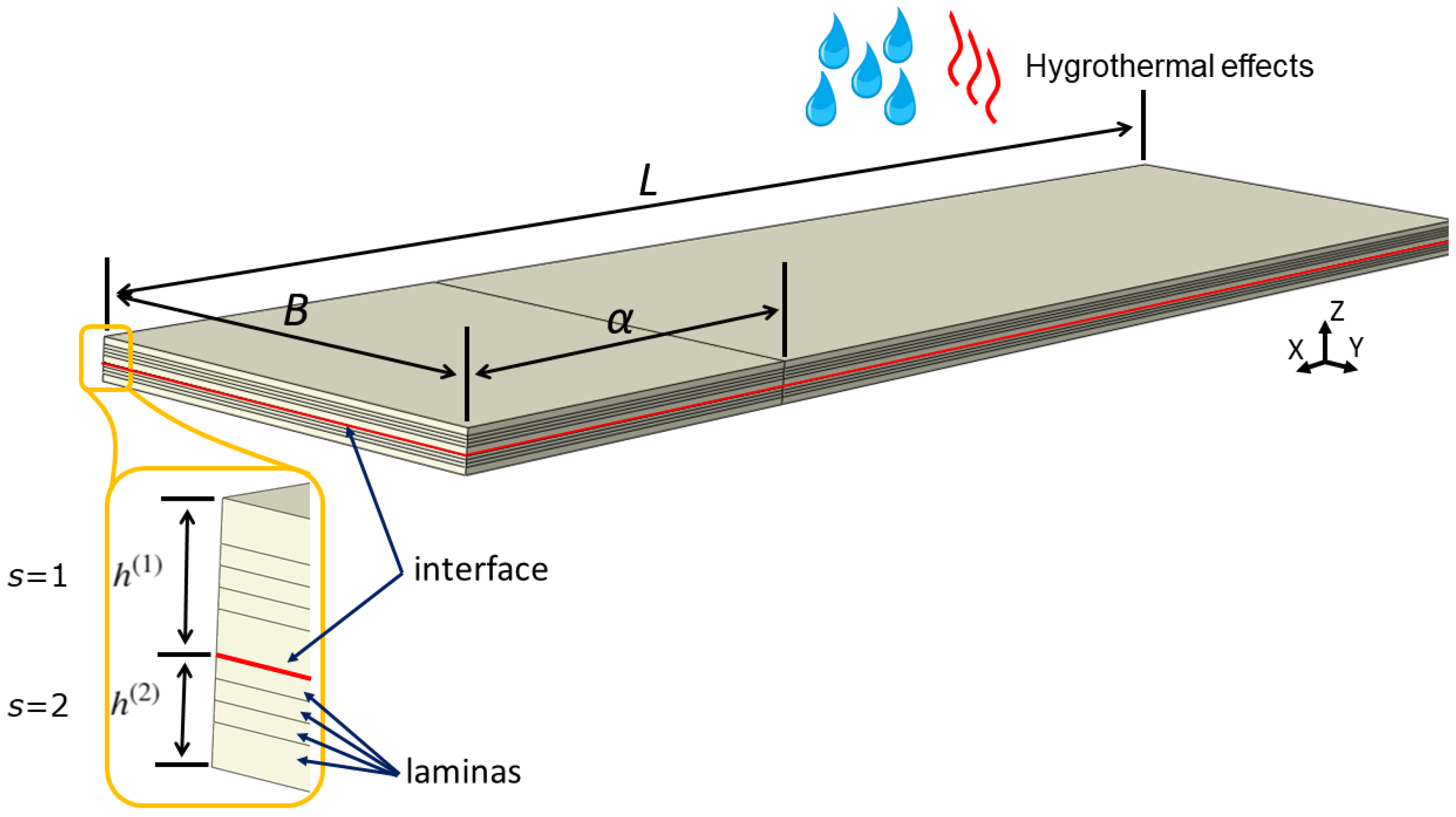
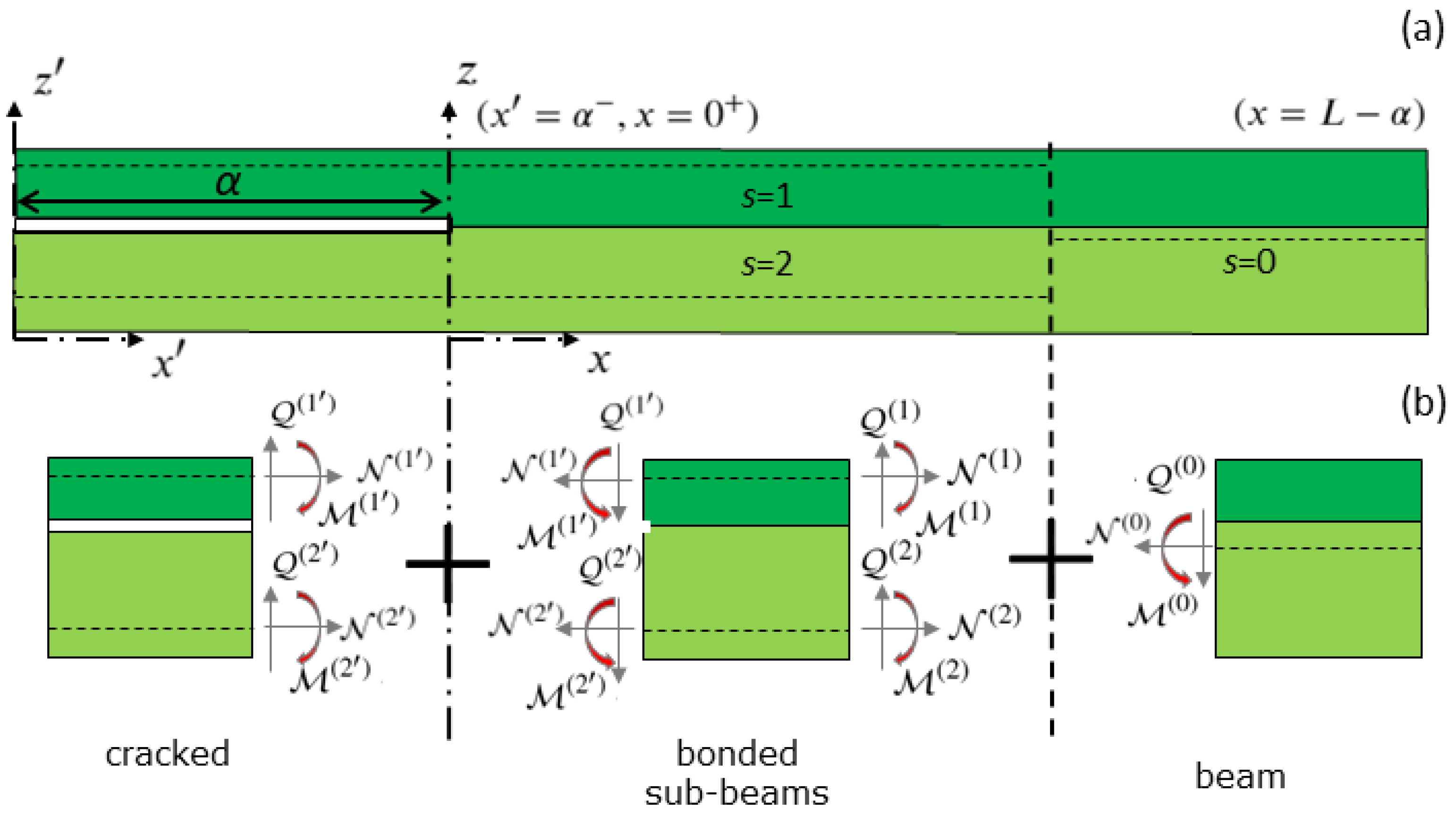
2.1. Problem Description
2.2. Static Equilibrium
2.3. Constitutive Equations
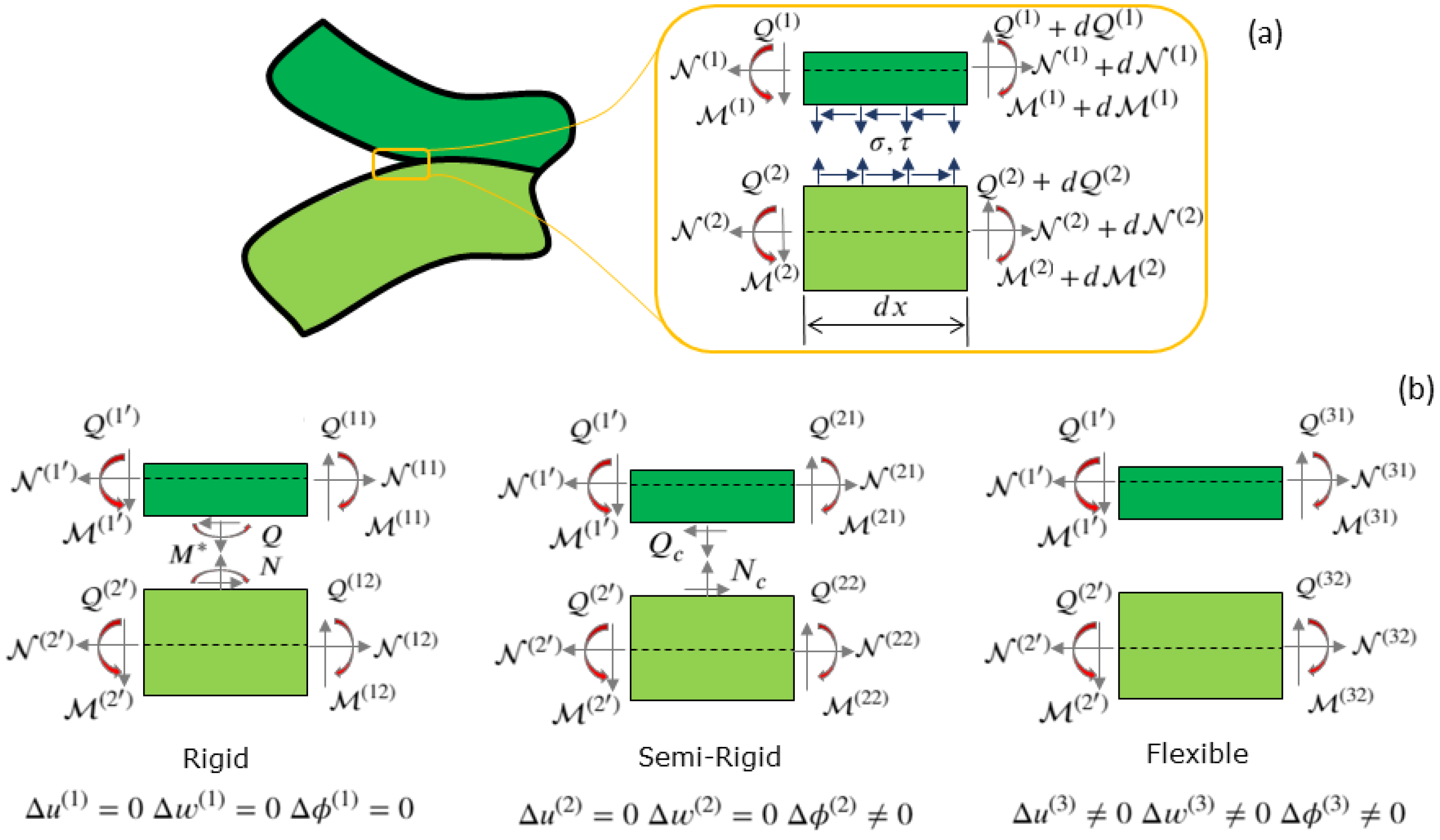
2.4. Analysis of the System of Two Sub-Beams
2.5. Continuity Conditions
2.5.1. Rigid Joint Model
2.5.2. Semi-Rigid Joint Model
2.5.3. Flexible Joint Model
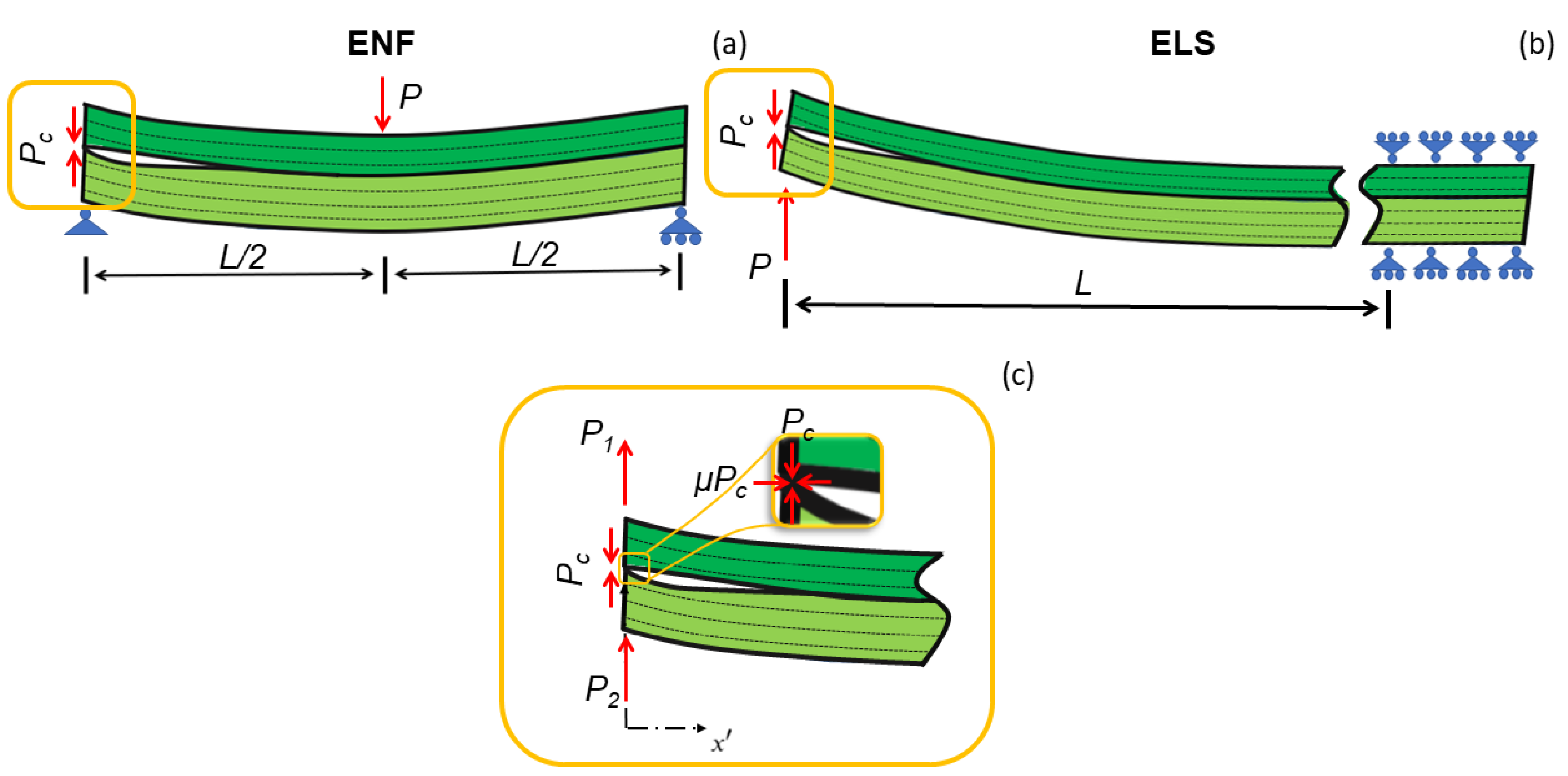
3. Mode II Delamination Tests
- ENF (, )
- ELS (, )
3.1. Contact Force between the Two Sub-Beams
3.2. Static Equilibrium
3.3. General Solution of Displacements and Rotation of the Cracked Part
3.4. Relative Displacement between the Two Sub-Beams
4. Case Study
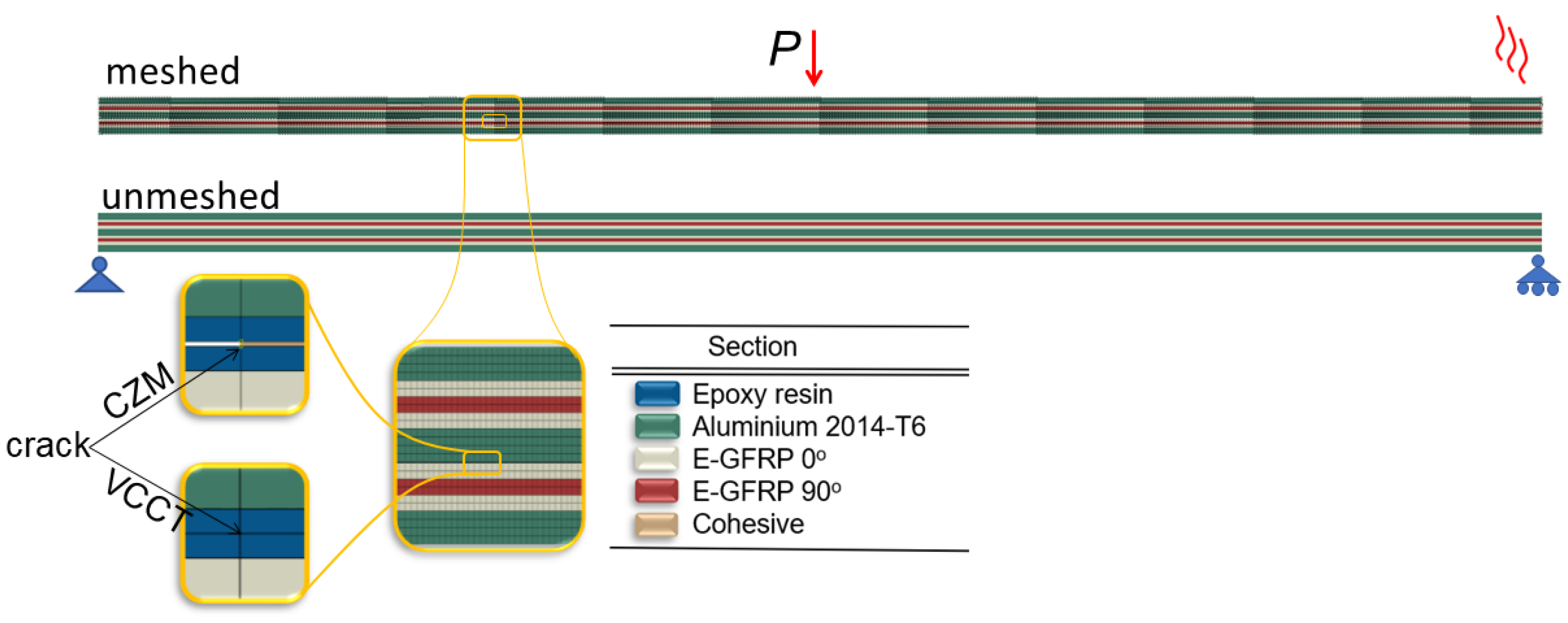
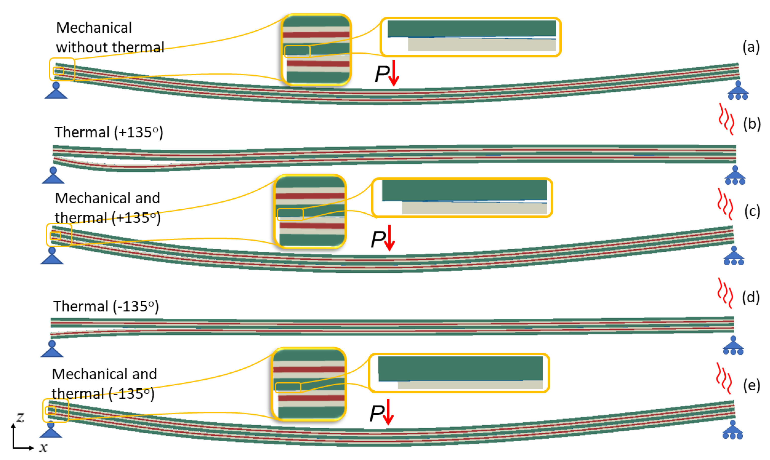
4.1. Description
4.2. Numerical Implementation
5. Results
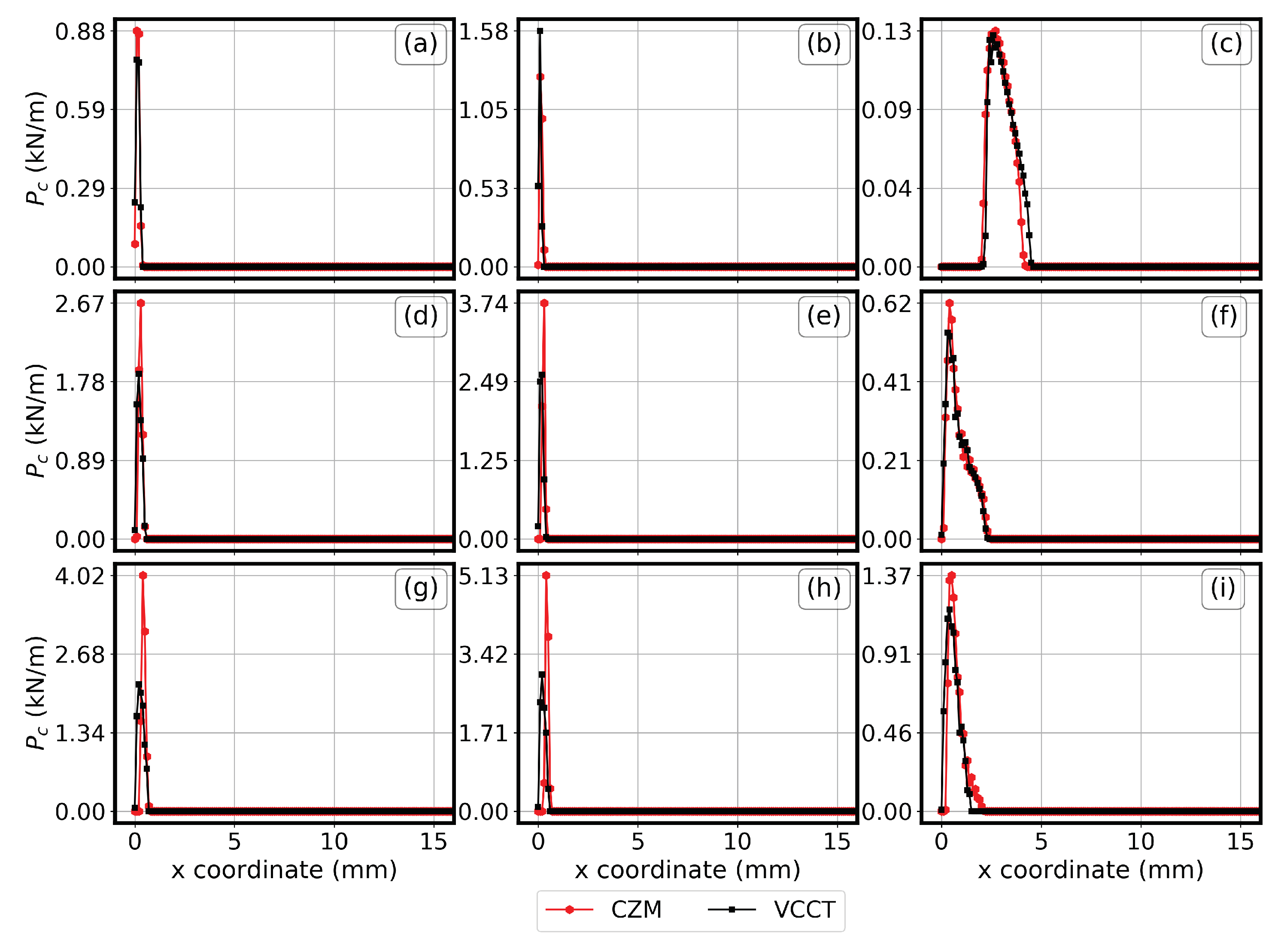
5.1. Contact Force
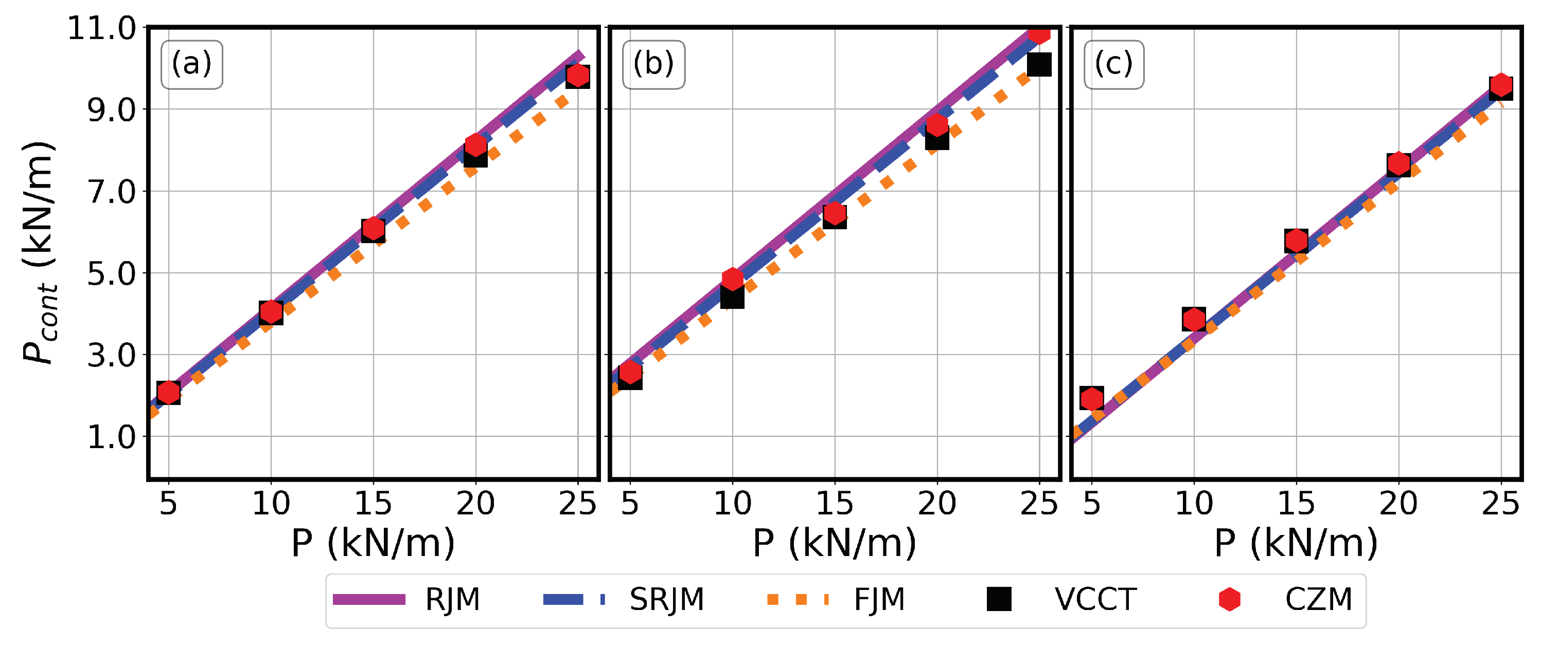
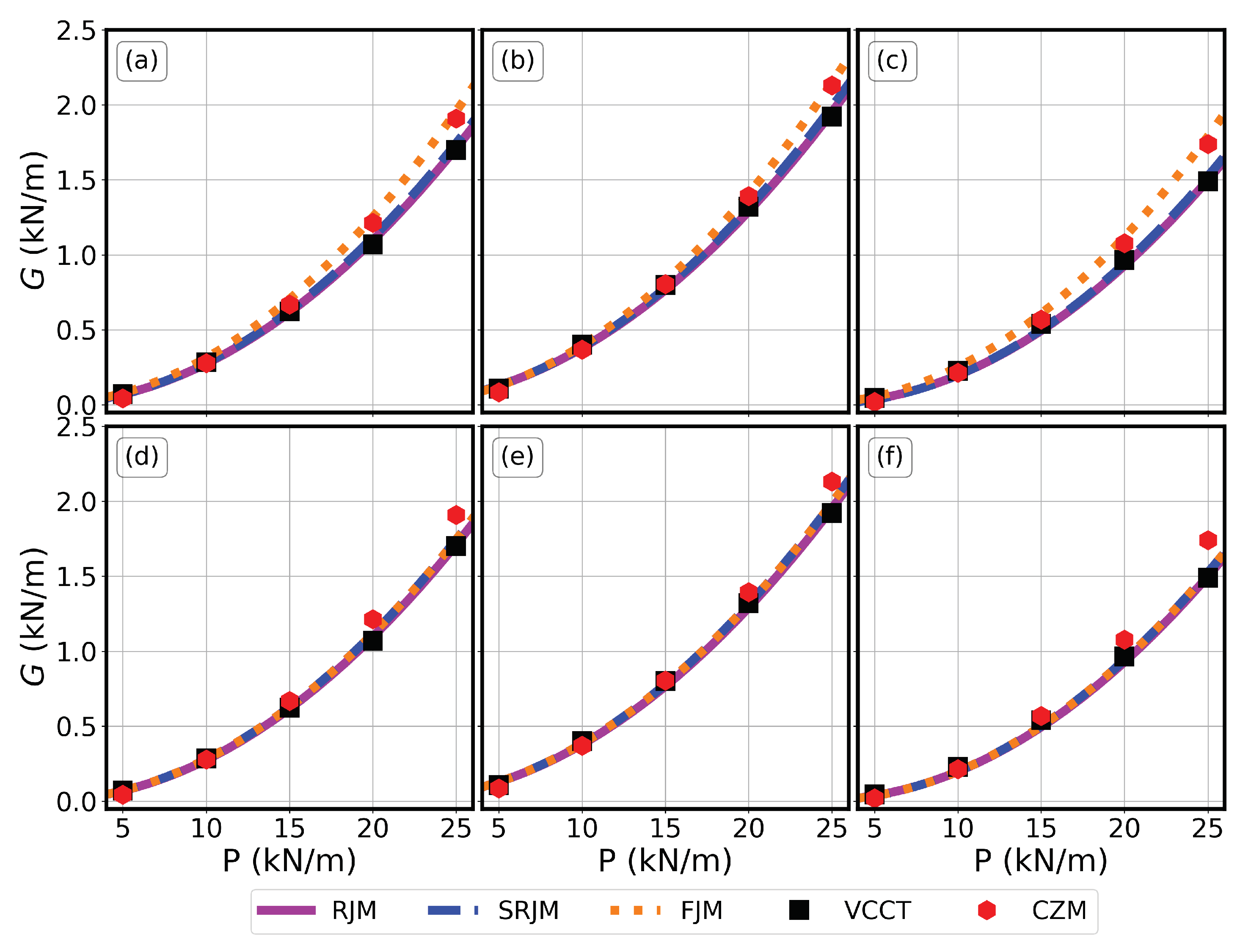
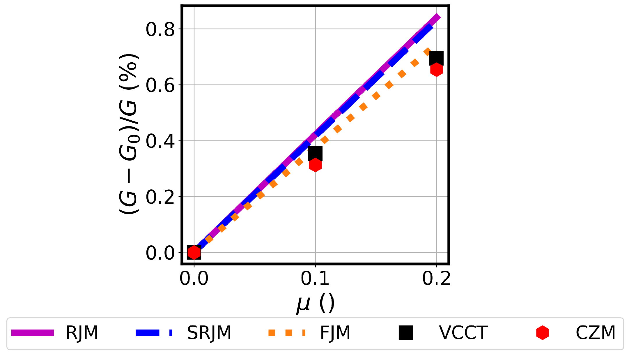
5.2. Energy Release Rate
6. Conclusions
Author Contributions
Funding
Institutional Review Board Statement
Informed Consent Statement
Data Availability Statement
Conflicts of Interest
Appendix A. Solutions of the Governing Equation
Appendix A.1. Rigid Joint Model
Appendix A.2. Semi-Rigid Joint Model
Appendix A.3. Flexible Joint Model
References
- Davies, P.; Blackman, B.; Brunner, A. Standard test methods for delamination resistance of composite materials: Current status. Appl. Compos. Mater. 1998, 5, 345–364. [Google Scholar] [CrossRef]
- Wang, J.; Qiao, P. Analysis of beam-type fracture specimens with crack-tip deformation. Int. J. Fract. 2005, 132, 223–248. [Google Scholar] [CrossRef]
- Polyzos, E.; Van Hemelrijck, D.; Pyl, L. Analytical model for the estimation of the hygrothermal residual stresses in generally layered laminates. Eng. Fract. Mech. 2021, 247, 107667. [Google Scholar] [CrossRef]
- Schapery, R.A.; Davidson, B.D. Prediction of energy release rate for mixed-mode delamination using classical plate theory. Appl. Mech. Rev. 1990, 43, S281–S287. [Google Scholar] [CrossRef]
- Yokozeki, T.; Ogasawara, T.; Aoki, T. Correction method for evaluation of interfacial fracture toughness of DCB, ENF and MMB specimens with residual thermal stresses. Compos. Sci. Technol. 2008, 68, 760–767. [Google Scholar] [CrossRef]
- Wang, J.; Qiao, P. Mechanics of bimaterial interface: Shear deformable split bilayer beam theory and fracture. J. Appl. Mech. 2005, 72, 674–682. [Google Scholar] [CrossRef]
- Sun, C.; Pandey, R. Improved method for calculating strain energy release rate based on beam theory. AIAA J. 1994, 32, 184–189. [Google Scholar] [CrossRef]
- Qiao, P.; Wang, J. Novel joint deformation models and their application to delamination fracture analysis. Compos. Sci. Technol. 2005, 65, 1826–1839. [Google Scholar] [CrossRef]
- Williams, J.G. End corrections for orthotropic DCB specimens. Compos. Sci. Technol. 1989, 35, 367–376. [Google Scholar] [CrossRef]
- Davidson, B.D.; Yu, L.; Hu, H. Determination of energy release rate and mode mix in three-dimensional layered structures using plate theory. Int. J. Fract. 2000, 105, 81–105. [Google Scholar] [CrossRef]
- Wang, J.; Qiao, P. On the energy release rate and mode mix of delaminated shear deformable composite plates. Int. J. Solids Struct. 2004, 41, 2757–2779. [Google Scholar] [CrossRef]
- Yokozeki, T. Energy release rates of bi-material interface crack including residual thermal stresses: Application of crack tip element method. Eng. Fract. Mech. 2010, 77, 84–93. [Google Scholar] [CrossRef]
- Yokozeki, T.; Block, T.B.; Herrmann, A.S. Effects of residual thermal stresses on the debond characterization of sandwich beams. J. Reinf. Plast. Compos. 2011, 30, 699–708. [Google Scholar] [CrossRef]
- Tsokanas, P.; Loutas, T. Hygrothermal effect on the strain energy release rates and mode mixity of asymmetric delaminations in generally layered beams. Eng. Fract. Mech. 2019, 214, 390–409. [Google Scholar] [CrossRef]
- Qiao, P.; Wang, J. Mechanics and fracture of crack tip deformable bi-material interface. Int. J. Solids Struct. 2004, 41, 7423–7444. [Google Scholar] [CrossRef]
- Kanninen, M. An augmented double cantilever beam model for studying crack propagation and arrest. Int. J. Fract. 1973, 9, 83–92. [Google Scholar] [CrossRef]
- Kanninen, M. A dynamic analysis of unstable crack propagation and arrest in the DCB test specimen. Int. J. Fract. 1974, 10, 415–430. [Google Scholar] [CrossRef]
- ASTM D5528-01; Standard Test Method for Mode I Interlaminar Fracture Toughness of Unidirectional Fiber-Reinforced Polymer Matrix Composites. American Standard of Testing Methods; ASTM International: West Conshohocken, PA, USA, 2014; Volume 3, pp. 1–12.
- ASTM D7905/D7905M-19e1; Standard Test Method for Determination of the Mode II Interlaminar Fracture Toughness of Unidirectional Fiber-Reinforced Polymer Matrix Composites. ASTM International: West Conshohocken, PA, USA, 2019.
- ISO 15114:2014; Fibre-Reinforced Plastic Composites—Determination of the Mode II Fracture Resistance for Unidirectionally Reinforced Materials Using the Calibrated End-Loaded Split (C-ELS) Test and an Effective Crack Length Approach. International Organization for Standardization: Geneva, Switzerland, 2014.
- Nairn, J.A. On the calculation of energy release rates for cracked laminates with residual stresses. Int. J. Fract. 2006, 139, 267–293. [Google Scholar] [CrossRef]
- Kageyama, K.; Kimpara, I.; Suzuki, T.; Ohsawa, I.; Kanai, M.; Tsuno, H. Effects of test conditions on mode II interlaminar fracture toughness of four-point ENF specimens. Energy 1999, 2, 362–370. [Google Scholar]
- Davidson, B.D.; Sun, X. Effects of friction, geometry, and fixture compliance on the perceived toughness from three-and four-point bend end-notched flexure tests. J. Reinf. Plast. Compos. 2005, 24, 1611–1628. [Google Scholar] [CrossRef]
- Sun, X.; Davidson, B.D. Numerical evaluation of the effects of friction and geometric nonlinearities on the energy release rate in three-and four-point bend end-notched flexure tests. Eng. Fract. Mech. 2006, 73, 1343–1361. [Google Scholar] [CrossRef]
- Bing, Q.; Sun, C. Effect of compressive transverse normal stress on mode II fracture toughness in polymeric composites. Int. J. Fract. 2007, 145, 89–97. [Google Scholar] [CrossRef]
- Parrinello, F.; Marannano, G.; Borino, G.; Pasta, A. Frictional effect in mode II delamination: Experimental test and numerical simulation. Eng. Fract. Mech. 2013, 110, 258–269. [Google Scholar] [CrossRef]
- Mencattelli, L.; Borotto, M.; Cugnoni, J.; Lazzeri, R.; Botsis, J. Analysis and evaluation of friction effects on mode II delamination testing. Compos. Struct. 2018, 190, 127–136. [Google Scholar] [CrossRef]
- Polyzos, E.; Van Hemelrijck, D.; Pyl, L. Extension-bending coupling phenomena and residual hygrothermal stresses effects on the Energy Release Rate and mode mixity of generally layered laminates. Int. J. Solids Struct. 2023, 277, 112297. [Google Scholar] [CrossRef]
- Reddy, J.N. Mechanics of Laminated Composite Plates and Shells: Theory and Analysis; CRC Press: Boca Raton, FL, USA, 2003. [Google Scholar]
- Zhang, C.; Wang, J. Delamination analysis of layered structures with residual stresses and transverse shear deformation. J. Eng. Mech. 2013, 139, 1627–1635. [Google Scholar] [CrossRef]
- Suhir, E. Stresses in bi-metal thermostats. J. Appl. Mech. 1986, 53, 647–660. [Google Scholar] [CrossRef]
- Wang, J.; Qiao, P. Novel beam analysis of end-notched flexure specimen for mode-II fracture. Eng. Fract. Mech. 2004, 71, 219–231. [Google Scholar] [CrossRef]
- Corleto, C.R.; Hogan, H.A. Energy release rates for the ENF specimen using a beam on an elastic foundation. J. Compos. Mater. 1995, 29, 1420–1436. [Google Scholar] [CrossRef]
- Williams, J.G. On the calculation of energy release rates for cracked laminates. Int. J. Fract. 1988, 36, 101–119. [Google Scholar] [CrossRef]
- Hashemi, S.; Kinloch, A.J.; Williams, J. The analysis of interlaminar fracture in uniaxial fibre-polymer composites. Proc. R. Soc. Lond. A Math. Phys. Sci. 1990, 427, 173–199. [Google Scholar]
- Polyzos, E. Stochastic analytical and numerical modelling of interface stressses for generally layered 3D-printed composites. In Proceedings of the 20th European Conference on Composite Mechanics: Composites Meet Sustainability, Lausanne, Switzerland, 26–30 June 2022; pp. 320–328. [Google Scholar]
- Polyzos, E.; Katalagarianakis, A.; Van Hemelrijck, D.; Pyl, L. Delamination analysis of 3D-printed nylon reinforced with continuous carbon fibers. Addit. Manuf. 2021, 46, 102144. [Google Scholar] [CrossRef]
- Bhat, S.; Narayanan, S. Quantification of fibre bridging in Mode I cracked Glare without delaminations. Eur. J. Mech. A/Solids 2014, 43, 152–170. [Google Scholar] [CrossRef]
- Smith, M. ABAQUS/Standard User’s Manual, Version 6.9; Dassault Systèmes Simulia Corp: Providence, RI, USA, 2009.
- Camanho, P.P.; Davila, C.G.; Ambur, D. Numerical simulation of delamination growth in layered composite plates. Eur. J. Mech. A/Solids 2001, 18, 291–312. [Google Scholar]
- Krueger, R. ICASE Report No 2002-10: The virtual crack closure technique: History, approach and applications. Appl. Mech. Rev. 2004, 57, 109–143. [Google Scholar] [CrossRef]
- Krueger, R. The Virtual Crack Closure Technique for Modeling Interlaminar Failure and Delamination in Advanced Composite Materials; Elsevier Ltd.: Amsterdam, The Netherlands, 2015; pp. 3–53. [Google Scholar]
- Dugdale, D. Yielding of steel sheets containing slits. J. Mech. Phys. Solids 1960, 8, 100–104. [Google Scholar] [CrossRef]
- Barenblatt, G.I. Mathematical Theory of Equilibrium Cracks in Brittle Failure. Adv. Appl. Mech. 1962, 7. [Google Scholar]
- Turon, A.; Dávila, C.; Camanho, P.; Costa, J. An engineering solution for mesh size effects in the simulation of delamination using cohesive zone models. Eng. Fract. Mech. 2007, 74, 1665–1682. [Google Scholar] [CrossRef]
- Rybicki, E.; Kanninen, M. A finite element calculation of stress intensity factors by a modified crack closure integral. Eng. Fract. Mech. 1977, 9, 931–938. [Google Scholar] [CrossRef]
- Benzeggagh, M.; Kenane, M. Measurement of mixed-mode delamination fracture toughness of unidirectional glass/epoxy composites with mixed-mode bending apparatus. Compos. Sci. Technol. 1996, 56, 439–449. [Google Scholar] [CrossRef]
- Polyzos, E.; Van Hemelrijck, D.; Pyl, L. An Open-Source ABAQUS Plug-In for Delamination Analysis of 3D Printed Composites. Polymers 2023, 15, 2171. [Google Scholar] [CrossRef] [PubMed]
- Suresha, B. The role of fillers on friction and slide wear characteristics in glass-epoxy composite systems. J. Miner. Mater. Charact. Eng. 2006, 5, 87. [Google Scholar] [CrossRef]
- Qiao, P.; Liu, Q. Energy release rate of beam-type fracture specimens with hygrothermal influence. Int. J. Damage Mech. 2016, 25, 1214–1234. [Google Scholar] [CrossRef]

| Aluminum | E-GFRP | Epoxy Resin | |
|---|---|---|---|
| (GPa) | 72.00 | 38.73 | 3.50 |
| (GPa) | 72.00 | 6.94 | 3.50 |
| (GPa) | 27.06 | 2.50 | 1.25 |
| 0.33 | 0.27 | 0.33 | |
| (10−6/°C) | 23.00 | 7.26 | 57.50 |
| (10−6/°C) | 23.00 | 37.70 | 57.50 |
Disclaimer/Publisher’s Note: The statements, opinions and data contained in all publications are solely those of the individual author(s) and contributor(s) and not of MDPI and/or the editor(s). MDPI and/or the editor(s) disclaim responsibility for any injury to people or property resulting from any ideas, methods, instructions or products referred to in the content. |
© 2024 by the authors. Licensee MDPI, Basel, Switzerland. This article is an open access article distributed under the terms and conditions of the Creative Commons Attribution (CC BY) license (https://creativecommons.org/licenses/by/4.0/).
Share and Cite
Polyzos, E.; Van Hemelrijck, D.; Pyl, L. Contact Force and Friction of Generally Layered Laminates with Residual Hygrothermal Stresses under Mode II In-Plane-Shear Delamination. Appl. Sci. 2024, 14, 7045. https://doi.org/10.3390/app14167045
Polyzos E, Van Hemelrijck D, Pyl L. Contact Force and Friction of Generally Layered Laminates with Residual Hygrothermal Stresses under Mode II In-Plane-Shear Delamination. Applied Sciences. 2024; 14(16):7045. https://doi.org/10.3390/app14167045
Chicago/Turabian StylePolyzos, Efstratios, Danny Van Hemelrijck, and Lincy Pyl. 2024. "Contact Force and Friction of Generally Layered Laminates with Residual Hygrothermal Stresses under Mode II In-Plane-Shear Delamination" Applied Sciences 14, no. 16: 7045. https://doi.org/10.3390/app14167045