A Closer Look at Few-Shot Classification with Many Novel Classes

Abstract

Few-shot learning (FSL) is designed to equip models with the capability to quickly adapt to new, unseen domains in open-world scenarios. However, there is a notable discrepancy between the multitude of new concepts encountered in the open world and the limited scale of existing FSL studies, which focus predominantly on a small number of novel classes. This limitation hinders the practical implementation of FSL in real-world situations. To address this issue, we introduce a novel problem called Few-Shot Learning with Many Novel Classes (FSL-MNC), which expands the number of novel classes more than 500 times compared to traditional FSL settings. This new challenge presents two main difficulties: increased computational load during meta-training and reduced classification accuracy due to the larger number of classes during meta-testing. To tackle these problems, we introduce the Simple Hierarchy Pipeline (SHA-Pipeline). In response to the inefficiency of traditional Episode Meta-Learning (EML) protocols, we redesign a more efficient meta-training strategy to manage the increased number of novel classes. Moreover, to distinguish distinct semantic features across a broad array of novel classes, we effectively reconstruct and utilize class hierarchy information during meta-testing. Our experiments demonstrate that the SHA-Pipeline substantially outperforms both the ProtoNet baseline and current leading alternatives across various numbers of novel classes.

1. Introduction

Few-shot learning (FSL) is a machine learning approach designed to enable models to quickly adapt to new tasks with very limited training data, often only a few examples per class. The “open-world scenario” refers to a dynamic and constantly changing environment where new, unseen classes can appear unexpectedly, and the learning model must be capable of recognizing and adapting to these novel classes efficiently [1].

The remarkable progress achieved by few-shot learning (FSL) [2] has endowed learning models with the capability to rapidly adapt to new visual concepts in an open world. Traditional FSL scenarios typically restrict the “scale” of this open world and the number of novel classes is often limited from 5 to 160 [3]. However, in a more realistic open-world setting, there can be a substantial amount of unseen knowledge, manifesting as thousands of novel classes, which far exceeds the range established by previous FSL protocols. Moreover, considering the number of novel classes is crucial for enhancing the practicality of FSL, given the impracticality of predicting the exact number of these classes in real-world applications (this paper is an extended version to our previous conference publication [4]).

Recent studies by Willes et al. [5] and Parmar et al. [6] emphasize that a genuine open-world learner for FSL should accommodate thousands of novel classes, such as those found in datasets like iNaturalist [6]. In response to these insights, we introduce a new problem setting named few-shot learning with many novel classes (FSL-MNC). Our approach significantly expands the conventional FSL framework by addressing scenarios with over 2000 novel classes, which represents more than a 10-fold increase compared to traditional settings. Here, few-shot tasks are structured as N-way K-shot episodes, where “way” and “shot” refer to the number of novel classes and the number of annotated samples per novel class, respectively. Unlike traditional settings where the ratio of novel to base class sizes is typically less than 1, in FSL-MNC, this ratio exceeds 10. To elucidate this expansion, we explore the few-shot generalization capabilities of models pre-trained on ImageNet-1k [7] meta-testing on non-overlapping classes from ImageNet-21K [8] as a motivating example.

In this example, we initially evaluate the efficiency and performance of established FSL algorithms such as ProtoNet and SimpleShot, illustrated in Figure 1. We observe that the computational overhead for meta-training escalates dramatically, from half an hour to over a hundred hours, as the number of ways increases. Concurrently, the performance of traditional FSL methods degrades substantially as the number of ways expands from the typical tens to the thousands, which is characteristic of our FSL-MNC paradigm. This underlines a significant research gap concerning the effectiveness of few-shot learning on a realistic scale.

In addressing the inefficiencies and sub-optimal performances of traditional FSL methods under the FSL-MNC setting, we identify challenges posed by the episodic meta-learning (EML) [9] framework. EML demonstrates a linear increase in computational demand with an increasing number of ways [10], particularly evident in large-scale scenarios. Moreover, in the context of FSL-MNC, the performance deterioration is notably severe when faced with a vast expansion in a number of ways. This deterioration is partly attributed to the challenges of classifying numerous fine-grained classes within a nested semantic hierarchy, as demonstrated in studies on ImageNet-21K and recent computer vision research [11,12,13]. Traditional FSL approaches often overlook such hierarchical structures due to the limited scale of novel classes they are designed to handle.

To address these challenges in FSL-MNC, we propose the novel Simple Hierarchy-Aware Pipeline (SHA-Pipeline). Our SHA-Pipeline introduces two primary strategies.

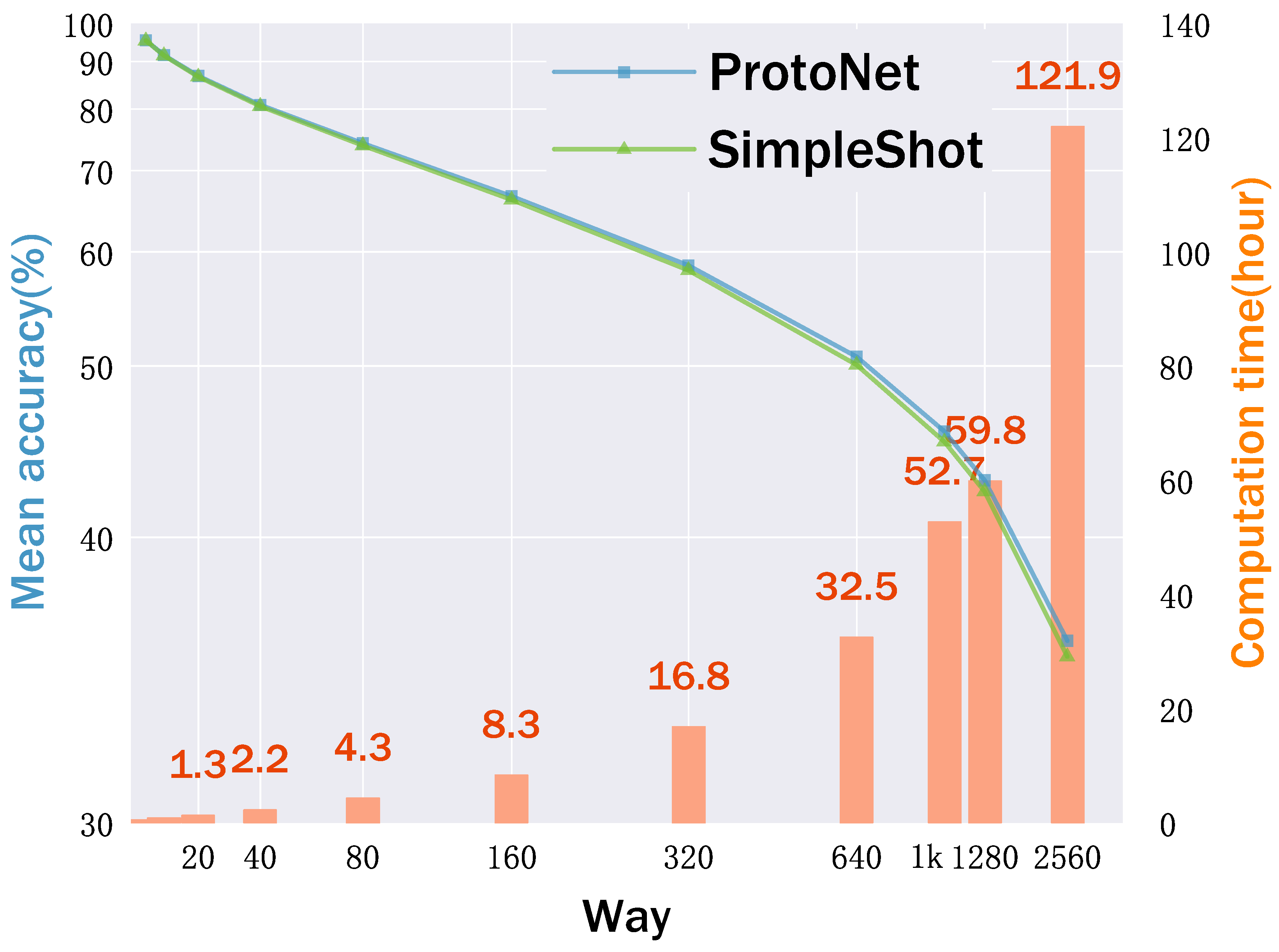
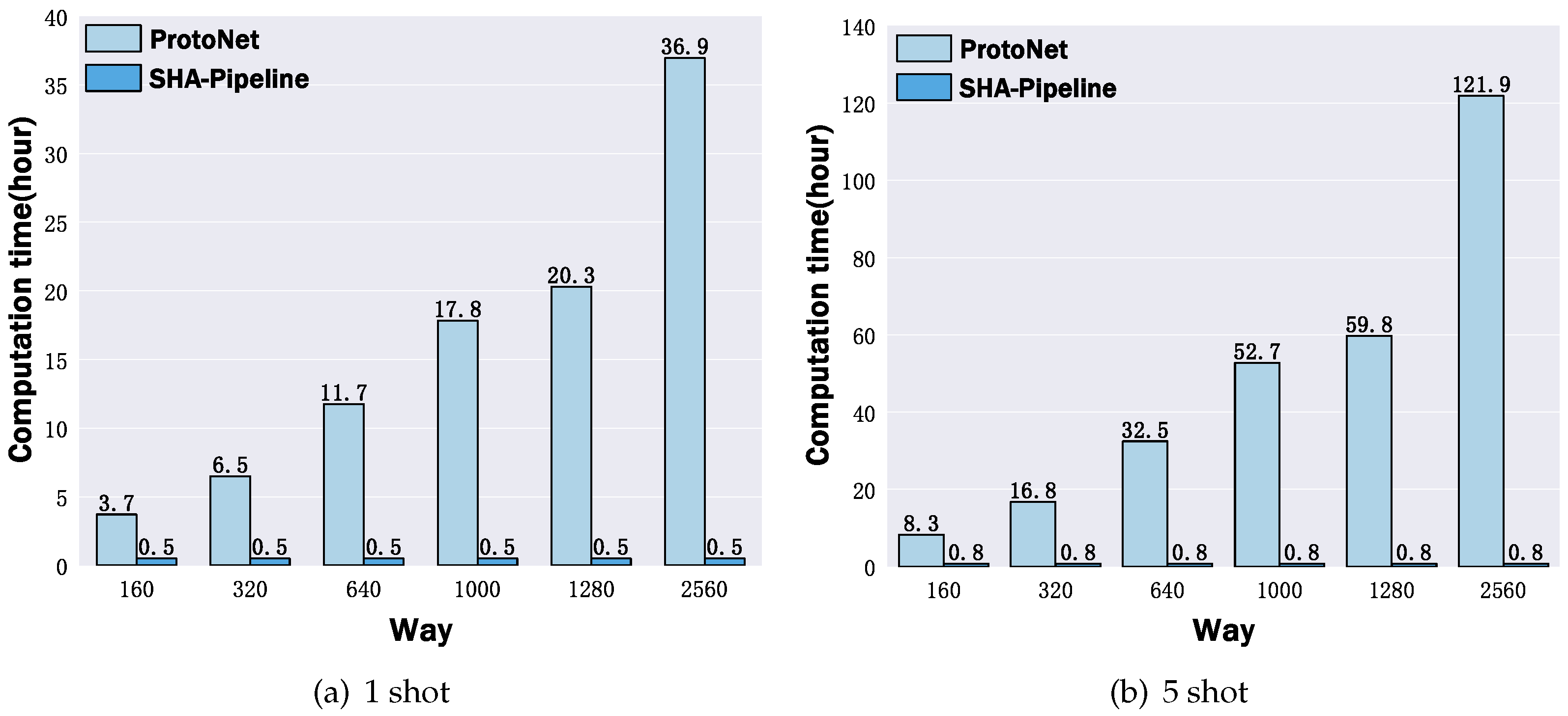
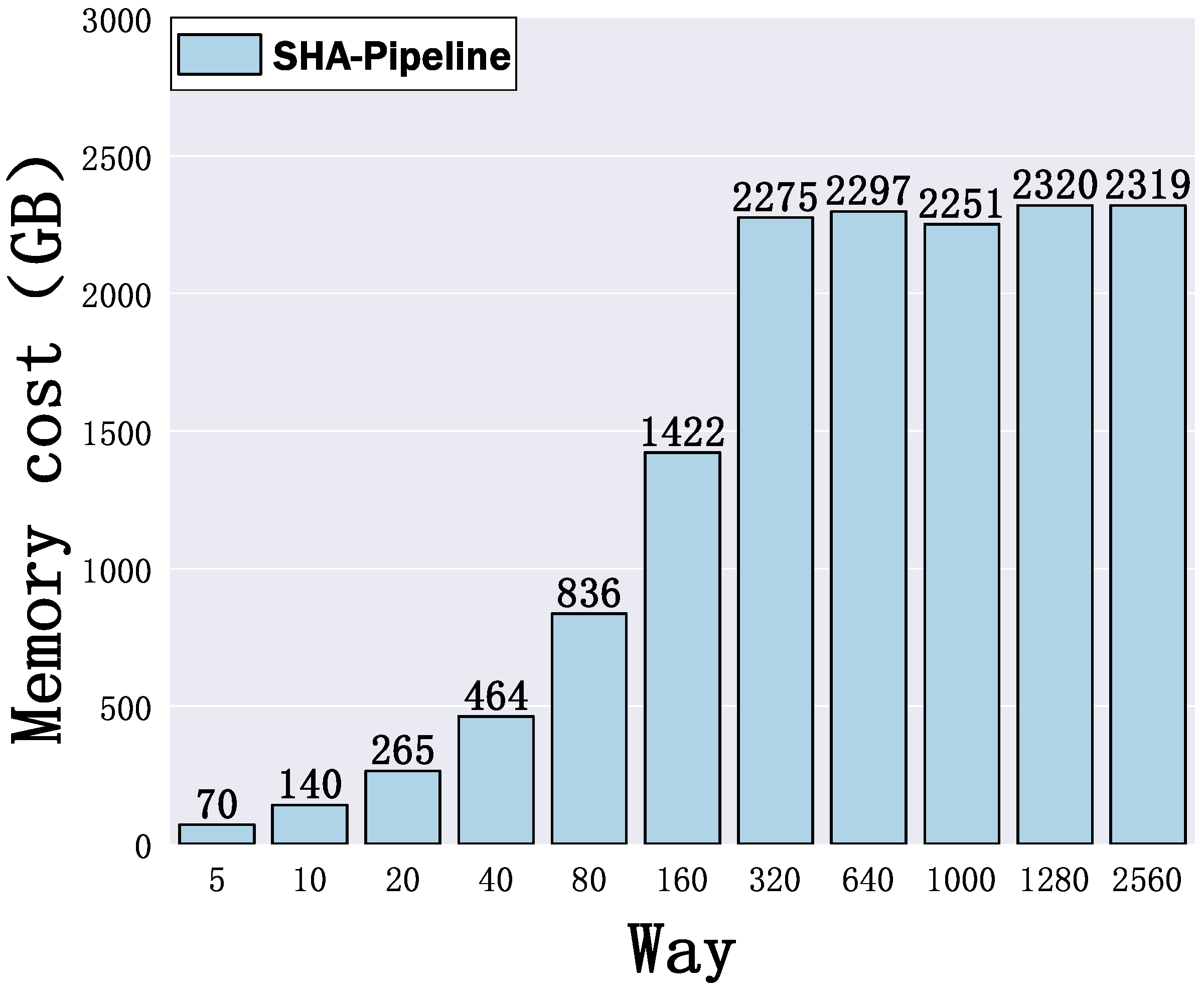
• Efficiency Enhancement. Our extensive experiments reveal that the efficiency of EML in FSL-MNC remains nearly constant across different numbers of ways when utilizing various backbones. By maintaining the number of ways in episodes at five, we significantly reduce the complexity associated with the number of ways in EML. Additionally, to expedite the training process, we minimize the communication overhead of support samples and avoid GPU memory overflow by efficiently distributing the support and partial query sets, as shown in Section 5.3.
• Performance Improvement. We enhance classification performance by employing a fast, non-parametric hierarchy clustering strategy to capture the class hierarchy, and then we leverage such class hierarchy by structured representation learning. This approach enhances representation learning on two levels: prototype-level and sample-level. At the prototype level, we strive to maintain the hierarchical structure of class prototypes by maximizing the Cophenetic Correlation Coefficient (CPCC). At the sample level, we use hierarchical triplet loss to ensure that similar samples from different parent classes remain distinctly separate.

The contributions of our paper are as follows. We propose the “few-shot learning with many novel classes (FSL-MNC)” setting to bridge the gap between traditional few-shot learning and realistic open-world scenarios, presenting a practical yet underexplored challenge. Our SHA-Pipeline efficiently addresses both computational and performance challenges by reducing meta-training overhead to a constant level and utilizing class hierarchy during meta-testing. Experimental results demonstrate that the SHA-Pipeline efficiently outperforms state-of-the-art alternatives across various novel class sizes.

The extension of our journal paper from our previous conference publication [4] is outlined as follows. In this journal article, we provide a more detailed description and analysis of our proposed problem setting and method in Section 3 and Section 4, respectively, to ensure the completeness of the model. To strengthen our experimental results, we extend our experiments and include a more detailed analysis of the meta-training strategy and computation overhead in Section 5.2 and Section 5.3, respectively. Additionally, we evaluate our methodology on traditional FSL benchmarks in Section 5.5 and conduct visualization experiments in Section 5.7.

The remainder of our work is organized as follows: We present related work in Section 2. Section 3 formulates our problem setting. Section 4 describes our models in detail. Section 5 provides experimental analysis, followed by the conclusion and future work in Section 6.

2. Related Work

2.1. Traditional Few-Shot Learning

Few-shot learning (FSL) is a rapidly evolving research area, with significant contributions that enhance the ability to quickly adapt to new, unseen tasks. Comprehensive reviews by Hospedales et al. [14] and Wang et al. [2] provide an in-depth look at the field. Various methods have been proposed to tackle FSL challenges, including meta-learning approaches like those introduced by Vinyals et al. [15] and Ravi and Larochelle [16], as well as metric-based methods such as those developed in Ye et al. [17] and Ye and Chao [18], all of which demonstrate robust performance on FSL benchmarks.

However, the majority of existing FSL methodologies are geared toward tasks involving a relatively small number of novel classes. This limitation significantly hinders their applicability in realistic, large-scale open-world settings [6,19]. For instance, gradient-based frameworks like MAML [20] struggle with scalability across varying numbers of ways. Furthermore, state-of-the-art few-shot metric-based methods, such as FEAT [17], incur considerable computational overheads during meta-training when scaled up. Simpler baselines, such as SimpleShot [21], fail to efficiently utilize structural information inherent in larger tasks.

2.2. Large-Scale Few-Shot Learning

While a few studies [3,22,23,24] have ventured into applying FSL on larger datasets, they have not fully explored the challenges associated with an increased number of novel classes in the meta-testing phase, which represents a more practical and challenging scenario. Notably, Liu et al. [23] and Li et al. [24] utilize external class hierarchy structures rather than deriving them from the few-shot data itself. Hu et al. [22] continue to rely on traditional episodic training methods, which do not scale well with an increasing number of ways. Dhillon et al. [3], meanwhile, do not address the scalability issues in the meta-training stage when dealing with a large number of ways. Our work diverges from these approaches by specifically investigating the efficacy of simple baselines under scenarios where the number of ways is significantly expanded. For instance, the size of novel classes dataset in previous researches [3,22,23,24] is less than 1000, while the number of unseen classes in open-world scenarios is typical larger than 1000.

2.3. FSL with Class Hierarchy

The exploration of class hierarchy in few-shot learning has been limited, with notable exceptions being the works of Li et al. [24] and Liu et al. [23]. These studies incorporate class hierarchy information, though typically sourced from pre-existing databases or learned from public text corpora, deviating from the foundational few-shot learning premise. In contrast, our Simple Hierarchy-Aware Pipeline (SHA-Pipeline) uniquely captures class hierarchy directly from the few-shot tasks themselves through recursive nonparametric clustering [25].

For the mining of class hierarchy structures in the meta-testing phase, we employ a non-parametric hierarchical clustering method that features low computational overhead, as recently proposed. Differently from previous approaches, we apply Z-score normalization [26] to instance embeddings to mitigate the hubness problem before performing hierarchical clustering on class prototypes. This method ensures a more effective and scalable approach to understanding and leveraging class hierarchies in FSL contexts.

3. Few-Shot Learning with Many Novel Classes

3.1. Problem Formulation

We first introduce the formulation of few-shot learning and then define few-shot learning with many novel classes. After that, we offer the definition of class hierarchical structure in the context of few-shot learning.

3.1.1. Few-Shot Learning

We let $C_{\mathrm{base}}$ and $C_{\mathrm{novel}}$ denote the set of base and novel classes, respectively, which are disjoint, i.e., $C_{\mathrm{base}}\cap C_{\mathrm{novel}}=\varnothing$. Given the datasets $D_{\mathrm{base}}$ and $D_{\mathrm{novel}}$ containing labeled samples from $C_{\mathrm{base}}$ and $C_{\mathrm{novel}}$, respectively, the objective of FSL is to train model $f_{\varphi }$ using $D_{\mathrm{base}}$ to perform effectively on few-shot tasks sampled from $D_{\mathrm{novel}}$. Each task ${\mathcal{T}}_i$ comprises a support set ${\mathcal{S}}^i={\left\{\left({\mathbf{x}}_j,{\mathbf{y}}_j\right)\right\}}_{j=1}^{N\times k}$ and a query set ${\mathcal{Q}}^i={\left\{\left({\tilde{\mathbf{x}}}_j,{\tilde{\mathbf{y}}}_j\right)\right\}}_{j=1}^{N\times q}$, where ${\mathcal{S}}^i$ contains N classes with k labeled examples per class, and ${\mathcal{Q}}^i$ features q unlabeled query examples per class. The terms N and k are commonly referred to as “way” and “shot”, respectively.

3.1.2. Few-Shot Learning with Many Novel Classes

A higher value of N indicates a greater degree of “novelness” associated with a few-shot episode. This implies that as N increases, the few-shot tasks necessitate a broader level of adaptation to incorporate the new knowledge presented in the open-world scenario.

In the realm of FSL-MNC, the value of N often far exceeds that found in conventional few-shot learning contexts (e.g., $N>1000$), posing significant computational and generalization challenges. We introduce a metric designed to quantify the level of “novelness” inherent within a given few-shot dataset. This metric helps distinctly classify FSL-MNC from traditional FSL approaches, highlighting their inherent differences. The novelness ratio, denoted as $\Omega \left(D_{\mathrm{novel}};D_{\mathrm{base}}\right)$, is defined as the ratio of the size of the novel class set to that of the base class set:

$$\Omega \left(D_{\mathrm{novel}};D_{\mathrm{base}}\right)={\displaystyle \frac{|C_{\mathrm{novel}}|}{|C_{\mathrm{base}}|}}$$

(1)

Figure 2 illustrates a comparison of the novel class set sizes and the novelness ratio exhibited by both traditional few-shot datasets and our ImageNet-MNC dataset (15,000 novel classes and 1000 base classes) tailored for the FSL-MNC benchmark. In traditional FSL, the novelness ratio $\Omega \left(D_{\mathrm{novel}};D_{\mathrm{base}}\right)$ is typically less than one (the red bar in Figure 2), indicating a relatively small number of novel classes compared to base classes. Conversely, in FSL-MNC, $\Omega \left(D_{\mathrm{novel}};D_{\mathrm{base}}\right)>10$, signifying a substantial increase in the number of novel classes relative to the base classes.

Mathematically, the FSL-MNC challenge can be precisely described as follows: Given the datasets $D_{\mathrm{base}}$ and $D_{\mathrm{novel}}$ where the condition $\Omega \left(D_{\mathrm{novel}};D_{\mathrm{base}}\right)>10$ is met, the primary goal is to train model $f_{\varphi }$ using $D_{\mathrm{base}}$, which can effectively handle few-shot tasks derived from $D_{\mathrm{novel}}$ with a way number $N > |C_{\mathrm{base}}|$.

3.1.3. Class Hierarchical Structure

In addressing FSL-MNC, we utilize a class hierarchy to enhance model performance. The formal definition of this class hierarchy is represented by a Directed Acyclic Graph (DAG), denoted as $\mathcal{G}=(\mathcal{V},\mathcal{E})$, where $\mathcal{V}=\mathcal{C}\cup \mathcal{R}$. Here, $\mathcal{C}$ comprises specific classes, and $\mathcal{R}$ consists of abstract parent classes. This graph forms a single tree, with leaf nodes corresponding to specific classes from $\mathcal{C}$ and non-leaf nodes from $\mathcal{R}$ representing abstract parent classes encompassing subsets of specific classes. Relationships between nodes are defined by $\mathcal{E}\subseteq \left\{(x,y)\mid (x,y)\in {\mathcal{V}}^2\right\}$, indicating parent–child connections.

The tree’s height, denoted as H, reflects the length of the path from the root node to its leaf nodes. For any specific class $c_i\in \mathcal{C}$, a set of parent classes ${\mathcal{A}}^{c_i}=\left\{{\mathcal{P}}_1^{c_i},{\mathcal{P}}_2^{c_i},\cdots ,{\mathcal{P}}_H^{c_i}\right\}$ is derived by tracing the shortest path from $c_i$ to the root node. Each ${\mathcal{P}}_h^{c_i}$ represents an ancestor node of $c_i$ at the hth level of $\mathcal{G}$.

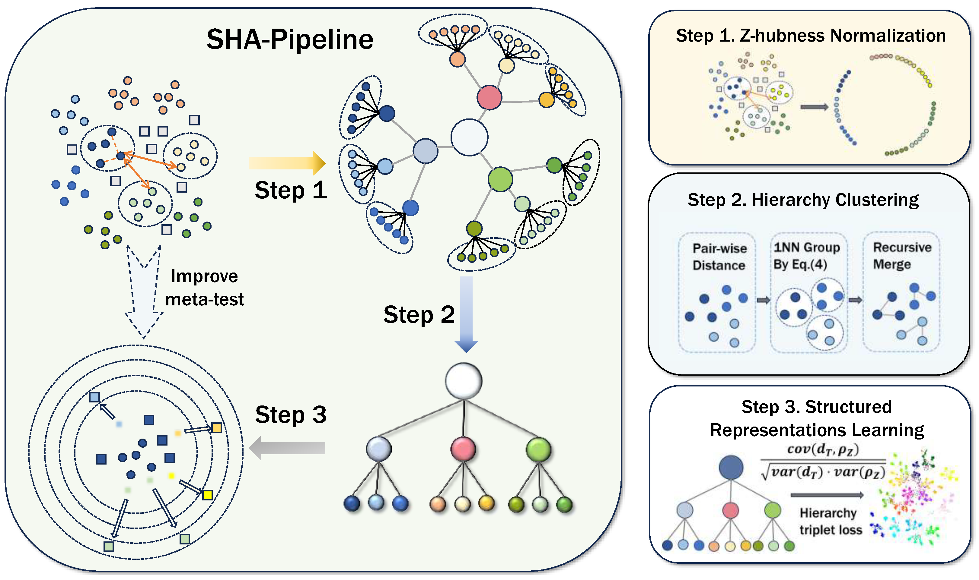
4. Simple Hierarchy-Aware Pipeline

To address the computational challenges posed by FSL-MNC, we introduce a meta-training strategy marked by efficiency and supported by comprehensive experimentation. Additionally, we design a lightweight distributed framework tailored for performance optimization in FSL-MNC scenarios. We propose a fine-tuning algorithm that effectively harnesses the potential of class hierarchy, facilitating improved integration and utilization of class-specific features.

4.1. Enhancing Efficiency

In traditional FSL, a learning function $f(·)$ is trained using a sequence of N-way K-shot tasks sampled from a base dataset. The objective of this training is to optimize $f(·)$ to minimize the average error across these tasks, as shown in the following equation:

$$f^{*}=\underset{f}{argmin}\sum _{\left({\mathcal{S}}^i,{\mathcal{Q}}^i\right)\in {\mathcal{T}}^i}\sum _{\left(\mathbf{x},\mathbf{y}\right)\in {\mathcal{Q}}^i}\mathsf{\ell }\left(f\left(\mathbf{x};{\mathcal{S}}^i\right),\mathbf{y}\right),$$

(2)

where $\mathsf{\ell }(·)$ denotes the loss function and ${\mathcal{S}}^i$ and ${\mathcal{Q}}^i$ represent the support and query sets from ${\mathcal{T}}^i$, respectively. In traditional setups, the N in meta-training and meta-testing usually matches in magnitude.

4.1.1. A Strategy for Meta-Learning

In the context of FSL-MNC, we observed that the performance during meta-training not only surpasses the SimpleShot approach but also shows that this improvement is relatively independent of the way number, as evidenced by extensive experiments across different backbones. The detailed results are depicted in Section 5.2. Considering the effectiveness of simple meta-training strategies on five-way episodes in enhancing performance on FSL-MNC tasks, we continue to utilize an $N=5$ configuration during our meta-training phase in the SHA-Pipeline.

We also compare pre-training and meta-training. The prevailing view in traditional FSL suggests that meta-learning may not always outperform a well-trained embedding model. Simple, non-episodic training methods based on a pre-trained backbone can yield performance comparable to more complex meta-training approaches. Common baseline methods build upon transfer learning strategies, adapting to few-shot target data through various feature-transformation methods. However, FSL-MNC stands apart due to its wider range of tasks during the meta-training phase, enhancing the generalization capabilities of meta-learning, a perspective supported by recent research. This divergence in approach highlights the unique benefits of meta-learning in settings with high task diversity.

4.1.2. Lightweight Parallel Framework

For further acceleration of EML training, we propose a parallel framework that distributes the entire support set and segments of the query set across multiple GPUs. This approach minimizes the need for inter-GPU communication of support sets and prevents GPU memory overflow. The comprehensive details of this framework are provided in Algorithm 1.

In the meta-testing phase of this experiment, the fine-tuning algorithm based on CPCC utilized global gradients. To avoid memory overflow during meta-testing, the experiment adopted a method of using small-batch gradient updates to estimate the single-step global gradient updates. For each instance of single-step global gradient fine-tuning, the query set on each GPU was further divided into multiple blocks. This allowed for the performance of backpropagation and synchronized updates on these smaller blocks, effectively replacing the global gradient and thereby substantially reducing memory requirements during training. An overview of the meta-testing parallel framework is provided in Algorithm 2. The symbol ∼ in our algorithms denotes sampling from a distribution.

Algorithm 1: A Lightweight Parallel Framework for meta-training

Require: $p\left(\mathcal{T}\right)$: distribution over tasks Require: $\alpha$: step size hyperparameters, n: GPU numbers 1: load pre-trained weights $\theta$ 2: while not done do 3:    Sample a few-shot task ${\mathcal{T}}_i=\left({\mathcal{S}}^i,{\mathcal{Q}}^i\right)\sim p\left(\mathcal{T}\right)$ 4:    Split ${\mathcal{Q}}^i$ into $\{{\mathcal{Q}}_0^i,{\mathcal{Q}}_1^i,\dots ,{\mathcal{Q}}_n^i\}$ 5:    Send $\left({\mathcal{S}}^i,{\mathcal{Q}}_j^i\right)$ to GPU j. 6:    for all GPU i do 7:       Evaluate ${\nabla }_{\theta }{\mathcal{L}}_{{\mathcal{T}}_i}\left(f_{\theta }\right)$ with respect to $\left({\mathcal{S}}^i,{\mathcal{Q}}_j^i\right)$ 8:    end for 9:    Allreduce ${\nabla }_{\theta }{\mathcal{L}}_{{\mathcal{T}}_i}\left(f_{\theta }\right)$ among GPUs 10:   Update adapted parameters with gradient descent: $\theta =\theta -\alpha {\nabla }_{\theta }{\mathcal{L}}_{{\mathcal{T}}_i}\left(f_{\theta }\right)$ 11: end while

Algorithm 2: A Lightweight Parallel Framework for meta-testing

Require: $p\left(\mathcal{T}\right)$: distribution over tasks Require: $\alpha$: step size hyperparameters, n: GPU numbers 1: Load pre-trained weights $\theta$ 2: Sample a few-shot task ${\mathcal{T}}_i=\left({\mathcal{S}}^i,{\mathcal{Q}}^i\right)\sim p\left(\mathcal{T}\right)$ 3: Split ${\mathcal{Q}}^i$ into ${\mathcal{Q}}_0^i,{\mathcal{Q}}_1^i,\dots ,{\mathcal{Q}}_n^i$ 4: Send $\left({\mathcal{S}}^i,{\mathcal{Q}}_j^i\right)$ to GPU j 5: while not done do 6:    for all GPU g do 7:       random sample ${\mathcal{Q}}_{random}^i$ from ${\mathcal{Q}}_g^i$ 8:       Evaluate ${\nabla }_{\theta }{\mathcal{L}}_{{\mathcal{T}}_i}\left(f_{\theta }\right)$ based on $\left({\mathcal{S}}^i,{\mathcal{Q}}_{random}^i\right)$ 9:    end for 10:   Allreduce ${\nabla }_{\theta }{\mathcal{L}}_{{\mathcal{T}}_i}\left(f_{\theta }\right)$ between all GPUs 11:   Update adapted parameters with gradient descent: $\theta =\theta -\alpha {\nabla }_{\theta }{\mathcal{L}}_{{\mathcal{T}}_i}\left(f_{\theta }\right)$ 12: end while

4.2. Fine-Tuning with Class Hierarchy Capturing

Next, we focus on the meta-testing stage of the SHA-Pipeline, illustrated in Figure 3. This stage involves a three-step fine-tuning process for each few-shot task. Initially, class prototypes are computed with Z-hubness normalization applied to feature vectors. This is followed by parameter-free hierarchical clustering of these prototypes. Based on the results of this clustering, a tree-metric distance matrix $\mathcal{T}={\left\{t(c_i,c_j)\right\}}_{c_i,c_j\in \mathcal{C}}$ of prototype pairs is calculated. Utilizing $\mathcal{T}$ as supervisory data, we fine-tune the backbone guided by cross-entropy loss supplemented with CPCC regularization or hierarchy triplet loss. The fine-tuning algorithm, based on CPCC normalization, is detailed in Algorithm 3, with a variant based on hierarchy triplet loss easily derivable from it.

Algorithm 3: Algorithm for Fine-Tuning

Require: N-way M-shot episodes (${\mathcal{D}}_{\mathbf{train}}^{\mathcal{S}}$, ${\mathcal{D}}_{\mathbf{test}}^{\mathcal{S}}$), learning rate $\eta$, fine-tune step I, backbone weights $\varphi$ 1: Load model from $\varphi$ 2: for all iteration = 1, …, I do 3:    ${\mathcal{D}}_{\mathbf{aug}}^{\mathcal{S}}=\mathrm{data\_augment}\left({\mathcal{D}}_{\mathbf{train}}^{\mathcal{S}}\right)$ 4:    Feature forward and normalization via Equation (3) 5:    Compute prototypes and cosine distance 6:    Hierarchy clustering 7:    Compute tree distance via Equation (5) 8:    Compute ${\mathcal{L}}_{train}$ via Equation (7) 9:    Update $\varphi$ with ${\mathcal{L}}_{train}$ using SGD 10: end for 11: Compute logits ${\sigma }_{\mathbf{test}}$ with updated $\varphi$  12: return ${\sigma }_{\mathbf{test}}$.

4.2.1. Z-Hubness Normalization

To address the hubness problem inherent in high-dimensional spaces before hierarchical clustering, we employ Z-hubness normalization on the feature vectors. This normalization adjusts the feature vectors to a consistent scale and distribution, thus facilitating more effective clustering and minimizing the influence of outlier features. The Z-score normalized feature is given by

$${\mathbf{x}}^{\left(zn\right)}={\displaystyle \frac{\mathbf{x}-\mu \mathbf{1}}{\sigma }}\in {\mathbb{R}}^D,$$

(3)

where $\mu$ and $\sigma$ are the mean and standard deviation of components of the feature vector $\mathbf{x}$, respectively.

4.2.2. Hierarchical Clustering with the First Neighbor

Utilizing a rapid hierarchical clustering algorithm, we process the adjacency link matrix of class prototypes. The adjacency link matrix can be represented as

$$A(i,j)=\left\{\begin{array}{cc}1\hfill & \mathrm{if}j={\kappa }_i^1\mathrm{or}{\kappa }_j^1=i\mathrm{or}{\kappa }_i^1={\kappa }_j^1\hfill \\ 0\hfill & \mathrm{otherwise}\hfill \end{array}\right.,$$

(4)

where $\mathbf{A}$ is the adjacency matrix, i and j represent sample indices, ${\kappa }_i^1$ symbolizes the first neighbor of point i.

This matrix determines clustering based on the nearest neighbor relationships, thereby forming clusters that reflect the natural groupings within the data. This method of clustering provides a robust basis for further fine-tuning and optimization of the learning model.

4.2.3. Structured Representation Learning with Class Hierarchy

To fully leverage the class hierarchy, we explore two approaches to structure the learning process. One approach employs a metric-level constraint to ensure that Euclidean distances between prototypes closely approximate the theoretical distances defined by the class hierarchy. Another approach uses hierarchy triplet loss, which imposes sample-level constraints to maintain distance between similar samples from the same parent classes.

CPCC Regularization. Firstly, we define the distance between prototype i and prototype j on the class hierarchy $d_T(i,j)$ as follows:

$$d_T(i,j)=H-\sum _{k=1}^H\left(\mathbb{I}\left(r_i^{\left(k\right)}=r_j^{\left(k\right)}\right)\right),$$

(5)

where $r_i$ represents the hierarchy cluster result of the prototype i, with kth element $r_i^{\left(k\right)}$ indicating the cluster ID to which the prototype belongs at level k. H represents the overall height of the class hierarchy, which is greater than one. $\mathbb{I}$ is the indicator function, and the range of $d_T(i,j)$ spans the interval $[1,H]$.

To quantify the alignment between the class hierarchy and feature transformations, we incorporate Cophenetic Correlation Coefficient (CPCC) regularization. The CPCC measures the correlation between the class hierarchy distances and the cosine distances between class prototypes, computed as follows:

$$CPCC\left(d_T,{\rho }_{\mathcal{Z}}\right)={\displaystyle \frac{cov\left(d_T,{\rho }_Z\right)}{\sqrt{var\left(d_T\right)·var\left({\rho }_Z\right)}}}$$

(6)

where $d_T$ and ${\rho }_Z$ represent the sets of pairwise class hierarchy and cosine distances, respectively. $cov(·)$ and $var(·)$ denote the covariance and variance, respectively.

The total training loss is a combination of cross-entropy loss $\left({\mathcal{L}}_{\mathrm{CE}}\right)$ and the CPCC regularization term $\left(\mathrm{CPCC}\right)$, leading to the following formulation:

$${\mathcal{L}}_{train}=\sum _{(x,y)\in \tilde{\mathcal{S}}}{\mathsf{\ell }}_{\mathrm{CE}}\left(y,g\left(f_{\theta }\left(x\right)\right)\right)-\lambda ·CPCC\left(d_T,{\rho }_Z\right),$$

(7)

where $\lambda$ is the weighting factor for the CPCC regularization term and $\tilde{\mathcal{S}}$ represents the data-augmented support set for the few-shot task.

Hierarchy triplet loss. In the following, we also offer another way to learn structured representation with class hierarchy based on triplet loss with adaptive margin.

We re-scale the $d_T(i,j)$ to the interval $[0,1)$ to obtain the adaptive margin $M(i,j)$ between anchor prototype i and negative prototype j:

$$M(i,j)={\displaystyle \frac{d_T(i,j)\left(1-d_{mean}\right)}{H}}+d_{mean}-d_i+d_j,$$

(8)

where $d_i$ and $d_j$ are the average cosine distance of the samples from class i and class j, respectively. $d_{mean}$ is given by $d_{mean}={\displaystyle \frac{1}{\mathcal{C}}}{\sum }_{i=1}^N{d}_i$.

After obtaining the adaptive margin $M(i,j)$, for the sake of computation overhead, we randomly sample triplets ${\mathcal{T}}_z=\left({\mathit{x}}_a,{\mathit{x}}_p,{\mathit{x}}_n\right)$ from the data-augmented support set $\tilde{\mathcal{S}}$ and obtain the corresponding adaptive margin $M(i,j)$ for sample $x_a$ and negative sample $x_n$ which comes from the ith class and the jth class, respectively. The hierarchy triplet loss is given by

$${\mathcal{L}}_{htl}={\displaystyle \frac{1}{|{\mathcal{T}}^{\mathcal{M}}|}}\sum _{{\mathcal{T}}^z\in {\mathcal{T}}^{\mathcal{M}}}{\left[{∥{\mathit{x}}_a-{\mathit{x}}_p∥}^2-{∥{\mathit{x}}_a-{\mathit{x}}_n∥}^2+M(i,j)\right]}_{+}$$

(9)

5. Experiments

In this section, the performance of various advanced methods suitable for FSL-MNC is compared. The results indicate that SHA-Pipeline not only effectively reduces the computational overhead in FSL-MNC but also addresses the challenges of class scalability brought about by the increase in new classes through fine-tuning based on class hierarchy, thereby enhancing classification accuracy. Experiments were not only conducted in FSL-MNC, but were also validated in standard few-shot learning settings, demonstrating the broad applicability of SHA-Pipeline. Additionally, this section includes an ablation study.

5.1. Experimental Setup

5.1.1. Datasets

This paper introduces ImageNet-MNC, a novel dataset tailored for FSL-MNC. The base class set is derived from ImageNet-1k (ILSVRC 2012–2017) [7], a benchmark widely utilized in image classification comprising 1000 categories. Furthermore, the recently released ImageNet-21K (winter ’21 version) [7] provides the novel class set, featuring a vast and diverse collection of over 21,000 categories.

To assemble ImageNet-21K-MNC, the study initially removed all 1000 categories that overlapped with ImageNet-1k from ImageNet-21K, preserving the uniqueness of the new dataset. Subsequently, categories containing fewer than 20 samples were excluded, amounting to 1455, to ensure each category had adequate data for effective training and testing.

After refining the dataset, a total of 16,712 viable categories remained. For the meta-learning experiments, 15,000 of these categories were randomly chosen for meta-testing to evaluate the model’s generalization capabilities on unseen classes. The remaining 1712 categories served as a validation set in the meta-training phase, facilitating the tuning and optimization of model parameters.

The dataset’s partition strategy ensures a strict separation between training and testing categories and enables performance assessment of various models within a cohesive and intricate framework. The design of ImageNet-MNC caters to the demands of large-scale, challenging classification tasks prevalent in modern machine learning, particularly deep learning, and aims to propel advancements in few-shot learning, transfer learning, and related fields.

In addition to the proprietary dataset, the experiments also employed several publicly available few-shot learning datasets, including miniImageNet [15], CIFAR-FS [27], and Meta-Dataset [28]. These datasets were strictly non-overlapping in training and testing phases, adhering to the setup where base and novel classes do not overlap.

miniImageNet, a subset of ImageNet-1k, contains 100 categories, each with 600 samples. Following established protocols [17], 64 categories were utilized as seen classes, with the remaining 16 and 20 categories serving as unseen classes for model validation and evaluation, respectively. CIFAR-FS is organized into 64 training categories, 16 validation categories, and 20 testing categories, with images sized at 32 × 32.

Additionally, this study explored the cross-domain few-shot generalization capabilities of SHA-Pipeline using the Meta-Dataset, which encompasses 10 public image datasets across various domains: ImageNet-1k, Omniglot, FGVC Aircraft, CUB-200-2011, Describable Textures, QuickDraw, FGVCx Fungi, VGG Flower, Traffic Signs, and MSCOCO. Each dataset includes distinct training, validation, and testing splits. To prevent novel class leakage during pre-training, the experimental protocol set by previous research [29] was adhered to considering only the training split of ImageNet-1k for meta-training, with testing sets from all datasets used for meta-testing. For additional details on the Meta-Dataset, refer to Appendix 3 of the related study [28].

5.1.2. Experimental Protocols

To ensure fairness in experimental setups and to avoid over-engineered designs, this paper selects publicly available backbone networks pretrained on the ImageNet-1k dataset. For the backbone network selection, this paper utilizes ViT [30] and ResNet50 [31]. Additionally, the paper employs various pretraining strategies, including supervised pretraining [31] (abbreviated as Sup), DINO [32], Deit [33], and MAE [34].

DINO, a self-supervised learning algorithm proposed by the Facebook AI Research team, trains Transformer models to learn meaningful features from unlabeled data through a label-free self-distillation process. Deit, also by Facebook AI Research, is a method for efficiently training vision Transformers by combining knowledge distillation and data augmentation techniques, allowing for vision Transformers to match the performance of convolutional networks without large-scale data or computational resources. MAE, introduced by Meta AI Research, is a novel self-supervised learning approach focusing on the pretraining of vision Transformers. Its core idea involves masking parts of an image and having the model reconstruct the original image, thus learning useful image representations, especially under data scarcity.

In the meta-learning tests of FSL-MNC, the number of classes exponentially increases from 5 to 2560. Specifically, for novel class numbers $N\ge 160$, 80 meta-testing few-shot tasks are conducted following the setup by Dhillon et al. [3], whereas for $N<160$, 600 meta-testing few-shot tasks are performed, adhering to the standard experimental protocol by Vinyals et al. [15]. Each class has 15 query samples. Although this testing setup introduces high variance, it has been effective in enhancing experimental efficiency in practice. The paper reports average accuracy (in percentages %).

For traditional few-shot datasets, to assess few-shot classification performance, 600 tasks are simulated from each dataset’s test set. The evaluation metric is the average classification accuracy per task. For miniImageNet and CIFAR-FS, the conventional approach evaluates the 5-way-1-shot (5w1s) and 5-way-5-shot (5w5s) setups, with each task’s query set size fixed at $15\times 5$. For cross-domain few-shot learning on the Meta-Dataset, the number of classes, training samples, and testing samples are randomly sampled uniformly, except for ImageNet-1k and Omniglot, which follow specific sampling strategies based on class hierarchies.

All experiments are conducted on a system equipped with eight GPU nodes, each containing eight NVIDIA A100 GPUs (NVIDIA, Santa Clara, CA, USA), ensuring abundant computational resources and efficient execution of experiments even with a large number of categories, thus guaranteeing the reliability and timeliness of the experimental results.

5.1.3. Baselines

Although FSL-MNC present a novel challenge, this paper proposes five baseline methods for comparison with the SHA-Pipeline. The comparison methods tailored for FSL-MNC include ProtoNet [35], ProtoNet-Fix, SimpleShot [21], Few-shot Baseline [3], and P > M > F [22].

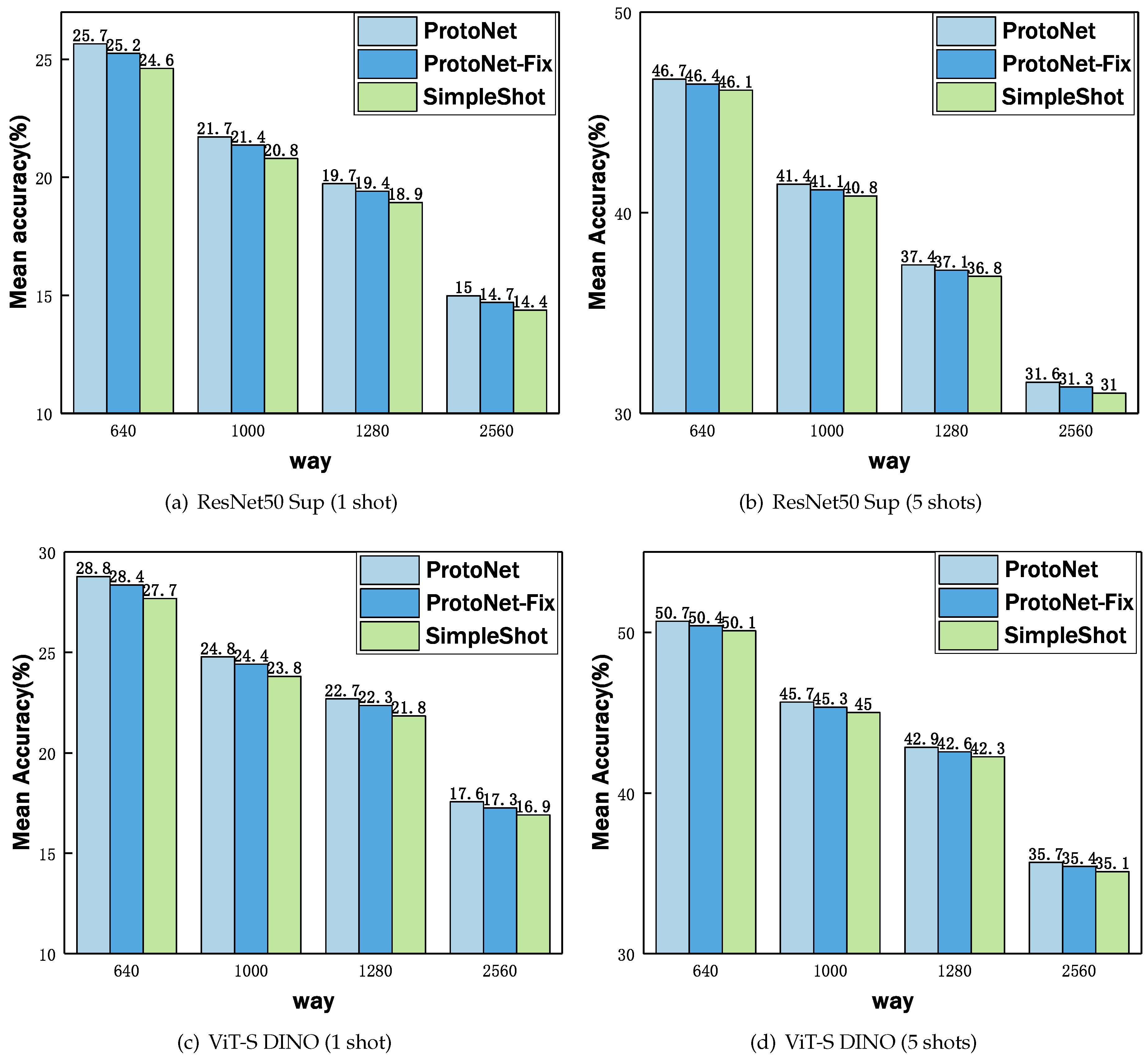
• ProtoNet [35] is widely regarded as a robust task-agnostic embedding baseline model that utilizes support set samples to form prototypes for each class. Classification is performed by computing the distances between query samples and these prototypes. This method notably emphasizes rapid adaptation to new categories without the need for specific task optimization.
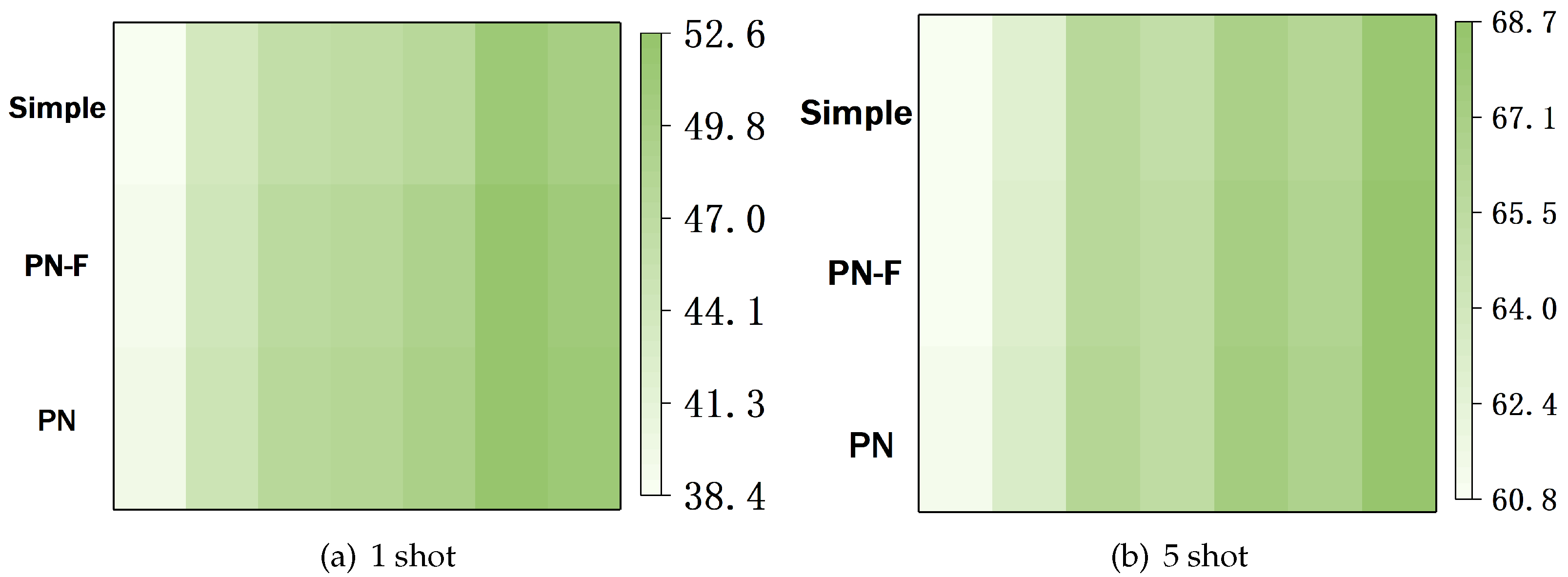
• ProtoNet-Fix, a variant of ProtoNet, fixes the number of classes at five (i.e., 5-way classification) during meta-training, simplifying the training process and enhancing the model’s generalizability post-training. ProtoNet-Fix is employed to assess the impact of different meta-training strategies.
• SimpleShot [21] represents a baseline method for few-shot learning that employs L2 normalization techniques on each sample’s feature vector. Its key feature lies in simplifying the processing flow: it eliminates the need for meta-learning or complex fine-tuning steps. By directly utilizing normalized feature vectors and a nearest-neighbor classifier, SimpleShot achieves impressive performance across multiple few-shot learning tasks.
• Few-shot baseline [3] focuses on optimizing model performance in few-shot settings through fine-tuning. Specifically, it fine-tunes the network backbone using cross-entropy loss applied on the support set to adapt to newly emerged classes. This method is straightforward and effective, particularly suitable for environments with strict label constraints.
• P > M > F [22] employs a cutting-edge method that utilizes ProtoNet for meta-training, building robust class prototype learning mechanisms during the meta-training phase and fine-tuning the meta-traininged backbone through data augmentation techniques in subsequent stages. This strategy not only improves the model’s performance on standard testing tasks but also significantly enhances its adaptability to new domains by extending training data diversity. This method effectively bridges meta-learning and fine-tuning, optimizing the knowledge transfer from base classes to new classes. As SHA-Pipeline also employs data augmentation, P > M > F is replicated within the parallel framework of this study for experimental testing.

The training details for these methods are as follows. To avoid over-engineered training on different datasets and architectures, the experiments adopt a generic training strategy, meta-training the backbone networks from pretrained model checkpoints (for ResNet and ViT). Although this may not yield optimal results in some cases, it simplifies the comparison process. Specifically, meta-training uses an SGD optimizer without weight decay and with a momentum of 0.9, employing a linear learning rate scaling rule [36]: $lr=base\_lr\times \mathrm{way}/5$. The learning rate adjustment uses cosine annealing with five warm-up cycles, gradually increasing from ${10}^{-6}$ to $5\times {10}^{-5}$, then linearly reducing back to ${10}^{-6}$. For ProtoNet, P > M > F, ProtoNet-Fix, and SHA-Pipeline, the backbone networks undergo 100 rounds of meta-training, each comprising 600 few-shot tasks. Note that the number of new classes during meta-training matches those of ProtoNet and P > M > F during meta-testing. Simplifications, including logits scaling [37], mixup [38], and label smoothing [39], are omitted. Early stopping is determined based on validation set performance. For meta-testing of P > M > F, few-shot baseline, and SHA-Pipeline, a fixed learning rate of ${10}^{-6}$ is used for fine-tuning over 50 steps. SHA-Pipeline utilizes the same data augmentation as P > M > F.

5.2. Analysis of Meta-Training Strategy

In this section, we systematically analyze the performance impact of different meta-training strategies on FSL-MNC. We first explore the influence of a fixed-category-number meta-training strategy with five classes on classification accuracy in FSL-MNC. We compare three meta-training strategies: SimpleShot, which involves no meta-training; ProtoNet-Fix, which fixes the number of meta-training classes at five; and ProtoNet, which determines the number of meta-training classes based on the downstream task. As shown in Figure 4, we test the impact of increasing the number of classes from 5 to 2560 (exponentially) on performance across ResNet50, ViT-small, and ViT-base.

Experimental results, as illustrated in Figure 4, reveal a significant impact of meta-training strategies on model performance. Specifically, ProtoNet initially contributes significantly to performance improvement, but its performance advantage diminishes as the number of samples increases from 1 to 5. Notably, even with fewer classes, ProtoNet-Fix significantly enhances performance in a one-sample setting. Figure 5 further showcases the accuracy of these meta-training strategies under various settings, highlighting the good balance ProtoNet-Fix achieves between maintaining high accuracy and reducing computational costs.

Further, extensive experiments are conducted on the ImageNet-MNC dataset to assess how changing meta-training strategies impacts performance across different models and pre-training strategies. Detailed results are summarized in

Table 1. The impact of episodic meta-learning on downstream few-shot learning performance (Imagenet-MNC) under different architecture and pre-training algorithm MetaTr indicates the algorithm used for episodic meta-learning on the corresponding setting (from 5 ways to 2560 ways).

ID	Arch	Pre-Train	MetaTr	Shot	Way											Average
					5	10	20	40	80	160	320	640	1000	1280	2560
1	ResNet50	DINO	-	1	76.78	67.44	58.57	49.84	41.32	33.66	26.85	21.13	17.97	16.48	12.70	38.43
2			-	5	92.74	87.90	82.22	75.54	68.10	60.04	51.98	44.19	39.42	36.83	30.41	60.85
3		Sup.	-	1	84.26	75.54	66.38	57.07	47.75	39.13	31.37	24.62	20.79	18.94	14.37	43.66
4			-	5	94.51	90.36	84.97	78.44	71.04	62.86	54.52	46.11	40.84	36.83	31.01	62.86
5	ViT-small	DINO	-	1	85.34	77.07	68.76	59.87	50.95	42.36	34.65	27.68	23.80	21.84	16.91	46.29
6			-	5	95.20	91.39	86.52	80.50	73.71	66.02	58.09	50.09	45.02	42.25	35.11	65.81
7		Deit	-	1	83.84	76.66	68.87	60.77	52.44	44.00	36.08	28.78	24.55	22.39	17.02	46.85
8			-	5	94.63	91.09	86.41	80.51	73.57	65.71	57.50	49.06	43.54	40.69	33.11	65.07
9	ViT-base	DINO	-	1	86.35	78.80	70.75	62.03	53.08	44.37	36.43	29.20	25.07	23.02	17.80	47.90
10			-	5	95.49	92.16	87.49	81.80	75.16	67.63	59.81	51.82	46.63	43.54	36.57	67.10
11		Deit	-	1	83.28	76.09	68.70	60.99	52.98	44.86	59.04	50.73	25.58	23.42	17.91	51.24
12			-	5	94.50	91.13	86.63	81.10	74.58	67.06	59.04	50.73	45.21	42.67	35.25	66.17
13		MAE	-	1	85.43	78.97	71.98	64.48	56.48	48.10	40.05	32.38	27.78	25.43	19.52	50.05
14			-	5	95.51	92.34	88.35	83.12	76.90	69.56	61.60	53.24	47.63	44.55	37.25	68.19
15	ResNet50	DINO	PN	1	77.62	69.04	60.47	51.29	42.74	34.96	28.02	22.19	18.91	17.28	13.32	39.62
16			PN	5	92.84	88.05	82.44	75.86	68.46	60.45	52.47	44.76	40.02	37.41	30.97	61.25
17		Sup.	PN	1	85.08	77.11	68.24	58.49	49.14	40.40	32.51	25.65	21.72	19.73	14.98	44.82
18			PN	5	94.60	90.51	85.19	78.75	71.38	63.27	54.99	46.66	41.43	37.40	31.55	63.25
19	ViT-small	DINO	PN	1	86.21	78.74	70.74	61.38	52.43	43.73	35.86	28.78	24.78	22.68	17.56	47.54
20			PN	5	95.30	91.55	86.75	80.83	74.08	66.45	58.60	50.68	45.65	42.85	35.69	66.22
21		Deit	PN	1	84.70	78.29	70.81	62.25	53.89	45.33	37.27	29.86	25.51	23.21	17.66	48.07
22			PN	5	94.72	91.25	86.64	80.83	73.93	66.13	58.00	49.64	44.15	41.27	33.68	65.48
23	ViT-base	DINO	PN	1	87.36	80.73	73.05	63.78	54.79	45.95	37.84	30.48	26.21	23.99	18.55	49.34
24			PN	5	95.60	92.34	87.76	82.18	75.59	68.12	60.40	52.51	47.36	44.23	37.24	67.58
25		Deit	PN	1	84.26	77.95	70.92	62.68	54.64	46.38	60.41	51.96	26.68	24.36	18.64	52.63
26			PN	5	94.61	91.31	86.89	81.47	74.99	67.54	59.62	51.39	45.91	43.34	35.90	66.63
27		MAE	PN	1	86.47	80.95	74.33	66.27	58.24	49.72	41.49	33.69	28.94	26.43	20.29	51.53
28			PN	5	95.62	92.54	88.62	83.51	77.34	70.07	62.21	53.94	48.38	45.26	37.94	68.68
29	ResNet50	DINO	PN-F	1	77.62	68.76	59.95	51.18	42.49	34.67	27.67	21.78	18.56	16.97	13.03	39.33
30			PN-F	5	92.84	88.05	82.34	75.72	68.29	60.26	52.24	44.50	39.73	37.14	30.72	61.07
31		Sup.	PN-F	1	85.08	76.83	67.73	58.38	48.90	40.11	32.17	25.25	21.37	19.42	14.70	44.54
32			PN-F	5	94.60	90.51	85.09	78.61	71.22	63.08	54.78	46.41	41.14	37.13	31.31	63.08
33	ViT-small	DINO	PN-F	1	86.21	78.44	70.19	61.27	52.17	43.42	35.50	28.36	24.41	22.35	17.26	47.23
34			PN-F	5	95.30	91.55	86.64	80.68	73.90	66.25	58.37	50.41	45.34	42.57	35.43	66.04
35		Deit	PN-F	1	84.70	78.00	70.27	62.14	53.64	45.03	36.91	29.44	25.14	22.89	17.37	47.78
36			PN-F	5	94.72	91.25	86.53	80.68	73.76	65.93	57.77	49.38	43.85	41.00	33.43	65.30
37	ViT-base	DINO	PN-F	1	87.36	80.38	72.41	63.65	54.50	45.59	37.42	29.98	25.78	23.61	18.21	48.99
38			PN-F	5	95.60	92.34	87.63	82.01	75.38	67.89	60.14	52.19	47.00	43.91	36.94	67.37
39		Deit	PN-F	1	84.26	77.62	70.31	62.56	54.36	46.04	60.00	51.48	26.26	23.99	18.30	52.29
40			PN-F	5	94.61	91.31	86.77	81.30	74.79	67.32	59.36	51.09	45.57	43.03	35.61	66.43
41		MAE	PN-F	1	86.47	80.60	73.68	66.14	57.94	49.35	41.06	33.18	28.50	26.04	19.93	51.17
42			PN-F	5	95.62	92.54	88.49	83.33	77.13	69.83	61.93	53.62	48.01	44.93	37.63	68.46

, showing impressive performance of the SHA-Pipeline even with as few as 5 classes during the meta-testing ranging from 5 to 2560 classes. This demonstrates the effectiveness of the SHA-Pipeline method in handling few-shot learning tasks in FSL-MNC. For instance, in Table 1, the strategy of ProtoNet and ProtoNet-Fix have a closely average accuracy (68.68% and 68.46% in ViT-base with MAE pre-trained).

5.3. Analysis of Computation Overhead

The SHA-Pipeline can be explicitly divided into two phases for analysis: the meta-training phase and the meta-testing phase.

Firstly, the computational overhead during the meta-training phase is analyzed. As shown in Figure 6, our lightweight parallel framework effectively reduces computation time, achieving up to a 150-fold parallel acceleration ratio (when $N=2560$). Additionally, traditional parallel frameworks often face limitations due to exceeding GPU memory capacity when $N>40$, but our framework can smoothly scale meta-training up to $N=2560$.

In the meta-testing phase, the experiment focuses on analyzing the computation time and memory overhead of SHA-Pipeline when handling sets of categories of different sizes. As the number of categories increases, so does the computational demand; however, by employing a lightweight parallel framework, SHA-Pipeline effectively reduces this overhead. Specifically, when the number of categories $N\ge 160$, SHA-Pipeline achieves a super-linear speedup in meta-testing computation time, as shown in Figure 7. This is because the computation time is masked by the time taken to load the dataset into the GPU memory.

Furthermore, the parallel processing of SHA-Pipeline not only optimizes computation time but also significantly reduces memory pressure by efficiently allocating and managing GPU resources. This efficient resource management ensures that the system remains stable even in scenarios with a very large number of categories, avoiding performance bottlenecks due to resource limitations.

The memory overhead of the SHA-Pipeline during the meta-testing phase is illustrated in Figure 8. It is noted that ProtoNet, without the lightweight parallel framework of this experiment, exceeds the 40 G memory limit of a single GPU when the number of categories N surpasses 80. However, the distributed architecture adopted in this experiment effectively mitigates the memory costs associated with larger values of N.

Data from Figure 8 show a consistent upward trend in memory overhead as the number of categories increases. Notably, when N reaches 320, the memory consumption becomes extremely large, exceeding 2560 G, which is significantly beyond the practical operational limits of this experiment (40 G/GPU multiplied by 64 GPUs equals 2560 G), making it challenging to continue the experiment without special measures.

To address this challenge, the experiment further divides the query set into minibatches for forward propagation on each GPU. This approach allows for incremental backward propagation and synchronization updates on these smaller minibatches, effectively reducing memory requirements during training. This strategy not only improves memory utilization efficiency but also ensures that experiments during the meta-testing phase can continue efficiently even with a very large number of categories. The size of these minibatches is 256. Thus, the memory overhead is approximately equal when $N\in 320,640,1000,1280,2560$.

Moreover, this innovative lightweight parallel processing framework not only optimizes memory consumption but also significantly enhances computational efficiency, ensuring stability and high performance for the SHA-Pipeline even in demanding FSL-MNC scenarios. Through this technique, SHA-Pipeline not only addresses the issue of high memory costs but also enhances the model’s scalability and flexibility when handling large datasets, providing robust support for broader practical applications in the future.

5.4. FSL-MNC Performance

This experiment included a detailed evaluation of the few-shot generalization capabilities of SHA-Pipeline in FSL-MNC scenarios. In this experiment, SHA-Pipeline utilized a fixed number of categories ($N=5$) for ProtoNet’s meta-traininging to ensure training consistency and reduce the model’s sensitivity to the number of categories. This approach aimed to test the model’s learning efficiency and generalization capabilities under conditions with fewer categories.

The core architecture for all methods employed the DINO pre-trained ViT-small backbone network. The choice of the DINO pre-trained model was due to its exceptional ability in handling image feature extraction, particularly in image understanding and representation learning. This high-performance backbone network provided SHA-Pipeline with robust visual information processing capabilities, making it more suitable for complex few-shot learning tasks.

Table 2. Performance on ImageNet-MNC (under different numbers of ways) in comparison with other FSL algorithms.

Method	Shot	Way											Average
		5	10	20	40	80	160	320	640	1000	1280	2560
ProtoNet	1	86.21	78.74	70.74	61.38	52.43	43.73	35.86	28.78	24.78	22.68	17.56	47.54
	5	95.30	91.55	86.75	80.83	74.08	66.45	58.60	50.68	45.65	42.85	35.69	66.22
ProtoNet-Fix	1	86.21	78.44	70.19	61.27	52.17	43.42	35.50	28.3555	24.41	22.35	17.26	47.23
	5	95.30	91.55	86.64	80.68	73.90	66.25	58.37	50.41	45.34	42.57	35.43	66.04
SimpleShot	1	85.34	77.07	68.76	59.87	50.95	42.36	34.65	27.68	23.80	21.84	16.91	46.29
	5	95.20	91.39	86.52	80.50	73.71	66.02	58.09	50.09	45.02	42.25	35.11	65.81
few-shot-baseline	1	86.21	78.59	70.47	61.32	52.30	43.57	35.77	28.68	24.68	22.60	17.49	47.43
	5	95.30	91.55	86.70	80.75	73.99	66.35	58.54	50.61	45.57	42.78	35.62	66.16
P > M > F	1	86.82	79.91	72.13	62.81	53.83	45.02	37.02	29.83	25.71	23.48	18.18	48.61
	5	95.78	92.49	87.86	81.97	75.20	67.49	59.53	51.52	46.40	43.49	36.18	67.08
SHA-Pipeline (CPCC)	1	88.24	81.59	73.60	64.25	55.31	46.38	38.23	30.98	26.83	24.40	19.02	49.89
	5	97.06	94.00	89.18	83.27	76.54	68.71	60.62	52.55	47.41	44.32	36.93	68.24
SHA-Pipeline (Triplet Loss)	1	89.74	82.01	73.49	63.35	53.82	44.75	36.80	29.88	26.08	23.85	18.91	49.33
	5	97.63	94.30	89.29	83.26	76.68	69.03	61.21	52.88	47.90	44.89	37.25	68.57

displays the average accuracy results obtained through different methods. These results not only showcase the performance of SHA-Pipeline in FSL-MNC scenarios but also compare the performance of other methods under the same conditions, offering a comprehensive performance assessment. This comparison clearly illustrates SHA-Pipeline’s advantages in generalization capability and adaptation to new categories, as well as its ability to maintain stable performance in FSL-MNC environments. Additionally, these results validate the effectiveness of the fixed category number meta-traininging strategy in practical applications, providing important insights and guidance for future few-shot learning research.

From Table 2, it is observed that the SHA-Pipeline method achieved the highest average accuracy across various category configurations. Particularly, in the setting with one sample per class, SHA-Pipeline’s average accuracy reached 49.89%, which is 1.28% higher than its closest competitor, P > M > F. This indicates that under more stringent few-shot conditions, SHA-Pipeline more effectively utilizes its category hierarchy fine-tuning mechanism to improve classification performance.

In the experimental setting with five samples per class, SHA-Pipeline’s average accuracy even reached 68.24%, which is 1.16% higher than P > M > F, demonstrating its excellent performance when handling slightly more sample data. This performance enhancement is particularly noticeable as the number of categories increases, confirming that SHA-Pipeline is not only adaptable but also maintains stable performance under high-pressure FSL-MNC scenarios.

Moreover, comparing results from different methods, it can be seen that SHA-Pipeline’s gap with other methods becomes more pronounced in settings with more categories (such as 5-way and 10-way), possibly due to its unique category hierarchy and fine-tuning strategy being most effective when category information is more concentrated. Even when category numbers reach a massive scale (like 2560-way), although performance declines for all methods, the decline is relatively smaller for SHA-Pipeline, further proving its superior generalization capabilities and adaptability to complex classification environments.

Overall, these data not only demonstrate the advantages of SHA-Pipeline in FSL-MNC scenarios but also highlight its ability to maintain consistent performance across different sample densities. This stability and excellence in performance provide significant experimental evidence and theoretical support for the field of few-shot learning, aiding in further development and application of related technologies.

Figure 9 further illustrates the average accuracy trends across all methods in settings with 1 and 5 samples per class, as category numbers change. Notably, SHA-Pipeline consistently provides higher classification accuracy than other methods across all tested category settings, including scenarios with fewer categories.

5.5. Standard Benchmark Performance

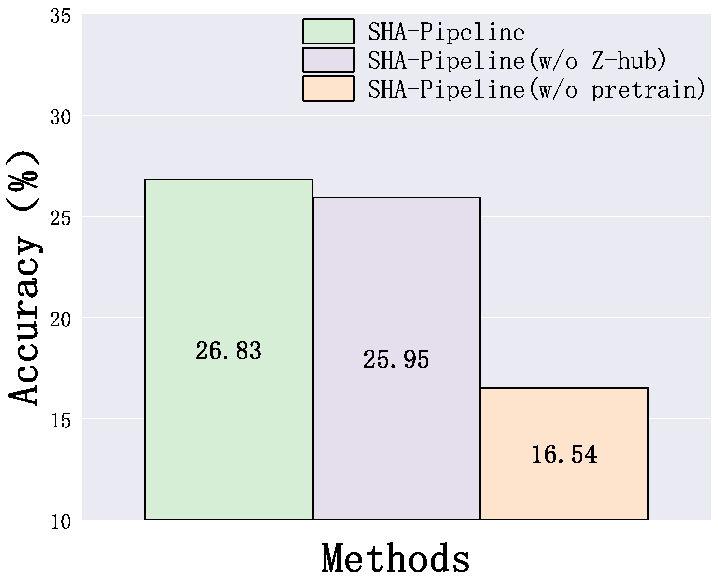
Due to SHA-Pipeline utilizing more advanced backbone networks and additional external data, the results of this experiment are not directly comparable with many previous state-of-the-art (SOTA) algorithms. This comparison is intended to explore the effects of simple improvements, such as upgrading the feature backbone to modern network architectures and leveraging publicly available data for large-scale pretraining, against the intensive research on few-shot learning (FSL) algorithms over the past five years. As shown in

Table 3. Comparison with represen tative SOTA FSL algorithms. Methods using external data and/or labels are marked.

Method (Backbone)	External	External	CIFAR-FS		MiniImageNet
	Data	Label	5w1s	5w5s	5w1s	5w5s
Inductive
ProtoNet (CNN-4-64) [35]			49.4	68.2	55.5	72.0
Baseline++ (CNN-4-64) [40]					48.2	66.4
MetaOpt-SVM (ResNet12) [41]			72.0	84.3	61.4	77.9
Meta-Baseline (ResNet12) [42]					68.6	83.7
RS-FSL (ResNet12) [43]		✓			65.3
Transductive
Fine-tuning (WRN-28-10) [3]			76.6	85.8	65.7	78.4
SIB (WRN-28-10) [44]			80.0	85.3	70.0	79.2
PT-MAP (WRN-28-10) [45]			87.7	90.7	82.9	88.8
CNAPS + FETI (ResNet18) [46]	✓	✓			79.9	91.5
Self-supervised
ProtoNet (WRN-28-10) [47]			73.6	86.1	62.9	79.9
ProtoNet (AMDIM ResNet) [48]	✓				76.8	91.0
EPNet + SSL (WRN-28-10) [49]	✓				79.2	88.1
Semi-supervised
LST (ResNet12) [50]	✓				70.1	78.7
PLCM (ResNet12) [51]	✓		77.6	86.1	70.1	83.7
ProtoNet (IN1K, IN1K, ViT-Small)	✓		80.7	91.8	92.5	97.7
SimpleShot (IN1K, ViT-Small)	✓		80.3	92.1	92.8	97.2
few-shot-baseline (IN1K, ViT-Small)	✓		80.9	91.9	92.7	97.4
P > M > F (IN1K, ViT-Small)	✓		81.1	92.5	92.7	98.0
SHA-Pipeline (IN1K, ViT-Small, CPCC)	✓		81.9	93.4	93.6	98.9

, the single-domain case results, including miniImageNet and CIFAR-FS, as well as the cross-domain dataset results in Meta-Dataset (

Table 4. Comparison with SOTA FSL algorithms on Meta-Dataset.

Training Dataset = ImageNet	In-Domian	Cross-Domian
	INet	Omglot	Acraft	CUB	DTD	QDraw	Fungi	Flower	Sign	COCO	Avg Acc (%)
ProtoNet [28] (RN18)	50.5	59.9	53.1	68.7	66.5	48.9	39.7	85.2	47.1	41.0	56.1
ALFA+FP-MAML [52] (RN12)	52.8	61.8	63.4	69.7	70.7	59.1	41.4	85.9	60.7	48.1	61.4
BOHB [53] (RN18)	51.9	67.5	54.1	70.6	68.3	50.3	41.3	87.3	51.8	48.0	59.1
CTX [29] (RN34)	62.7	82.2	79.4	80.6	75.5	72.6	51.8	95.3	82.6	59.9	74.2
ProtoNet (DINO/IN1K, ViT-small)	74.3	80.3	76.0	84.2	84.9	69.8	54.2	93.6	87.9	62.3	76.8
SimpleShot (DINO/IN1K, ViT-small)	73.2	79.1	76.4	84.6	85.8	70.5	53.7	92.7	87.4	61.9	76.5
few-shot-baseline (DINO/IN1K, ViT-small)	74.3	80.3	75.6	83.8	86.6	71.2	54.8	94.6	87.0	61.6	77.0
P > M > F (DINO/IN1K, ViT-small)	74.7	80.7	76.8	85.0	86.6	71.3	54.8	94.6	88.3	62.6	77.5
SHA-Pipeline (DINO/IN1K, ViT-small, CPCC)	75.4	81.5	77.5	85.9	87.5	72.0	55.3	95.2	89.2	63.2	78.3

) demonstrate that despite its relatively simple framework, SHA-Pipeline surpasses the latest techniques in both intra-domain and cross-domain conditions. This underscores the efficiency and applicability of the SHA-Pipeline method.

Specifically, on miniImageNet and CIFAR-FS, SHA-Pipeline achieved 5-way 5-shot accuracies of 91.8% and 93.4%, respectively, markedly higher than other methods such as ProtoNet and MetaOpt-SVM. Within the diverse categories of the Meta-Dataset, SHA-Pipeline also excelled, achieving accuracies of 95.5% and 89.2% in the Flower and Sign categories, showcasing its robust generalization capabilities when dealing with diverse and complex datasets. Additionally, compared to other algorithms using traditional models or techniques, SHA-Pipeline also exhibited significant advantages in resource utilization and computational efficiency.

In the single-source benchmark tests presented in Table 3, some competitors also used external data or ImageNet pretraining to boost performance. However, the advantage displayed by SHA-Pipeline in Table 4, particularly in surpassing purely external self-supervised SOTA methods in cross-domain few-shot learning competitions, validates that even in extremely few-shot settings, SHA-Pipeline maintains exceptional performance. These results highlight the efficacy of standard cross-entropy pretraining on large network models and nearest neighbor searches based on support sets in the current field of few-shot learning, consistent with recent literature observations that for large network models, simple yet powerful pretraining combined with fine-tuned nearest neighbor searches suffices to address most few-shot learning challenges.

These superior performance metrics are partly due to the advanced backbone networks and external data used by SHA-Pipeline. Compared to other classical few-shot learning algorithms, SHA-Pipeline’s design and implementation offer several key improvements: (1) ProtoNet builds on forming class prototypes, which excel in quickly adapting to new categories but may not capture all necessary intra-class variations in cases with a very large number of categories or highly diverse datasets. (2) SimpleShot simplifies the classification process through L2 normalization of feature vectors, performing well in some scenarios but lacking adaptability to complex or highly nonlinear data structures. (3) The Few-shot Baseline focuses on optimizing few-shot performance through fine-tuning, a direct and effective approach, but it typically relies on the quality of initial pretraining and sensitivity to specific tasks. (4) The P > M > F method enhances adaptability by adding subsequent fine-tuning steps on top of ProtoNet. Although it improves performance, it still heavily depends on the quality of features learned during the initial meta-learning phase.

In contrast, SHA-Pipeline, by integrating more external data and employing the efficient ViT-Small backbone network, not only optimizes the quality of feature learning but also significantly reduces memory and computational overhead through its unique partitioning and incremental learning strategies. This allows SHA-Pipeline to maintain high performance while also greatly enhancing operational efficiency and scalability. For example, in experiments on CIFAR-FS and miniImageNet, SHA-Pipeline exceeded other methods by at least 1% in the 5-way 5-shot setting, and in handling multiple domains in the Meta-Dataset, it surpassed the nearest competitor by at least 1.1%, demonstrating its robustness and adaptability across various settings.

These findings emphasize the importance of selecting and optimizing backbone networks and training strategies when designing few-shot learning algorithms. With the evolution of network architectures and training methods, the future of few-shot learning is anticipated to focus more on improving generalization capabilities and handling complexity through more effective data utilization and algorithmic innovations. The successful implementation of SHA-Pipeline offers a viable path for future research, especially in scenarios dealing with large-scale and diverse datasets.

5.6. Ablation Study

This experiment’s ablation study focuses on examining the impact of Z-score normalization and the role of pretraining strategies within the SHA-Pipeline. The study was conducted by excluding the Z-score normalization step from these methods and analyzing its impact on performance. Subsequently, the scenario where the backbone network is trained from scratch during the meta-training phase, omitting pretraining, was explored. Experimental results are displayed in Figure 10.

Impact of Z-Score Normalization

Notably, Figure 10 shows that the accuracy drops by approximately 0.9% when the Z-score normalization step is removed. This finding emphasizes the significance of Z-score normalization as a key element in SHA-Pipeline. The Z-score normalization step significantly contributes to addressing hubness-related issues, enhancing the quality of hierarchical clustering and subsequently improving performance.

Impact of Pretraining

Figure 10 reveals a substantial performance decline of over 10% when pretraining is omitted. In other words, the accuracy experiences a significant drop when meta-training is conducted without the benefits of pretraining. This result underscores the crucial role of pretraining in enhancing the initial state of the backbone network before starting meta-training. It highlights that the pretraining phase plays a key role in setting a solid foundation for subsequent meta-training operations, ultimately aiding in enhancing overall performance.

Specifically, the second part of Figure 10 demonstrates the performance changes after the omission of the pretraining step. It is clear that the absence of pretraining leads to a significant decrease in accuracy. This further validates the importance of pretraining in few-shot learning, providing the model with better initial parameters, thus significantly enhancing the effectiveness of meta-training and the final classification performance.

Through these ablation studies, we can better understand the critical roles of Z-score normalization and pretraining in SHA-Pipeline, offering valuable insights for further optimization of few-shot learning algorithms.

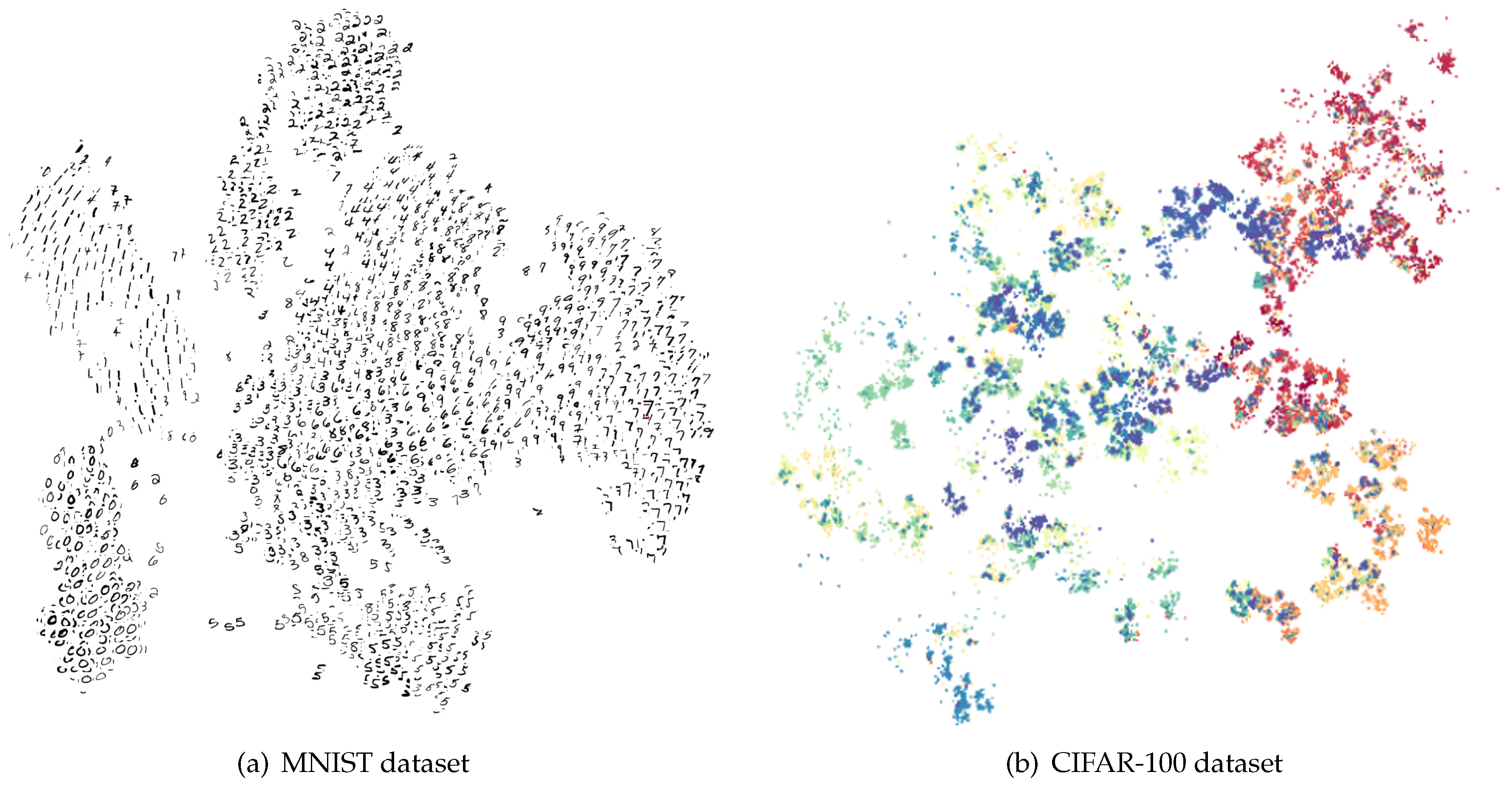
5.7. Visualization Study

On the MNIST and CIFAR-100 datasets, this study applied t-SNE to reduce and visualize image features. The image features were reduced to a two-dimensional space and projected using t-SNE for display purposes.

From Figure 11a, it is evident that different categories of digits are projected into distinct regions. Digits of the same category (i.e., points representing the same character) mostly cluster together, forming clear clusters. There are distinct boundaries between clusters, indicating that the feature vectors can effectively differentiate between categories. The clustering effect demonstrates that the model’s extracted features possess good discriminative power, with digits from different categories well-separated, reflecting the representativeness and effectiveness of the feature vectors in classification.

The CIFAR-100 dataset is more complex, containing more categories and higher image complexity, including labels at different levels of granularity. The CIFAR-100 dataset consists of 20 superclasses encompassing a total of 100 subclasses, with each image labeled with both coarse- and fine-grained categories. From Figure 11b, images of different categories are projected into distinct color areas, each color representing a different level of hierarchical clustering. Similar to the MNIST dataset, images of the same superclass (i.e., points of the same color) also cluster together. However, due to the complexity of the CIFAR-100 dataset, the clustering boundaries are not as clear as those in the MNIST dataset. Despite the more dispersed distribution of feature vectors due to the dataset’s greater number of categories and more complex image backgrounds, an overall clustering effect is still observable. The clustering effect is slightly blurred, but the overall trend still reflects the distinctions between categories. Notably, in the CIFAR-100 dataset, different colors represent different hierarchical clustering results, indicating that the model captures the hierarchical structure among categories effectively. This suggests that SHA-Pipeline’s clustering algorithm helps the model better understand and utilize the relationships between categories, thereby enhancing classification performance.

Through the visualization of features from the MNIST and CIFAR-100 datasets, the following conclusions can be drawn: the visualization results after t-SNE projection demonstrate that the model’s extracted features perform well in distinguishing between different categories, particularly evident in the MNIST dataset. Due to the diversity of categories and complexity of images, the clustering effect in CIFAR-100 is slightly inferior to that in the MNIST dataset, but clear category clustering effects are still evident. The visualization results across different datasets showcase the model’s feature extraction capabilities in handling both simple and complex datasets, validating the model’s generalizability and robustness. These visual results not only confirm the effectiveness of the model in few-shot learning tasks but also provide important references for further optimization of the model.

6. Conclusions and Future Work

We introduced a new problem named few-shot learning with many novel classes (FSL-MNC) which encourages the exploration of few-shot learning frameworks in real-world scenarios characterized by a large diversity of classes. This scenario presents significant computational and generalization challenges. In addressing FSL-MNC, we demonstrated that meta-training with a fixed number of ways provides a practical compromise between computational overhead and predictive performance. Notably, when handling a large number of classes, effectively extracting and utilizing the class hierarchy structure was shown to substantially enhance performance. Additionally, we developed a lightweight distributed framework specifically tailored for FSL-MNC, enabling a robust comparison against established baselines. Our evaluations confirm that the proposed SHA-Pipeline delivers exceptionally competitive performance in FSL-MNC contexts.

Limitations and Future Work. Our investigation predominantly centered on image data, without integrating textual information, which could provide additional context and improve model robustness and applicability in FSL-MNC. Future research could explore multimodal approaches that combine both visual and textual data, potentially enhancing performance in complex real-life applications such as visual tracking [54,55]. Furthermore, our current implementation of SHA-Pipeline, while effective, is somewhat basic in its integration with meta-training techniques. Investigating more advanced meta-training strategies could lead to further enhancements in performance. Additionally, the computational demands of SHA-Pipeline, particularly during the meta-testing phase, pose a challenge. Future efforts should aim to optimize the computational efficiency of the pipeline during the fine-tuning stages, potentially reducing runtime and resource consumption without sacrificing accuracy.

References

1. An, Y.; Xue, H.; Zhao, X.; Wang, J. From Instance to Metric Calibration: A Unified Framework for Open-World Few-Shot Learning. IEEE Trans. Pattern Anal. Mach. Intell. 2023, 45, 9757–9773. [Google Scholar] [CrossRef] [PubMed]
2. Wang, Y.; Yao, Q.; Kwok, J.T.; Ni, L.M. Generalizing from a Few Examples: A Survey on Few-shot Learning. ACM Comput. Surv. 2021, 53, 63:1–63:34. [Google Scholar] [CrossRef]
3. Dhillon, G.S.; Chaudhari, P.; Ravichandran, A.; Soatto, S. A Baseline for Few-Shot Image Classification. In Proceedings of the 8th International Conference on Learning Representations, ICLR 2020, Addis Ababa, Ethiopia, 26–30 April 2020; OpenReview.net: Addis Ababa, Ethiopia, 2020. [Google Scholar]
4. Lin, Z.; Yang, W.; Wang, H.; Chi, H.; Lan, L.; Wang, J. Scaling Few-Shot Learning for the Open World. In Proceedings of the AAAI Conference on Artificial Intelligence, Vancouver, BC, Canada, 20–27 February 2024; Volume 38, pp. 13846–13854. [Google Scholar]
5. Willes, J.; Harrison, J.; Harakeh, A.; Finn, C.; Pavone, M.; Waslander, S. Bayesian embeddings for few-shot open world recognition. IEEE Trans. Pattern Anal. Mach. Intell. 2022, 46, 1513–1529. [Google Scholar] [CrossRef] [PubMed]
6. Parmar, J.; Chouhan, S.S.; Raychoudhury, V.; Rathore, S.S. Open-world Machine Learning: Applications, Challenges, and Opportunities. ACM Comput. Surv. 2023, 55, 205:1–205:37. [Google Scholar] [CrossRef]
7. Russakovsky, O.; Deng, J.; Su, H.; Krause, J.; Satheesh, S.; Ma, S.; Huang, Z.; Karpathy, A.; Khosla, A.; Bernstein, M.S.; et al. ImageNet Large Scale Visual Recognition Challenge. Int. J. Comput. Vis. 2015, 115, 211–252. [Google Scholar] [CrossRef]
8. Deng, J.; Dong, W.; Socher, R.; Li, L.; Li, K.; Fei-Fei, L. ImageNet: A large-scale hierarchical image database. In Proceedings of the 2009 IEEE Computer Society Conference on Computer Vision and Pattern Recognition (CVPR 2009), Miami, FL, USA, 20–25 June 2009; IEEE Computer Society: Washington, DC, USA, 2009; pp. 248–255. [Google Scholar] [CrossRef]
9. Baz, A.E.; Ullah, I.; Alcobaça, E.; de Carvalho, A.C.P.L.F.; Chen, H.; Ferreira, F.; Gouk, H.; Guan, C.; Guyon, I.; Hospedales, T.M.; et al. Lessons learned from the NeurIPS 2021 MetaDL challenge: Backbone fine-tuning without episodic meta-learning dominates for few-shot learning image classification. In Proceedings of the NeurIPS 2021 Competitions and Demonstrations Track, Online, 6–14 December 2021; Kiela, D., Ciccone, M., Caputo, B., Eds.; Proceedings of Machine Learning Research (PMLR): London, UK, 2021; Volume 176, pp. 80–96. [Google Scholar]
10. Rajeswaran, A.; Finn, C.; Kakade, S.M.; Levine, S. Meta-Learning with Implicit Gradients. In Proceedings of the Advances in Neural Information Processing Systems 32: Annual Conference on Neural Information Processing Systems 2019, NeurIPS 2019, Vancouver, BC, Canada, 8–14 December 2019; pp. 113–124. [Google Scholar]
11. Silla, C.N.; Freitas, A.A. A survey of hierarchical classification across different application domains. Data Min. Knowl. Discov. 2011, 22, 31–72. [Google Scholar] [CrossRef]
12. Novack, Z.; McAuley, J.; Lipton, Z.C.; Garg, S. Chils: Zero-shot image classification with hierarchical label sets. In Proceedings of the International Conference on Machine Learning, Honolulu, HI, USA, 23–29 July 2023; PMLR: London, UK, 2023; pp. 26342–26362. [Google Scholar]
13. Guo, Y.; Xu, M.; Li, J.; Ni, B.; Zhu, X.; Sun, Z.; Xu, Y. Hcsc: Hierarchical contrastive selective coding. In Proceedings of the IEEE/CVF Conference on Computer Vision and Pattern Recognition, New Orleans, LA, USA, 18–24 June 2022; pp. 9706–9715. [Google Scholar]
14. Hospedales, T.M.; Antoniou, A.; Micaelli, P.; Storkey, A.J. Meta-Learning in Neural Networks: A Survey. IEEE Trans. Pattern Anal. Mach. Intell. 2022, 44, 5149–5169. [Google Scholar] [CrossRef] [PubMed]
15. Vinyals, O.; Blundell, C.; Lillicrap, T.; Kavukcuoglu, K.; Wierstra, D. Matching Networks for One Shot Learning. In Proceedings of the Advances in Neural Information Processing Systems 29: Annual Conference on Neural Information Processing Systems 2016, Barcelona, Spain, 5–10 December 2016; pp. 3630–3638. [Google Scholar]
16. Ravi, S.; Larochelle, H. Optimization as a Model for Few-Shot Learning. In Proceedings of the 5th International Conference on Learning Representations, ICLR 2017, Toulon, France, 24–26 April 2017; Conference Track Proceedings. OpenReview.net: Toulon, France, 2017. [Google Scholar]
17. Ye, H.; Hu, H.; Zhan, D.; Sha, F. Few-Shot Learning via Embedding Adaptation with Set-to-Set Functions. In Proceedings of the 2020 IEEE/CVF Conference on Computer Vision and Pattern Recognition, CVPR 2020, Seattle, WA, USA, 13–19 June 2020; Computer Vision Foundation: New York, NY, USA; IEEE: Piscataway, NJ, USA, 2020; pp. 8805–8814. [Google Scholar] [CrossRef]
18. Ye, H.; Chao, W. How to Train Your MAML to Excel in Few-Shot Classification. In Proceedings of the Tenth International Conference on Learning Representations, ICLR 2022, Virtual Event, 25–29 April 2022. [Google Scholar]
19. Geng, C.; Huang, S.; Chen, S. Recent Advances in Open Set Recognition: A Survey. IEEE Trans. Pattern Anal. Mach. Intell. 2021, 43, 3614–3631. [Google Scholar] [CrossRef]
20. Finn, C.; Abbeel, P.; Levine, S. Model-Agnostic Meta-Learning for Fast Adaptation of Deep Networks. In Proceedings of the 34th International Conference on Machine Learning, ICML 2017, Sydney, NSW, Australia, 6–11 August 2017; Precup, D., Teh, Y.W., Eds.; Proceedings of Machine Learning Research (PMLR): London, UK, 2017; Volume 70, pp. 1126–1135. [Google Scholar]
21. Wang, Y.; Chao, W.; Weinberger, K.Q.; van der Maaten, L. SimpleShot: Revisiting Nearest-Neighbor Classification for Few-Shot Learning. arXiv 2019, arXiv:1911.04623. [Google Scholar] [CrossRef]
22. Hu, S.X.; Li, D.; Stühmer, J.; Kim, M.; Hospedales, T.M. Pushing the Limits of Simple Pipelines for Few-Shot Learning: External Data and Fine-Tuning Make a Difference. In Proceedings of the IEEE/CVF Conference on Computer Vision and Pattern Recognition, CVPR 2022, New Orleans, LA, USA, 18–24 June 2022; IEEE: Piscataway, NJ, USA, 2022; pp. 9058–9067. [Google Scholar] [CrossRef]
23. Liu, L.; Zhou, T.; Long, G.; Jiang, J.; Zhang, C. Many-Class Few-Shot Learning on Multi-Granularity Class Hierarchy. IEEE Trans. Knowl. Data Eng. 2022, 34, 2293–2305. [Google Scholar] [CrossRef]
24. Li, A.; Luo, T.; Lu, Z.; Xiang, T.; Wang, L. Large-Scale Few-Shot Learning: Knowledge Transfer with Class Hierarchy. In Proceedings of the IEEE Conference on Computer Vision and Pattern Recognition, CVPR 2019, Long Beach, CA, USA, 16–20 June 2019; Computer Vision Foundation: New York, NY, USA; IEEE: Piscataway, NJ, USA, 2019; pp. 7212–7220. [Google Scholar] [CrossRef]
25. Sarfraz, M.S.; Sharma, V.; Stiefelhagen, R. Efficient Parameter-Free Clustering Using First Neighbor Relations. In Proceedings of the IEEE Conference on Computer Vision and Pattern Recognition, CVPR 2019, Long Beach, CA, USA, 16–20 June 2019; Computer Vision Foundation: New York, NY, USA; IEEE: Piscataway, NJ, USA, 2019; pp. 8934–8943. [Google Scholar] [CrossRef]
26. Fei, N.; Gao, Y.; Lu, Z.; Xiang, T. Z-Score Normalization, Hubness, and Few-Shot Learning. In Proceedings of the 2021 IEEE/CVF International Conference on Computer Vision, ICCV 2021, Montreal, QC, Canada, 10–17 October 2021; IEEE: Piscataway, NJ, USA, 2021; pp. 142–151. [Google Scholar] [CrossRef]
27. Bertinetto, L.; Henriques, J.F.; Torr, P.H.S.; Vedaldi, A. Meta-learning with differentiable closed-form solvers. In Proceedings of the 7th International Conference on Learning Representations, ICLR 2019, New Orleans, LA, USA, 6–9 May 2019. [Google Scholar]
28. Triantafillou, E.; Zhu, T.; Dumoulin, V.; Lamblin, P.; Evci, U.; Xu, K.; Goroshin, R.; Gelada, C.; Swersky, K.; Manzagol, P.; et al. Meta-Dataset: A Dataset of Datasets for Learning to Learn from Few Examples. In Proceedings of the 8th International Conference on Learning Representations, ICLR 2020, Addis Ababa, Ethiopia, 26–30 April 2020. [Google Scholar]
29. Doersch, C.; Gupta, A.; Zisserman, A. CrossTransformers: Spatially-aware few-shot transfer. In Proceedings of the Advances in Neural Information Processing Systems 33: Annual Conference on Neural Information Processing Systems 2020, NeurIPS 2020, Virtual, 6–12 December 2020. [Google Scholar]
30. Dosovitskiy, A.; Beyer, L.; Kolesnikov, A.; Weissenborn, D.; Zhai, X.; Unterthiner, T.; Dehghani, M.; Minderer, M.; Heigold, G.; Gelly, S.; et al. An Image is Worth 16×16 Words: Transformers for Image Recognition at Scale. In Proceedings of the 9th International Conference on Learning Representations, ICLR 2021, Virtual Event, Austria, 3–7 May 2021. [Google Scholar]
31. He, K.; Zhang, X.; Ren, S.; Sun, J. Deep Residual Learning for Image Recognition. In Proceedings of the 2016 IEEE Conference on Computer Vision and Pattern Recognition, CVPR 2016, Las Vegas, NV, USA, 27–30 June 2016; IEEE Computer Society: Piscataway, NJ, USA, 2016; pp. 770–778. [Google Scholar] [CrossRef]
32. Caron, M.; Touvron, H.; Misra, I.; Jégou, H.; Mairal, J.; Bojanowski, P.; Joulin, A. Emerging Properties in Self-Supervised Vision Transformers. In Proceedings of the 2021 IEEE/CVF International Conference on Computer Vision, ICCV 2021, Montreal, QC, Canada, 10–17 October 2021; IEEE: Piscataway, NJ, USA, 2021; pp. 9630–9640. [Google Scholar] [CrossRef]
33. Touvron, H.; Cord, M.; Douze, M.; Massa, F.; Sablayrolles, A.; Jégou, H. Training data-efficient image transformers & distillation through attention. In Proceedings of the 38th International Conference on Machine Learning, ICML 2021; Virtual Event, 18–24 July 2021, Meila, M., Zhang, T., Eds.; Proceedings of Machine Learning Research (PMLR): London, UK, 2021; Volume 139, pp. 10347–10357. [Google Scholar]
34. He, K.; Chen, X.; Xie, S.; Li, Y.; Dollár, P.; Girshick, R.B. Masked Autoencoders Are Scalable Vision Learners. In Proceedings of the IEEE/CVF Conference on Computer Vision and Pattern Recognition, CVPR 2022, New Orleans, LA, USA, 18–24 June 2022; IEEE: Piscataway, NJ, USA, 2022; pp. 15979–15988. [Google Scholar] [CrossRef]
35. Snell, J.; Swersky, K.; Zemel, R.S. Prototypical Networks for Few-shot Learning. In Proceedings of the Advances in Neural Information Processing Systems 30: Annual Conference on Neural Information Processing Systems 2017, Long Beach, CA, USA, 4–9 December 2017; pp. 4077–4087. [Google Scholar]
36. Goyal, P.; Dollár, P.; Girshick, R.B.; Noordhuis, P.; Wesolowski, L.; Kyrola, A.; Tulloch, A.; Jia, Y.; He, K. Accurate, Large Minibatch SGD: Training ImageNet in 1 Hour. arXiv 2017, arXiv:1706.02677. [Google Scholar] [CrossRef]
37. Oreshkin, B.N.; López, P.R.; Lacoste, A. TADAM: Task dependent adaptive metric for improved few-shot learning. In Proceedings of the Advances in Neural Information Processing Systems 31: Annual Conference on Neural Information Processing Systems 2018, NeurIPS 2018, Montréal, QC, Canada, 3–8 December 2018; pp. 719–729. [Google Scholar]
38. Zhang, H.; Cissé, M.; Dauphin, Y.N.; Lopez-Paz, D. mixup: Beyond Empirical Risk Minimization. In Proceedings of the 6th International Conference on Learning Representations, ICLR 2018, Vancouver, BC, Canada, 30 April–3 May 2018. Conference Track Proceedings. [Google Scholar]
39. Szegedy, C.; Vanhoucke, V.; Ioffe, S.; Shlens, J.; Wojna, Z. Rethinking the Inception Architecture for Computer Vision. In Proceedings of the 2016 IEEE Conference on Computer Vision and Pattern Recognition, CVPR 2016, Las Vegas, NV, USA, 27–30 June 2016; IEEE Computer Society: Piscataway, NJ, USA, 2016; pp. 2818–2826. [Google Scholar] [CrossRef]
40. Chen, W.; Liu, Y.; Kira, Z.; Wang, Y.F.; Huang, J. A Closer Look at Few-shot Classification. In Proceedings of the 7th International Conference on Learning Representations, ICLR 2019, New Orleans, LA, USA, 6–9 May 2019. [Google Scholar]
41. Lee, K.; Maji, S.; Ravichandran, A.; Soatto, S. Meta-Learning With Differentiable Convex Optimization. In Proceedings of the IEEE Conference on Computer Vision and Pattern Recognition, CVPR 2019, Long Beach, CA, USA, 16–20 June 2019; Computer Vision Foundation: New York, NY, USA; IEEE: Piscataway, NJ, USA, 2019; pp. 10657–10665. [Google Scholar] [CrossRef]
42. Chen, Y.; Liu, Z.; Xu, H.; Darrell, T.; Wang, X. Meta-Baseline: Exploring Simple Meta-Learning for Few-Shot Learning. In Proceedings of the 2021 IEEE/CVF International Conference on Computer Vision, ICCV 2021, Montreal, QC, Canada, 10–17 October 2021; IEEE: Piscataway, NJ, USA, 2021; pp. 9042–9051. [Google Scholar] [CrossRef]
43. Afham, M.; Khan, S.; Khan, M.H.; Naseer, M.; Khan, F.S. Rich Semantics Improve Few-Shot Learning. In Proceedings of the 32nd British Machine Vision Conference 2021, BMVC 2021, Online, 22–25 November 2021; BMVA Press: Durham, UK, 2021; p. 152. [Google Scholar]
44. Hu, S.X.; Moreno, P.G.; Xiao, Y.; Shen, X.; Obozinski, G.; Lawrence, N.D.; Damianou, A.C. Empirical Bayes Transductive Meta-Learning with Synthetic Gradients. In Proceedings of the 8th International Conference on Learning Representations, ICLR 2020, Addis Ababa, Ethiopia, 26–30 April 2020. [Google Scholar]
45. Hu, Y.; Gripon, V.; Pateux, S. Leveraging the Feature Distribution in Transfer-Based Few-Shot Learning. In Proceedings of the Artificial Neural Networks and Machine Learning-ICANN 2021-30th International Conference on Artificial Neural Networks, Bratislava, Slovakia, 14–17 September 2021; Proceedings, Part II. Farkas, I., Masulli, P., Otte, S., Wermter, S., Eds.; Springer: Cham, Switzerland, 2021; Volume 12892, pp. 487–499, Lecture Notes in Computer Science. [Google Scholar] [CrossRef]
46. Bateni, P.; Barber, J.; van de Meent, J.; Wood, F. Enhancing Few-Shot Image Classification with Unlabelled Examples. In Proceedings of the IEEE/CVF Winter Conference on Applications of Computer Vision, WACV 2022, Waikoloa, HI, USA, 3–8 January 2022; IEEE: Piscataway, NJ, USA, 2022; pp. 1597–1606. [Google Scholar] [CrossRef]
47. Gidaris, S.; Bursuc, A.; Komodakis, N.; Pérez, P.; Cord, M. Boosting Few-Shot Visual Learning with Self-Supervision. In Proceedings of the 2019 IEEE/CVF International Conference on Computer Vision, ICCV 2019, Seoul, Republic of Korea, 27 October–2 November 2019; IEEE: Piscataway, NJ, USA, 2019; pp. 8058–8067. [Google Scholar] [CrossRef]
48. Chen, D.; Chen, Y.; Li, Y.; Mao, F.; He, Y.; Xue, H. Self-Supervised Learning for Few-Shot Image Classification. In Proceedings of the IEEE International Conference on Acoustics, Speech and Signal Processing, ICASSP 2021, Toronto, ON, Canada, 6–11 June 2021; IEEE: Piscataway, NJ, USA, 2021; pp. 1745–1749. [Google Scholar] [CrossRef]
49. Rodríguez, P.; Laradji, I.H.; Drouin, A.; Lacoste, A. Embedding Propagation: Smoother Manifold for Few-Shot Classification. In Proceedings of the Computer Vision-ECCV 2020-16th European Conference, Glasgow, UK, 23–28 August 2020; Proceedings, Part XXVI. Vedaldi, A., Bischof, H., Brox, T., Frahm, J., Eds.; Springer: Cham, Switzerland, 2020; Volume 12371, pp. 121–138, Lecture Notes in Computer Science. [Google Scholar] [CrossRef]
50. Li, X.; Sun, Q.; Liu, Y.; Zhou, Q.; Zheng, S.; Chua, T.; Schiele, B. Learning to Self-Train for Semi-Supervised Few-Shot Classification. In Proceedings of the Advances in Neural Information Processing Systems 32: Annual Conference on Neural Information Processing Systems 2019, NeurIPS 2019, Vancouver, BC, Canada, 8–14 December 2019; pp. 10276–10286. [Google Scholar]
51. Huang, K.; Geng, J.; Jiang, W.; Deng, X.; Xu, Z. Pseudo-loss Confidence Metric for Semi-supervised Few-shot Learning. In Proceedings of the 2021 IEEE/CVF International Conference on Computer Vision, ICCV 2021, Montreal, QC, Canada, 10–17 October 2021; IEEE: Piscataway, NJ, USA, 2021; pp. 8651–8660. [Google Scholar] [CrossRef]
52. Baik, S.; Choi, M.; Choi, J.; Kim, H.; Lee, K.M. Meta-Learning with Adaptive Hyperparameters. In Proceedings of the Advances in Neural Information Processing Systems 33: Annual Conference on Neural Information Processing Systems 2020, NeurIPS 2020, Virtual, 6–12 December 2020. [Google Scholar]
53. Saikia, T.; Brox, T.; Schmid, C. Optimized Generic Feature Learning for Few-shot Classification across Domains. arXiv 2020, arXiv:2001.07926. [Google Scholar] [CrossRef]
54. Tan, H.; Zhang, X.; Zhang, Z.; Lan, L.; Zhang, W.; Luo, Z. Nocal-Siam: Refining Visual Features and Response with Advanced Non-Local Blocks for Real-Time Siamese Tracking. IEEE Trans. Image Process. 2021, 30, 2656–2668. [Google Scholar] [CrossRef] [PubMed]
55. Lan, L.; Wang, X.; Hua, G.; Huang, T.S.; Tao, D. Semi-online Multi-people Tracking by Re-identification. Int. J. Comput. Vis. 2020, 128, 1937–1955. [Google Scholar] [CrossRef]
Figure 1. Mean accuracy and computation overhead of ProtoNet and SimpleShot with different scales of novel class (5shot, Vit-Small DINO pre-trained). Traditional few-shot learning methods exhibit a noticeable decline in average accuracy as the number of ways increases. Regarding computational costs, ProtoNet (represented by a red bar in our analysis) shows a substantial increase during the meta-training stage.
Applsci 14 07060 g001
Figure 2. Comparison of | C novel | and novelness ratio of Omniglot, miniImageNet, tieredImageNet, Meta-Dataset, and ImageNet-MNC.
Applsci 14 07060 g002
Figure 3. The left sub-part of the figure illustrates the fine-tuning process of our SHA-Pipeline. Initially, the pipeline applies Z-score normalization to features. It then clusters class prototypes according to the nearest neighbor relation. Finally, based on the results of hierarchical clustering, the pipeline fine-tunes the backbone model. The right three sub-parts depict each of these steps in detail.
Applsci 14 07060 g003
Figure 4. Average accuracy of ProtoNet (PN), ProtoNet-Fix (PN-F), and SimpleShot (Simple) across different numbers of classes (from 5 to 2560), with five samples per class. The x-axis corresponds, from left to right, to ResNet50 (DINO & sup), ViT-small (DINO, Deit), and ViT-base (DINO, MAE and Deit).
Applsci 14 07060 g004
Figure 5. Accuracy of ProtoNet, ProtoNet-Fix and SimpleShot on different ways.
Applsci 14 07060 g005
Figure 6. Computation overhead (1 shot, ViT-S, DINO).
Applsci 14 07060 g006
Figure 7. Computation Overhead of SHA-Pipeline during meta-testing (DINO, Vit-S, 15 query samples).
Applsci 14 07060 g007
Figure 8. Memory cost of SHA-Pipeline during meta-testing. Note that the memory cost of ProtoNet increases when N > 80.
Applsci 14 07060 g008
Figure 9. Mean accuracy for different ways (1 and 5 shots). SHA-Pipeline (C) is SHA-Pipeline implemented by CPCC regularization and SHA-Pipeline (T) is SHA-Pipeline implemented by hierarchy triplet loss.
Applsci 14 07060 g009
Figure 10. Ablation study of SHA-Pipeline (ViT-S, DINO, N = 1000, K = 1).
Applsci 14 07060 g010
Figure 11. Hierarchical clustering visualization by t-SNE. Features are extracted from the MNIST and CIFAR-100 datasets using the fine-tuned SHA-Pipeline backbone network (ViT-Small, DINO).
Applsci 14 07060 g011