Abstract
Structural damage identification has been one of the key applications in the field of Structural Health Monitoring (SHM). With the development of technology and the growth of demand, the method of identifying damage anomalies in plate structures is increasingly being developed in pursuit of accuracy and high efficiency. Principal Component Analysis (PCA) has always been effective in damage identification in SHM, but because of its sensitivity to outliers and low robustness, it does not work well for complex damage or data. The effect is not satisfactory. This paper introduces the Robust Principal Component Analysis (RPCA) model framework for the characteristics of PCA that are too sensitive to the outliers or noise in the data and combines it with Lamb to achieve the damage recognition of wavefield images, which greatly improves the robustness and reliability. To further improve the real-time monitoring efficiency and reduce the error, this paper proposes a non-convex approximate RPCA (NCA-RPCA) algorithm model. The algorithm uses a non-convex rank approximation function to approximate the rank of the matrix, a non-convex penalty function to approximate the norm to ensure the uniqueness of the sparse solution, and an alternating direction multiplier method to solve the problem, which is more efficient. Comparison and analysis with various algorithms through simulation and experiments show that the algorithm in this paper improves the real-time monitoring efficiency by about ten times, the error is also greatly reduced, and it can restore the original data at a lower rank level to achieve more effective damage identification in the field of SHM.
1. Introduction
With increasing attention to the safety of aircraft structures and large-scale infrastructure, SHM has been receiving more and more emphasis. Over the past few decades, the need to enhance the safety and durability of structural components while reducing maintenance costs for plate-like structures has driven the development of structural health monitoring and damage diagnosis technologies. The aim is to detect failures and changes in structural excellence. Among the viable options in non-destructive evaluation methods, ultrasonic-guided waves [1] play a significant role in monitoring and tracking structural integrity. One key advantage of guided waves is their capability to inspect large areas and exhibit good sensitivity to various types of damage. As a result, guided wave inspection techniques have found wide applications, including those involving plate-like structures based on Lamb waves [2,3].
In SHM, the Lamb wave-based method is potentially feasible for rapid damage detection in plate structures [4] and is of great research importance for engineering applications. Lamb waves generated by piezoelectric transducers (PZTs) are an effective method for evaluating the operational safety of thin-walled structures. Due to its sensitivity to small defects [5,6,7], Lamb waves can be used for diagnosing large-area structures, such as aircraft wings. Lamb wave detection and imaging technology have become a hot topic in structural health monitoring research. It involves exciting certain forms of Lamb waves in plate-like structures through an integrated advanced sensor network within the structure. The collected responses are then analyzed to monitor the structural condition and assess any damages. These waves have been widely used to determine surface defects in SHM and large metal structures.
Lamb waves exhibit diverse propagation characteristics in complex structures, making them suitable for monitoring various types of structural damages, including fatigue cracks, corrosion, impacts, and collisions. Moreover, their long-range propagation enables scanning the entire structure through localized excitation, resulting in a wide detection range. By monitoring and analyzing Lamb waves, it becomes possible to identify and locate damages, such as internal defects and cracks within the structure. Additionally, the technique allows for the assessment of the remaining useful life of the structure, providing essential information for maintenance and repair decisions.
Many Lamb wave-based methods for damage identification rely on obtaining complete acoustic wavefield data across the structure. These data help describe how the guided waves propagate in time or frequency and, ultimately, how they interact with defects [8]. The wavefield can be driven and sensed using various techniques, such as those based on piezoelectric transducers or scanning laser Doppler vibrometers [9,10]. However, wavefield imaging demands the collection of a large amount of data. Additionally, even in a laboratory setting, measurements should be repeated frequently and then averaged to mitigate the influence of noise.
In the past, many damage identification techniques suffered from high computational complexity and low time efficiency. Therefore, new identification methods were introduced. Principal Component Analysis (PCA) seeks a small set of variables (low-rank) that contain as much information as possible from the original complete variable set [11]. Previous research results have shown that PCA achieves good excellence in SHM for damage detection [12,13,14,15]. For example, ref. [12] describes moving PCA on vibration data. They show the effectiveness of compression by evaluating the model over a laboratory beam bridge and recorded data of a bridge in Guangdong, China, with 100% damage identification. Even though the works mentioned above can reach perfect accuracy, training, and inferring are excellences on unconstrained remote devices after data transmission and collection. Yang et al. [16] introduced History PCA, a streaming algorithm to train the PCA without storing data, which was later deployed on edge/nodes by [17]. Compared to other streaming approaches, HPCA exploits the history of the data and new samples to update the partial covariance matrix, allowing faster convergence and better accuracy [16,17]. Subsequently, Amirhossein et al. [18] deployed the HPCA algorithm on the sensor nodes, moving both training and detection from the gateway to the leaf nodes of the SHM sensor network. In comparison to [17], ref. [18] not only applied PCA for data compression but also employed it for anomaly detection in Italian bridge data at the edge of the sensor network, achieving effectiveness in reducing network traffic and energy consumption. However, it should be noted that the sensitivity of the detector was lower. Flexa et al. [19] applied Kernel PCA and greedy KPCA to anomaly detection on a bridge, addressing the issue of PCA’s inability to filter nonlinear effects present in observations caused by structural freezing. On the other hand, Anaya et al. [20] employed PCA on sensor data to determine whether the wind turbine blades were damaged, and experimental results confirmed the method’s effectiveness. However, it should be noted that the complexity of the damage types was relatively low as they simulated damage by adding mass at different positions on the structure. Burrello et al. [17] used a reconstruction error measured by the PCA method to identify anomalies for structural damage detection on an oil platform. They concluded that PCA can be an affordable approach to eliminate the influence of varying wave conditions and provides a technique on damage indices to improve the accuracy of detection [21]. Garcia-Sanchez et al. used fiber optic sensors to record longitudinal displacements over a bridge in Mexico. It exploits PCA to find Q-statistics of collected data to detect damaged features of the bridge, and the authors concluded the work by constructing a threshold value for anomaly detection. Calderano et al. [22] combined PCA with system identification using the Auto-Regressive Moving-Average (ARMAX) model to extract data features. They then utilized a machine learning classification algorithm within a fault classification module to carry out the fault detection of wind turbine blades.
However, PCA is sensitive to the presence of outliers in the data, and large scattered points can significantly impact the quality of the low-rank approximation. To address this, Candès et al. proposed a novel Robust PCA framework [23]. The framework is well-suited for detecting anomalies in the given data. Subsequently, Ma et al. conducted a comparative analysis of various robust principal component analysis algorithms [24]. Experimental data showed that three algorithms, namely low-rank matrix fitting, the Inexact Augmented Lagrangian Method (IALM), and Robust Principal Component Analysis-Go Decomposition (RPCA-GD), outperformed other RPCA algorithms in terms of time efficiency. For the low-rank component, scholars usually use the kernel norm as a convex approximation to the matrix rank function. However, the kernel norm adds up all the singular values of the matrix. If one or more of the singular values of the matrix is too large, the kernel norm overestimates the rank of the matrix and may not recover the true low-rank matrix with high probability. To overcome the above problems, scholars have tried to use different non-convex functions to approximate the rank of the matrix [25,26,27,28], and the experimental results show that the non-convex methods can have better outlier identification than the traditional methods. Then, Kang et al. [29] proposed a non-convex rank approximation method using non-convex functions to approximate the rank function and improve the efficiency and accuracy of matrix decomposition. Moreover, Li et al. proposed a non-convex robust principal component analysis algorithm [30], which introduced several non-convex penalty functions to approximate the rank function and sparse penalty function in the original RPCA problem. They studied defect detection in wind turbine blades under dimensionality reduction conditions, achieving significant improvements in both computational efficiency and accuracy. However, a more comprehensive analysis of the types of outliers was not conducted in the experimental study. Further, Dong et al. proposed a fabric defect detection algorithm based on multi-level deep feature fusion and non-convex total variation regularized RPCA (NTV-RPCA) [31]. This method effectively detected defects in images, improving adaptability and detection accuracy. Ebrahimi and his colleagues proposed the Robust Principal Component Thermography (RPCT) method based on RPCA to detect defects in Carbon Fiber Reinforced Plastic (CFRP) samples [32]. The accuracy of defect detection has significantly improved, but there is room for further optimization in terms of time efficiency. Wang et al. introduced an unsupervised surface defect detection method based on non-convex total variation (TV) regularized RPCA and kernelization [33]. They considered the defect-free background as the low-rank part and the defect region as the sparse part. The non-convex optimization greatly improved the solution accuracy and handled cluttered backgrounds in the low-rank subspace better. In 2022, Fang and his team utilized a model that combines time–frequency analysis images with a non-convex Robust PCA method to diagnose faults in intelligent diesel engines [34]. By incorporating the norm, they transformed the optimization problem into a least-squares numerical problem with an penalty term. They relaxed the original problem into a non-convex optimization problem, enabling the proposed method to adaptively extract identifying features from fault signals, thus improving recognition accuracy. However, the method does not address the influence of different types of noise effectively.
In this paper, based on previous experience, a newer framework of Non-Convex Approximation Robust Principal Component Analysis (NCA-RPCA) algorithms is introduced into outlier analysis for SHM, using a rank approximation function that is closer to matching the true rank than the kernel norm and a non-convex penalty function to approximate the norm. A sparse representation is used to elaborate the damaged part in the aluminum plate for defect detection, with a lower-rank component to restore the defect-free background. Wavefield energy variations are a powerful means of highlighting the location of defects, and the experiments prove the feasibility of introducing the algorithm into wavefield experiments, as well as greatly improving the time efficiency and identification accuracy.
The rest of the paper is organized as follows. Section 2 describes the Lamb wave theory, followed by Section 3, describing the basic theory of RPCA. Next, Section 4 focuses on the deep theoretical derivation and algorithmic structure of the NCA-RPCA algorithmic framework. Section 5 demonstrates experimentally the recognition reliability of the algorithm in wavefield images with single or even multiple damages and provides a comparative analysis with the conventional IALM algorithm. Section 6 summarizes the main results of this paper and provides suggestions for future research.
2. Theoretical Aspects of Lamb Waves
2.1. Basic Propagation Theory of Lamb Waves
Unlike Rayleigh waves or surface acoustic waves that propagate near a free surface with a penetration depth comparable to the wavelength, guided waves are elastic waves that propagate within thin plates or shell-like structures and are always confined within the boundaries of these structures, hence the name “guided waves”. The propagation theory of ultrasonic-guided waves was first described by the mathematician Horace Lamb, and a comprehensive theory on such waves was subsequently published. These types of waves are known for their ability to propagate over long distances with minimal energy loss, highlighting their ideal and applicability in non-destructive health monitoring applications, especially in the ultrasonic testing of structures. Guided waves can be divided into two distinguishable types, namely shear horizontal waves and Lamb waves; the latter are also known as guided plate waves because they are guided by the free parallel upper and lower surfaces of the plate.
The difference between the two lies in the particle motion of the propagating waves. Shear horizontal waves are horizontally polarized, with the shear particle motion confined to a horizontal plane perpendicular to the direction of wave propagation (parallel to the plate surface), while Lamb waves are vertically polarized, with elliptical particle motion confined to a plane determined by the direction of wave propagation and the normal to the plate. Both types of waves can be divided into symmetric and antisymmetric waves.
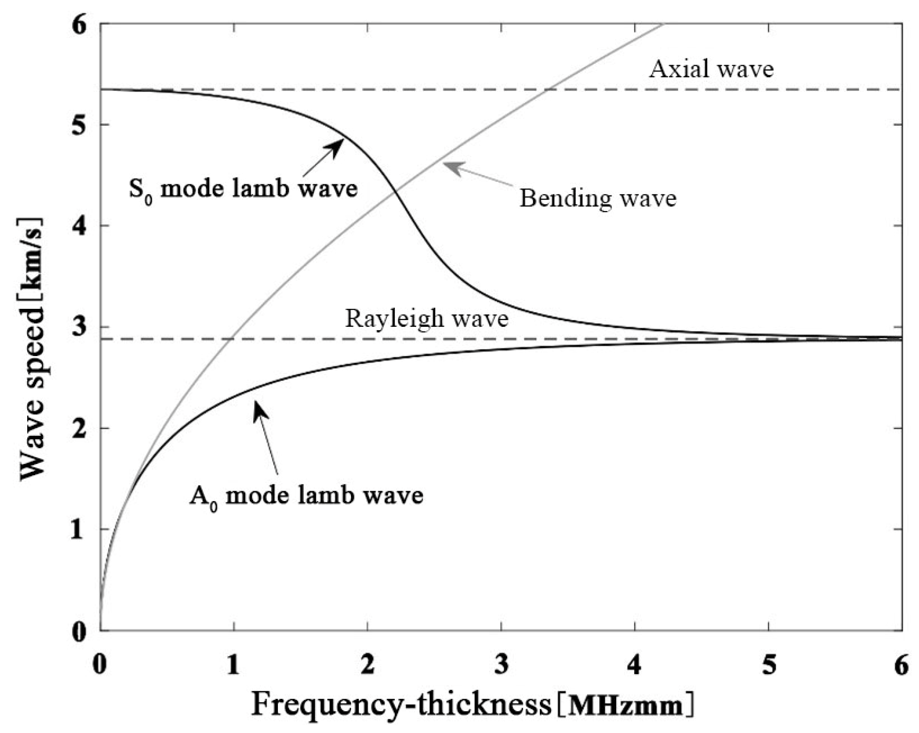
Apart from the fundamental symmetric mode of the shear horizontal wave, all other wave modes exhibit dispersive properties, meaning that the group velocity depends on the frequency of the propagating wave. In shear horizontal waves, the fundamental symmetric mode can be found at all frequencies, and each mode has a critical frequency at which it appears concurrently with the preceding mode. On the other hand, in Lamb waves, and for low-frequency thickness coefficients , two basic modes and can be observed. As this coefficient increases, other modes begin to appear and propagate simultaneously, depending on the dispersion curve of the material being processed. When , as the thickness is greater than one wavelength, symmetric and antisymmetric modes degenerate into Rayleigh waves, as shown in Figure 1. Conversely, when , mode disappears into an axial or longitudinal wave, and mode disappears into a plate bending wave. The appeal of low-frequency research lies in the lower dispersion of the fundamental modes and the reduced complexity of the problem due to the ability to excite specific modes and , making it attractive for study.

Figure 1.
In a 1 mm thick aluminum plate, the wave speed–frequency dependency relationships of axial waves, bending waves, Lamb waves, and Rayleigh waves are considered.
2.2. Basic Equations of Lamb Waves
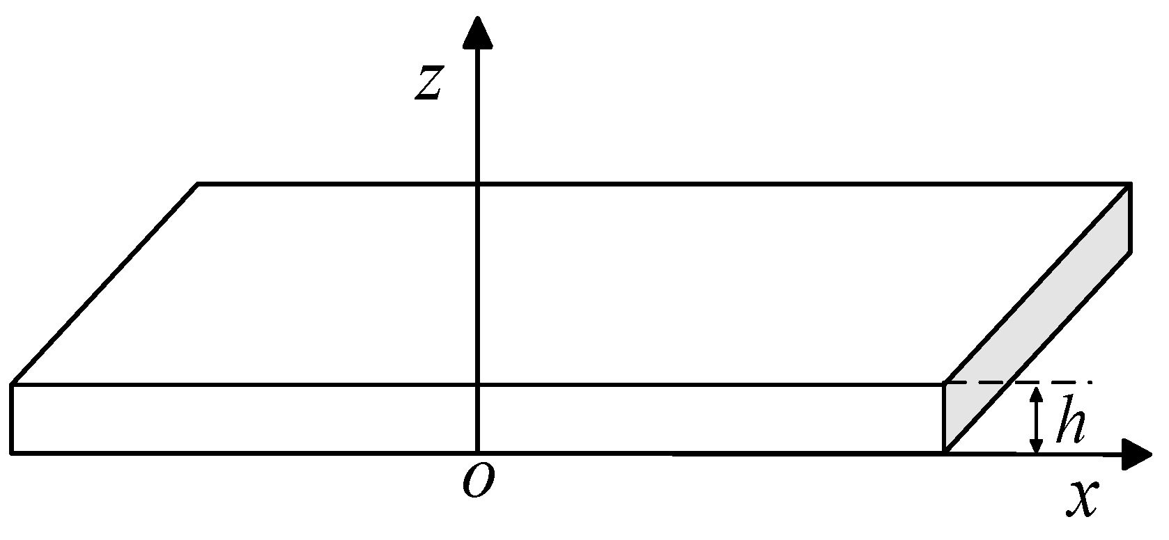
For the functionally graded material plate shown in Figure 2, the propagation direction of the Lamb plate is along the positive x-axis, and the z-axis is along the thickness direction of the plate, with a plate thickness of h. The material parameters vary continuously in the thickness direction, Where , the mass density and elastic coefficients , , are functions of the coordinate z.
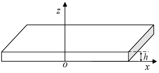
Figure 2.
Structural plate and coordinate system.
In this paper, the Lamb wave characteristics are described using the Rayleigh–Lamb wave equation [35]:
In the equation, , , represents the angular frequency, is the wave number where is the phase velocity of the plate. and are the longitudinal and transverse wave velocities, respectively, and is the thickness of the structure. Due to the nonlinear relationship between and , and are interconnected, leading to the occurrence of dispersion phenomena. This means that the propagation speed of different Lamb wave modes is correlated with their frequency. In practical scenarios, these modes propagate spatially with a group velocity .
2.3. Dispersion Curves of Lamb Waves
The dispersion curves of Lamb waves refer to the relationship between the longitudinal and transverse waves of Lamb waves in symmetric and antisymmetric modes as a function of frequency; that is, the wave speed–frequency curve. Since the wavelength and frequency of Lamb waves are influenced by factors such as the thickness of the structural plate and material properties, the dispersion curves of Lamb waves are closely related to the geometric dimensions and material parameters of the structural plate.
To obtain the dispersion curves of Lamb waves, it is necessary to construct the dispersion equations of Lamb waves. For a plate structure with an assumed thickness of 2 h, the Lamb dispersion curve equation is
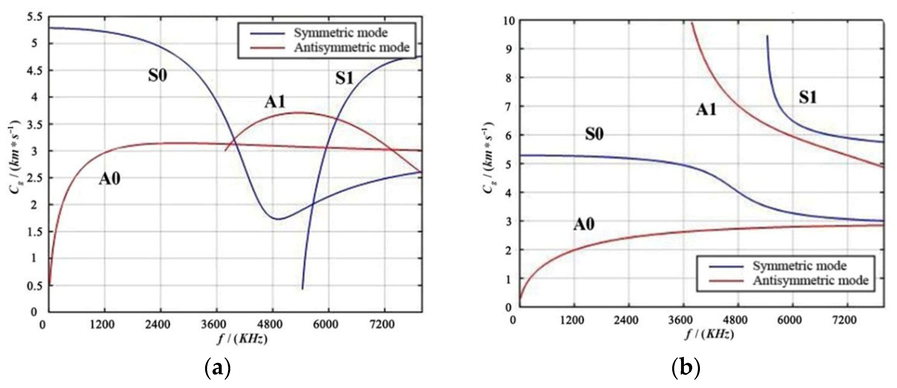
In the equation , represents the angular wave speed, represents the angular frequency, and represents the phase velocity of the material plate, while and are the longitudinal and transverse wave speeds of the plate, respectively. When the superscript in Equation (3) is +1, it represents the symmetric mode; when it is −1, it represents the antisymmetric mode. Solving the aforementioned Equation (3) yields the phase velocity dispersion curves and group velocity dispersion curves, as shown in Figure 3.
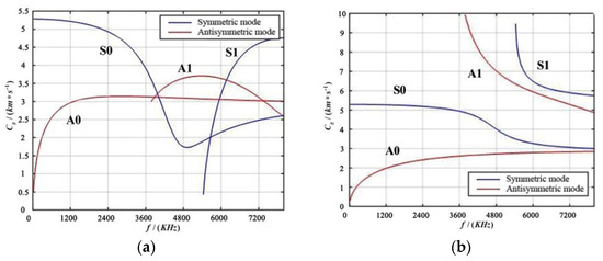
Figure 3.
Dispersion Curve Diagram of aluminum Plate. (a) Group Velocity Dispersion Diagram; (b) Phase Velocity Dispersion Diagram.
From Figure 3, it can be seen that in the group velocity dispersion curve, within the low-frequency range, there are and modes, and at 3600 kHz, and modes begin to appear; in the phase velocity dispersion curve, and modes appear at low frequencies, and at 3600 kHz, and modes appear. This indicates that for a three-dimensional aluminum plate, only waves of and exist at lower frequencies, while at higher frequencies, different modes of guided waves will appear, leading to mutual interference. In practical applications of structural damage monitoring, to reduce the dispersion and multimode effects of guided waves and simplify signal processing, Lamb waves of a single mode are usually selectively excited in the low-frequency range.
Typically, the mode is chosen as it helps alleviate the impact of wave dispersion and multimode characteristics. This selection facilitates easier signal analysis and processing.
For different modes of Lamb waves, the relationship between phase velocity and group velocity also varies. In the low-frequency range, the phase and group velocities and are relatively close so they can be used simultaneously for SHM. However, as the frequency increases, the difference between the phase and group velocities of higher-order modes becomes more pronounced, so the appropriate mode must be selected for monitoring and analysis according to the actual situation.
2.4. Physical Module and Control Equations of Finite Element Simulation
The simulation model of Lamb waves in this paper is developed in the transient acoustic pressure module of the COMSOL Multiphysics® version 6.2 software, which is based on the finite element method. This module is used to solve the control partial differential equations (PDE) for the propagation of sound waves as follows:
In the equation, represents the pressure of the sound wave (), represents the density of the material (), c represents the speed of the sound wave in the given medium (), represents the energy dipole domain source (), and represents the energy monopole point source ().
The fundamental concept behind implementing damage identification using Lamb waves involves leveraging the propagation characteristics of Lamb waves within a structure. By employing sensors to receive response signals, distinctive features related to damages are extracted from the received signals. These features are then employed to determine the structural damage state, identifying structural defects. When Lamb waves propagate to regions with defects or damages within the structure, alterations occur in their propagation characteristics, such as changes in wave velocity and amplitude. Consequently, by analyzing the received wave signals, it becomes possible to identify defects or damages.
However, due to the coexistence of multimodal behavior and dispersion characteristics in Lamb waves, Lamb wave signals are inherently intricate. This complexity presents challenges in signal analysis and processing, making it necessary to apply signal processing techniques and algorithmic refinement to extract damage-related features from the signals.
3. Theoretical Foundations
3.1. Fundamentals of the RPCA Algorithm
Robust Principal Component Analysis (RPCA) is an algorithm capable of extracting principal components from data containing outliers. Unlike traditional Principal Component Analysis (PCA), RPCA separates outliers and noise from the data while preserving the component information. The fundamental concept of RPCA involves decomposing the original data matrix into the sum of a low-rank matrix and a sparse matrix .
where contains the principal component information of the original data and contains the outliers and noise in the data.
Candès et al. [23] initially formulated the optimization model of the RPCA algorithm as follows:
represents the rank of the matrix , and denotes the number of nonzero in the matrix and also the sparsity of the matrix .
Since the norm problem has been proven to be an NP-hard problem, there is currently no direct optimal solution algorithm available. As a result, this problem has been relaxed into the following form:
where is the regularization parameter used to control the impact of the low-rank and sparse components on the objective function. represents the nuclear norm, which approximates the size of the matrix rank using a norm involving the singular values of the matrix. Computing the nuclear norm involves adding the absolute values of the singular values obtained after performing singular value decomposition. If the singular value vector is denoted as , then . represents the -norm of , which is defined as .
3.2. Augmented Lagrange Multiplier Method and Inexact Augmented Lagrange Multiplier Method
The Augmented Lagrange Multiplier Method (ALM) [36,37] is primarily used to solve problems with equality constraints. The general form is as follows:
In the above, and are the free variables; represents the objective term; denotes the equality constraint conditions. The optimization problem aims to adjust the magnitudes of and while satisfying the constraint conditions in order to minimize the objective term’s function value.
By introducing the dual variable , the aforementioned optimization problem with equality constraints is transformed into an unconstrained optimization problem. The augmented Lagrange function is constructed as follows:
where is the penalty coefficient. The general approach used to solve the above equation is by employing the dual ascent method. The ALM algorithm primarily aims to find the optimal solutions for two problems:
The method is mainly divided into two steps. In the first step, is held constant while solving for . In the second step, the gradient ascent method is utilized, and the solutions obtained for and are substituted into Equation (21). The parameter is used as the step size to update .
Due to the fact that the convergence of the ALM algorithm cannot meet the real-time requirements of practical problems, the IALM was proposed based on ALM. IALM is a distributed optimization algorithm [38] that exhibits a faster convergence rate than ALM. The solving process of IALM follows the same steps as ALM. Firstly, the augmented Lagrange function is constructed:
Then, the method employs an alternating computation approach to update and .
Compared to the ALM algorithm, which updates as a whole, IALM treats and as independent entities and alternately updates them. This approach effectively reduces computational complexity. Through this alternating update process of the two matrices, IALM employs element-wise thresholding operations to maintain non-negativity, gradually approaching an approximate solution to the original matrix. Therefore, for large-scale problems, IALM offers advantages such as fast convergence and good numerical stability.
4. The Non-Convex Approximate RPCA Algorithm
4.1. The Non-Convex Approximation of Rank
Although RPCA exhibits high robustness, it also has limitations. Firstly, the assumption of a convex nature for the low-rank matrix in RPCA does not hold true in certain cases, which affects the accuracy of the algorithm. Secondly, RPCA involves solving convex optimization problems to determine the low-rank and sparse matrices, and the slow convergence of convex optimization affects the efficiency of RPCA when dealing with large-scale problems. To address these issues, an improvement has been made by introducing non-convex functions to approximate the matrix rank and -norm. This enhancement modifies the low-rank and sparse matrices in RPCA and optimizes the solution of convex optimization problems to enhance computational efficiency.
The optimization model of RPCA is relaxed to
where , represents the ith singular value of the matrix .
Although Equation (16) is a convex problem and easily optimized, in practical scenarios, due to possible data corruption, obtaining the global optimal solution of Equation (16) may lead to significant errors. Furthermore, since the nuclear norm is essentially equivalent to the -norm of the vector of matrix singular values, the -norm exhibits a shrinkage effect that results in biased estimates. This implies that the nuclear norm excessively penalizes large singular values, causing solutions that deviate significantly from the true solution.
Therefore, a new non-convex approximation function is employed to approximate the rank of , which provides a closer approximation than the nuclear norm. The mathematical form of the non-convex function is defined as follows:
where represents the model parameter, represents the ith singular value of matrix .
The non-convex rank-approximation function y possesses the following characteristics:
- (1)
- ;
- (2)
- , ;
- (3)
- is unitary invariant, meaning that for any orthogonal matrix and , it holds that ;
- (4)
- For any matrix , it holds that , if and only if , .
Figure 4 illustrates the case of using the non-convex function and nuclear norm to approximate the rank function, with the value of increasing gradually. It can be observed that as the singular value increases, the nuclear norm deviates significantly from 1, while the non-convex function steadily approaches one more stably. A smaller parameter value leads to a better approximation of the rank function.
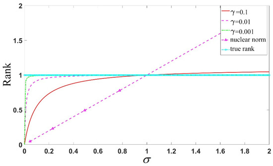
Figure 4.
Comparison of the approximation effects on matrix rank using different values for the approximation function and nuclear norm.
4.2. The Non-Convex Penalty Function
However, for the sparse component , G. Gasso et al. [39] demonstrated that adopting non-convex penalty functions can better approximate the sparsity properties of sparse signals and, under certain conditions, ensure the uniqueness of sparse solutions. Hence, a non-convex penalty function is utilized to approximate the sparse matrix S , denoted as the sparse penalty function . Suppose that the function is concave on (0, ∞), continuous, and monotonically increasing, and concave on (−∞, 0), continuous, and monotonically decreasing. Table 1 presents the non-convex penalty functions for approximating the sparse matrix , including the penalty function () [40], the logarithmic penalty function (), the exponential penalty () [41], and the Smoothly Clipped Absolute Deviation (SCAD) [42]. Table 1 lists these penalty functions along with their super-gradients., where represents the element at the ith row and jth column of matrix .

Table 1.
Non-convex penalty functions and their super-gradients.
All of Figure 5 exhibits the characteristic of sparsity, i.e., large gradients in some regions and small or zero gradients in others. Thus, to some extent, it is relevant to sparse learning. This is because, in sparse learning, the model is usually expected to have large gradients in certain parameters, which results in larger weights corresponding to these parameters and smaller or zero gradients in other parameters, thus achieving sparsity in the model.
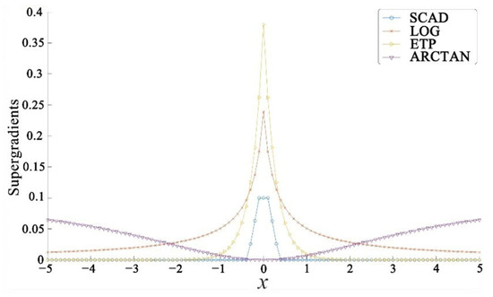
Figure 5.
Super-gradients function.
4.3. Derivation of the Overall Formula for NCA-RPCA Algorithm
From Section 4.1 and Section 4.2, the optimization problem can be redefined as follows:
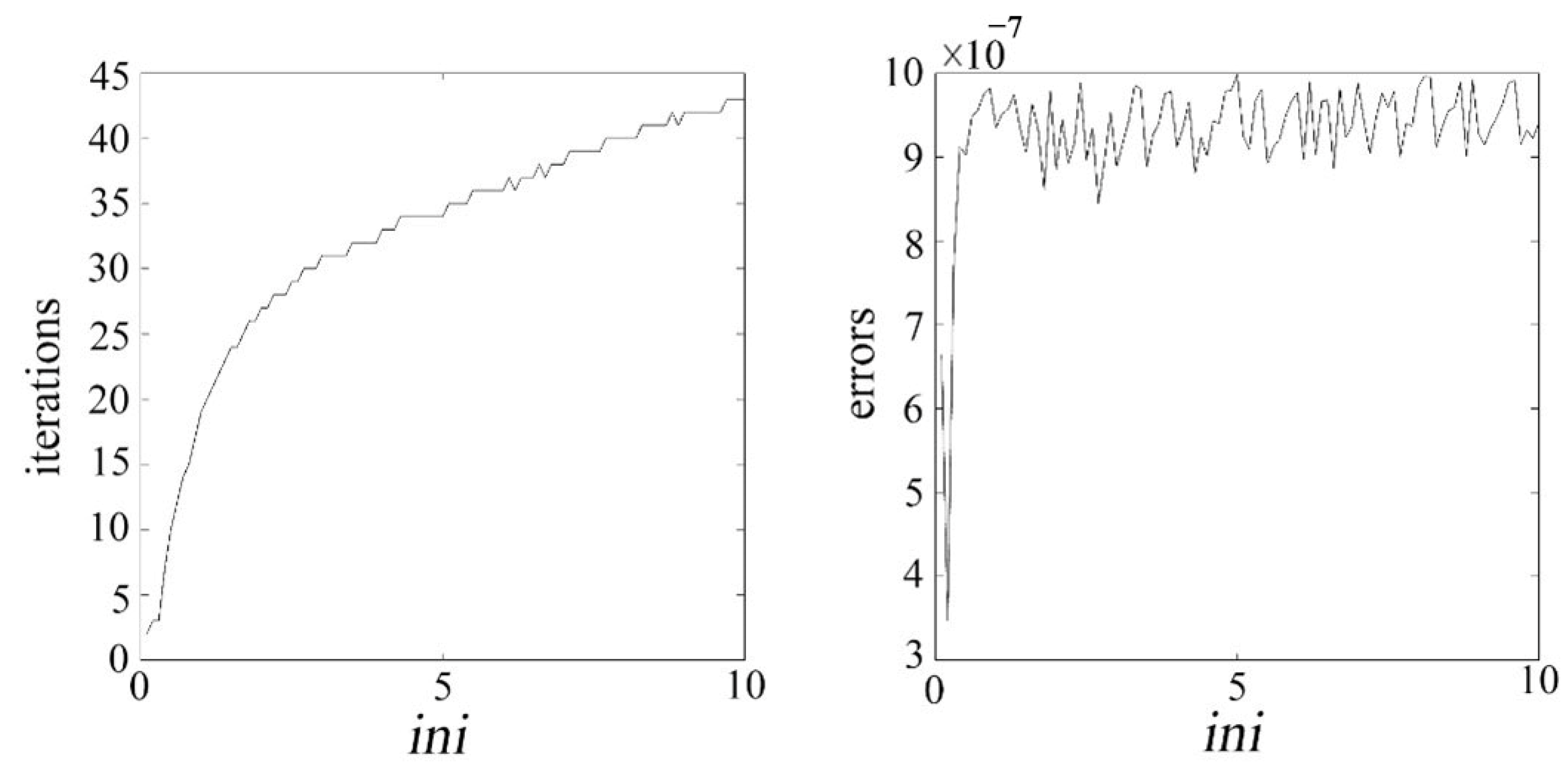
where represents the element in the ith row and jth column of matrix , the parameter determines the relative impact of low-rank and sparsity on the objective function. The optimal value of that balances the minimization of the rank of and the maximization of the sparsity of can be achieved by controlling . To determine the parameter , numerical experiments were conducted in this study, using the number of iterations and error value (err) as criteria for selection. Let , where is set within the range , and m and n are the rows and columns of the input image matrix, respectively. Figure 6 shows the relationship between the number of iterations, error value (err), and .
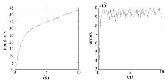
Figure 6.
Illustrates the relationship curve between the number of iterations, error value, and .
From Figure 6, it can be observed that as increases, the number of iterations continuously rises, and the error value also increases to some extent. Therefore, based on Figure 5, this study chooses to determine the value of parameter . The role of is to balance the low-rank and sparse components of the matrix, while affects the threshold of the non-convex penalty function. Thus, these two parameters need to be jointly adjusted to achieve a balance between the low-rank and sparse components. The penalty coefficient , following the approach in reference [30], is set as . This process ultimately leads to a well-optimized set of parameters for the algorithm.
When seeking a solution for Equation (18), the properties of the function can be derived from the gradient (or super-gradient when there is a non-smooth origin point). At the point , if holds for every ; then, is the super-gradient of function . Thus, the function in Equations (17) and (18) has its approximated formulation as , where is sufficiently close to . By using first-order Taylor expansion, represents the gradient of at . The same principle can also be implemented for the penalty function .
Expanding and using the first-order Taylor series, the Lagrangian form of the optimization problem described above can be established based on Equation (9).
where the dual variable is the Lagrange multiplier and is the penalty coefficient. For the sake of convenience in subsequent calculations and processing, and can be combined.
Here, can be treated as a constant when solving for and , thus Equation (20) can be scaled. In other words, can be equivalently represented as .
Continuing, the IALM is employed to solve the equation, mainly involving three steps: in the first step, and are fixed, and is updated to find its optimal value. Since is independent of , it can be omitted during the process of solving for . is a constant, and it can also be omitted and scaled while solving for , as follows:
Because in Equation (32), represents the first-order Taylor expansion of and is a constant; therefore, during the process of solving for , can be omitted, meaning that is equivalent to . The above equations are derived and simplified.
In the second step, with fixed along with the updated , the optimization of is performed to obtain the optimal value of . Similarly, it can be observed that is independent of during the process of solving for , and thus can be omitted.
Due to the first-order Taylor expansion of being equivalent to and being a constant in Equation (26), during the process of solving for , it is possible to omit , meaning that is effectively equivalent to . The above equations are derived and simplified.
In the third step, with the updated and fixed, the gradient ascent method is applied to update , updating the penalty parameter using the step size .
where denotes the iteration number. The specific solving process is as follows:
Step one, fixing and , update :
Let and decompose the above equation into a subproblem regarding , then the equation becomes:
where and are elements of and , respectively. For the sake of simplicity in notation, the subscripts i and j are omitted. Regarding the equation, the soft-thresholding operator [43] can be applied to solve for , which can be obtained from the following equation:
Here, represents .
Second step, with and fixed, update :
Let , then the above equation becomes
Performing the singular value decomposition on , we have , where the diagonal matrix of singular values is represented by . The jth singular value of is denoted as , and the jth singular value of is
According to the singular value soft-thresholding operator [43], the optimal solution for is given by
Therefore,
where is the column vector composed of , and and are matrices obtained from the singular value decomposition of .
Finally, update the Lagrange multiplier and the penalty parameter .
If the convergence condition is satisfied in the iteration, meaning that the difference between the observed matrix and the reconstruction of the low-rank and sparse matrices is smaller than a given threshold, then at this point, and are very close to the actual low-rank and sparse components. It can be considered that the decomposition results are relatively stable. Therefore, output and , and the entire algorithm process concludes.
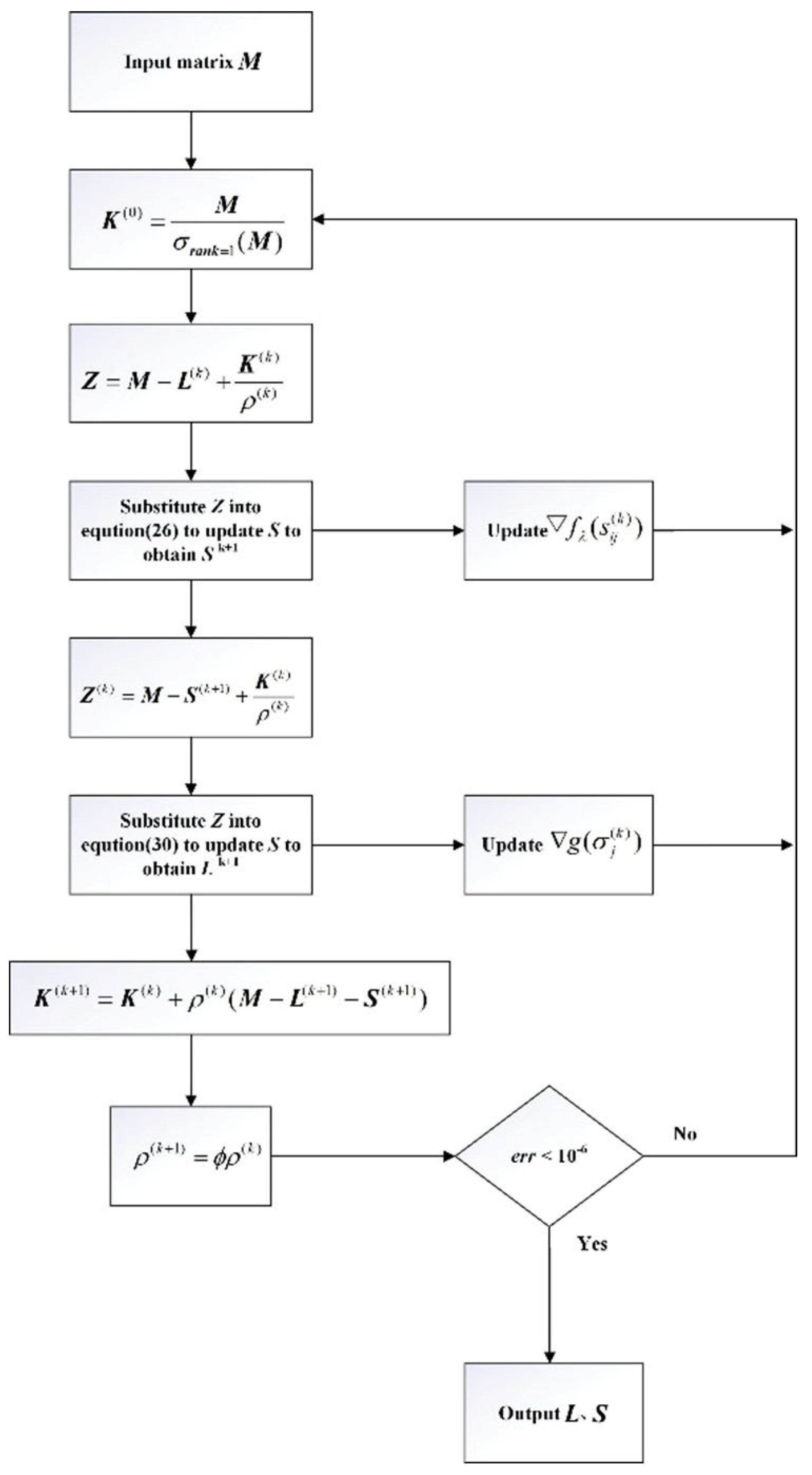
Based on the algorithm procedure described above, create a flowchart. Assuming the input original data matrix is and the outputs and are the low-rank and sparse components of , the flowchart of the NCA-RPCA algorithm is illustrated in Figure 7.
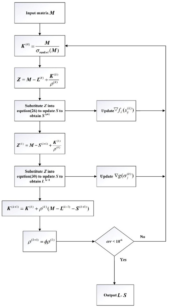
Figure 7.
NCA-RPCA algorithm flowchart.
5. Damage Detection in Wavefield Images Based on NCA-RPCA Algorithm
5.1. Establishment of Lamb Wave Damage Model and Parameter Selection
5.1.1. Model Establishment
In this paper, a 3D plate model is used; the material chosen is aluminum, and the direction of study is transient. The structure of the 3D aluminum plate is shown in Figure 8. Firstly, a square with a side length of 200 mm is constructed, and another square with a side length of 180 mm is constructed in the square, and then these two squares are overlapped, and the overlapped area is set as a damping layer, which can simulate the energy dissipation mechanism existed in the structure, to more realistically reflect the propagation state of the Lamb wave in the actual situation; and the boundary is set as a low-reflection boundary; next, the combination is stretched by 1 mm and the edges are set as stick supports, which can ensure that the boundary will not shake in the process of Lamb propagation. The specific parameters of the 3D aluminum plate material are shown in Table 2.
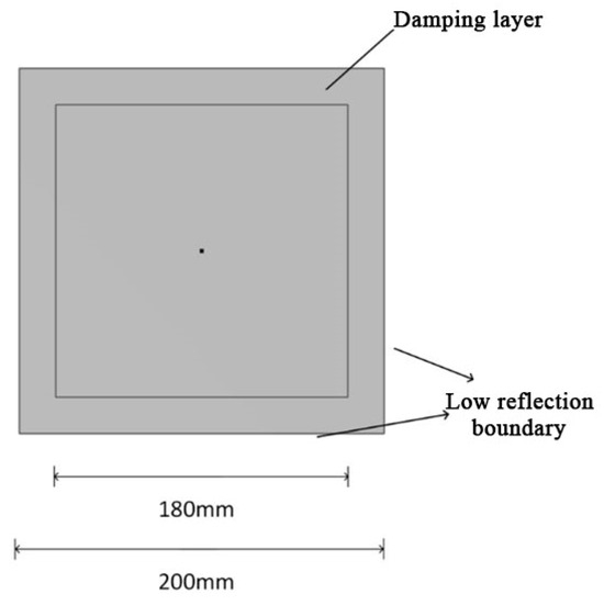
Figure 8.
Three-Dimensional aluminum plate structure.
Table 2.
Structural material parameters.
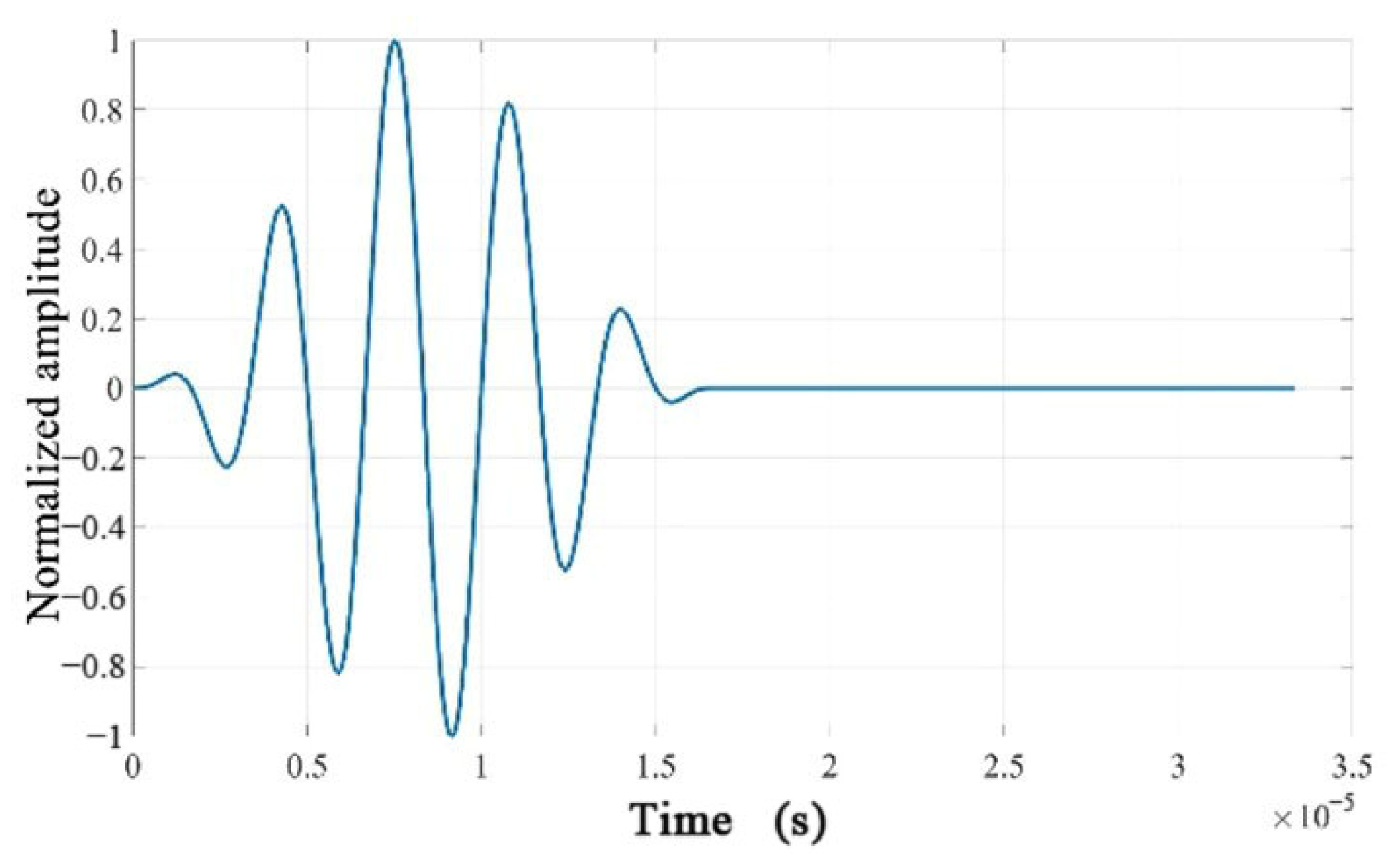
During the COMSOL finite element simulation experiments, to excite and propagate Lamb waves within the plate structure for obtaining a dataset, it is necessary to establish an excitation. The expression for the excitation signal is as follows.
where, is the center frequency of the Hanning window, and is the number of wave cycles. This study confides the excitation as a sine wave modulated with a Hanning window containing five cycles.
The center frequency is generally preferred to be set between 150 kHz and 500 kHz. If the excitation signal’s center frequency is set too low, it may not excite the desired modes, especially the mode, as the mode corresponds to relatively higher frequencies. Low-frequency excitation might result in significant energy loss, preventing effective propagation and focusing of the wavefield energy. On the other hand, setting the excitation frequency too high can excite more complex modes, causing greater interference in the signal. High-frequency signals also correspond to very short wavelengths, potentially leading to simulation results that do not align with physical reality. In this study, to compare different frequencies, as shown in Figure 9, the selected center frequency is 300 kHz. This selection aims to control the excitation’s duration and concentrate the signal, reducing harmonic generation. It also enhances the visibility of the wave packet associated with the mode, which is essential for structural damage detection. The excitation signal is shown in Figure 10.

Figure 9.
= 100 kHz (left); = 300 kHz (middle); = 600 kHz (right).
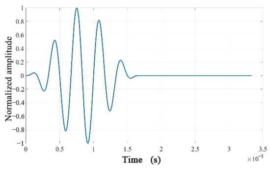
Figure 10.
Time-domain waveform of the excitation signal.
5.1.2. Simulation Parameter Configuration
Since the focus of this experiment is on transient analysis, it is necessary to set a reasonable time increment to ensure the stability and convergence of the transient analysis. If the time increment is too small, it will increase computation time and cost. On the other hand, if the time increment is too large, it may lead to numerical instability and reduced accuracy. The time increment for the finite element model needs to satisfy the Newmark time integration scheme [44], which is given by
Since the selected is 300 , which corresponds to , in order to achieve a higher temporal resolution, the actual simulation calculations use .
Similarly, the grid size plays a crucial role in the stability and convergence of finite element analysis simulations. The relationship between the grid size and the wavelength of Lamb waves needs to satisfy the following condition [45].
where represents the minimum wavelength of Lamb waves under the selected excitation. This minimum wavelength typically corresponds to the highest-frequency mode of Lamb waves, which is the shortest periodic vibration mode within the structure. Larger grid sizes lead to increased errors in accuracy, as shown in Figure 11. When the grid size , it can result in distorted wave characteristics, causing deformation or distortion in the waveform. This misestimation of the waveform shape and amplitude leads to inaccurate estimation of the propagation path of Lamb waves, consequently affecting the accuracy of simulation results and compromising their validity. Therefore, while ensuring result accuracy, reducing the grid size is crucial to decreasing computational load and enhancing computational efficiency. Hence, the minimum wavelength can be deduced as , leading to , with the actual selection being .

Figure 11.
Wavefield images of failed grids.
5.1.3. Algorithm Parameter Selection
In this experiment, a number of wave damage images with different positions, sizes, and numbers were selected for processing, and all the pictures were processed with a resolution of 768 × 768 and the consistent resolution of the pictures is beneficial to unify the processing flow and improve the processing efficiency, as well as facilitating the comparison and output of the results. In order to simulate the actual situation, noise was added to each picture again, and the effect of noise on the outliers was studied by increasing the experiments with different noise densities. In order to further analyze the relationship between outliers and noise, the adaptive thresholding method is used, and the noise is processed according to different threshold parameters “a”. By observing the changes in the number of outliers under different noise density conditions as the threshold “a” change, we hope to reveal the correlation between noise density and outliers, as well as the effectiveness of the adaptive thresholding method in dealing with noise, and the experimental results are shown in Figure 12. These experiments will help validate the effectiveness of our algorithm in complex noise environments and provide a more in-depth understanding and guidance for damage recognition in real scenes.
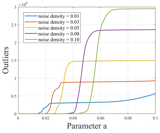
Figure 12.
Relationship curve between different noise densities and the threshold “a” for outliers.
From Figure 12, an evident trend can be observed: a clear positive correlation exists between noise density and the number of outliers. As the noise density increases, the number of outliers also increases, which is not favorable for subsequent data processing. Excessively low noise density may lead to an overly idealized scenario that does not align with real-world conditions. Thus, noise density is a crucial influencing factor that requires careful selection to ensure the accuracy and reliability of subsequent data processing. In this context, we opted for an intermediate value, selecting a noise density of 0.05 to provide a better simulation of real-world situations.
After determining an appropriate noise density, the impact of varying the threshold “a” on damage detection outcomes was also studied, particularly for images with different locations of damage. In scenarios with higher noise density, increasing the threshold “a” can effectively enhance noise removal. Conversely, setting “a” too low might overly retain noise, leading to outcomes that do not align with reality. Therefore, when selecting the value of “a”, it is necessary to strike a balance between noise reduction and information preservation.
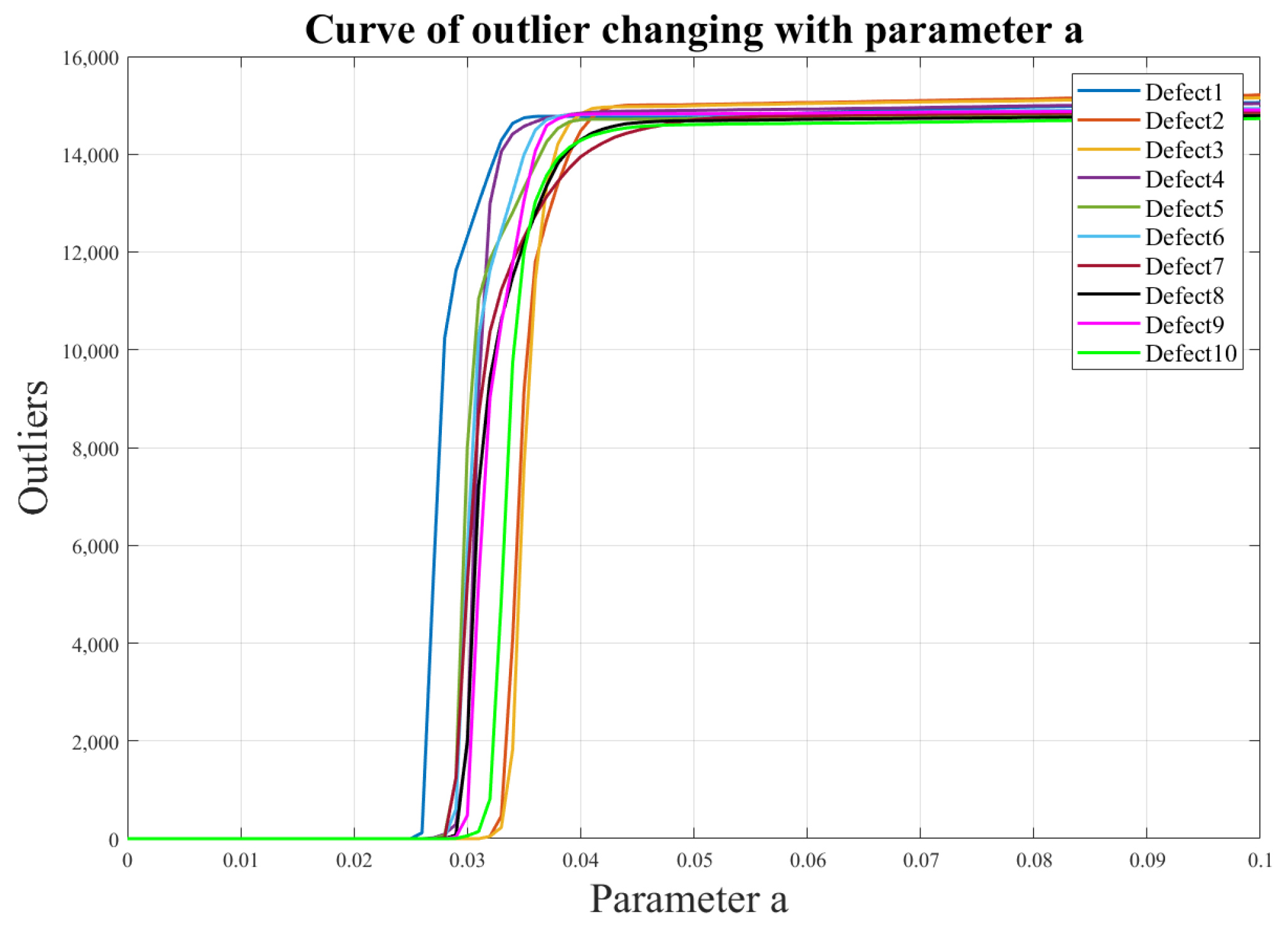
For the 200 mm × 200 mm aluminum plate, 10 defects were selected at different positions (varying both horizontal and vertical coordinates), and their threshold values were defined within a certain range. The results, shown in Figure 13 and Figure 14, reveal that these threshold values for different defect locations exhibit a relatively small and stable fluctuation range, ranging from 0.027 to 0.033. Consequently, by selecting a threshold value of 0.033, excellent identification outcomes can be achieved for various defect locations. This threshold value effectively filters out unwanted interferences while retaining the sparse values of interest, namely, the damaged regions. This finding is of significant importance for the excellent optimization of our algorithm.
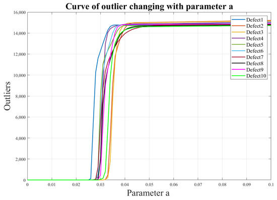
Figure 13.
Illustrates the curve depicting the variation of the number of outliers under different defects as the threshold “a” changes.
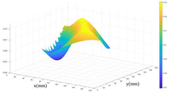
Figure 14.
The 3D plot of parameter selection for “a”.
5.2. Wavefield Image Damage Identification of Single Defects Based on NCA-RPCA Algorithm
5.2.1. Defects in Intermediate Positions
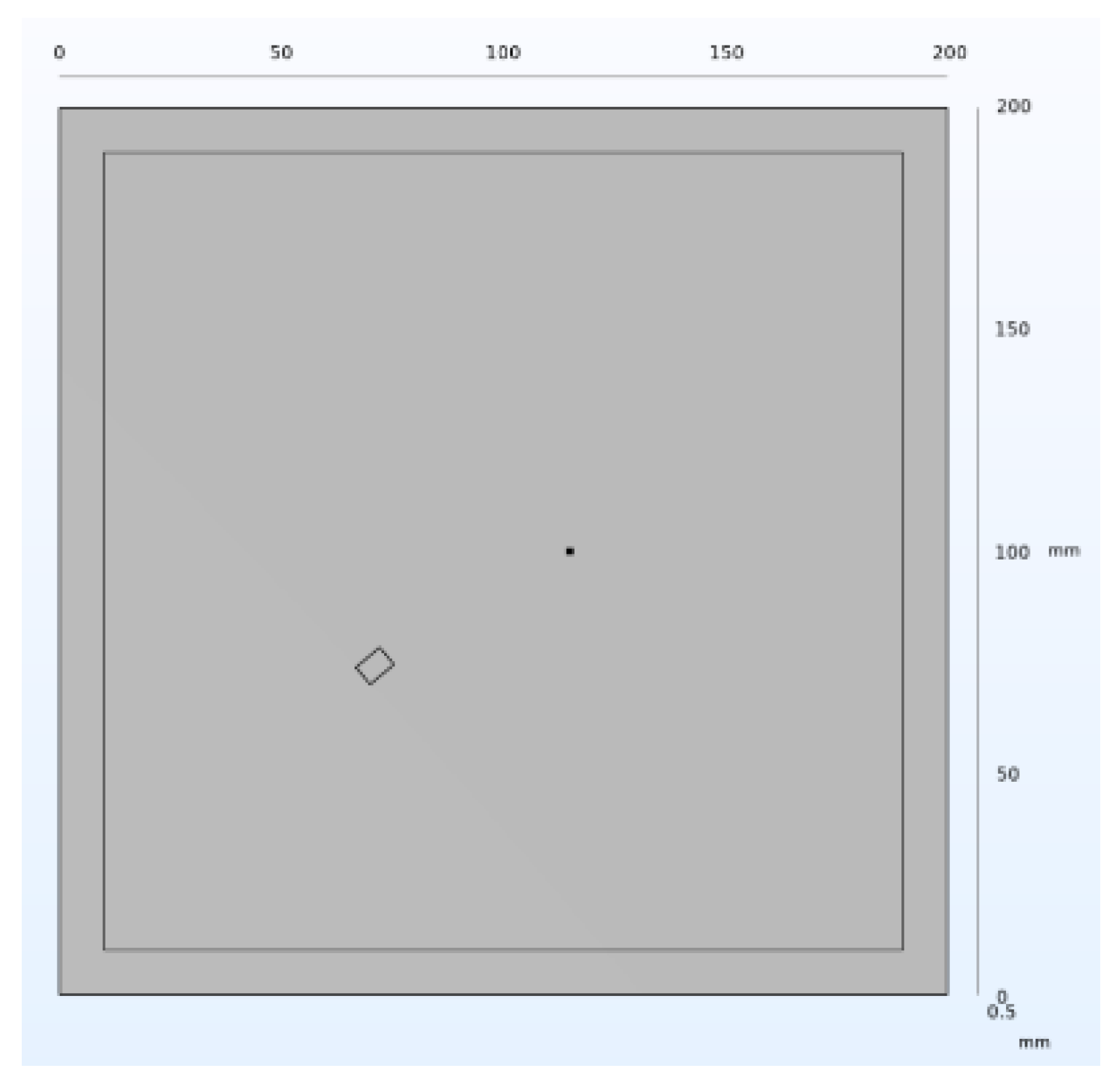
A rectangular central defect with dimensions of 5 mm width, 7 mm depth, and 0.5 mm height was introduced on the three-dimensional aluminum plate. This is illustrated in Figure 15.
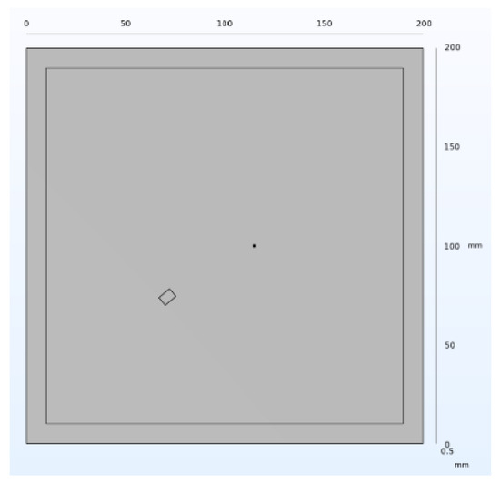
Figure 15.
Structure of the middle defect.
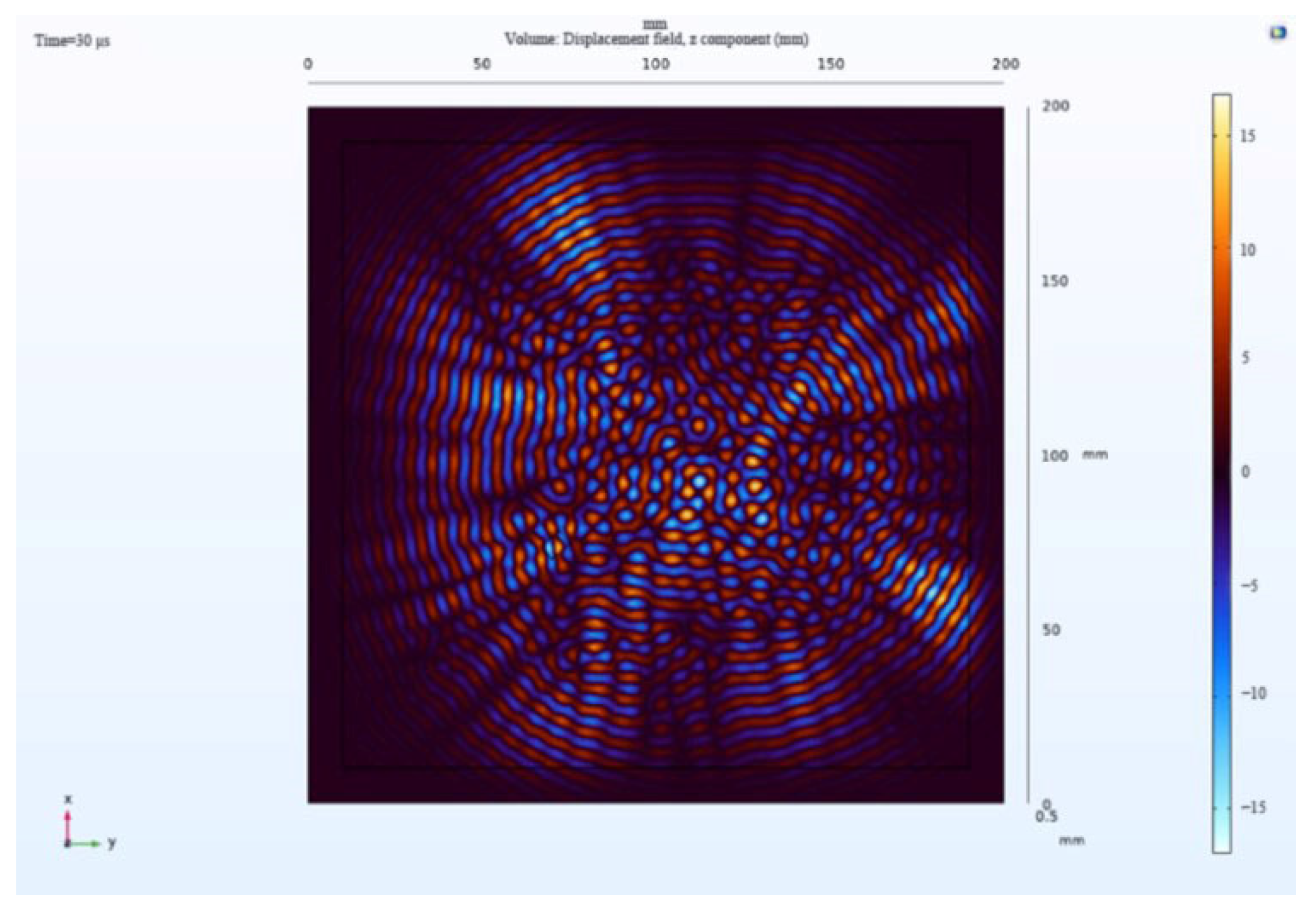
The receiving nodes deployed on the 3D aluminum plate can obtain the wavefield images at different output moments after the solution operation. Figure 16 shows that the Lamb wave completes its transmission at the defect location at 30 us, which visualizes the wavefield image of the Lamb wave that has been reflected and scattered after encountering the damage. It can be clearly seen that the Z-axis displacement component at the defect has changed. When the Lamb wave encounters a defect during propagation, it will change the propagation path of the wave and the upper and lower interface conditions, thus damaging the echo and scattering signals. The color table on the right side of Figure 16 can reflect the fluctuation of the Lamb wave in the process of propagation; the bigger the fluctuation, the closer the color is to the upper color, and vice versa, the closer the color is to the lower color, the modes of the Lamb wave will change accordingly, and the NCA-RPCA algorithm is very sensitive to the detection of the anomalous values. The algorithm processing can identify the damage more quickly and accurately; the results are shown in Figure 17, and the original image data matrix is decomposed into a low-rank matrix and a sparse matrix.
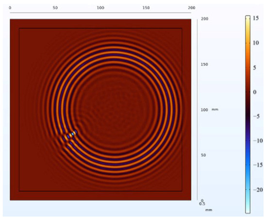
Figure 16.
Wavefield image of the middle defect.
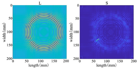
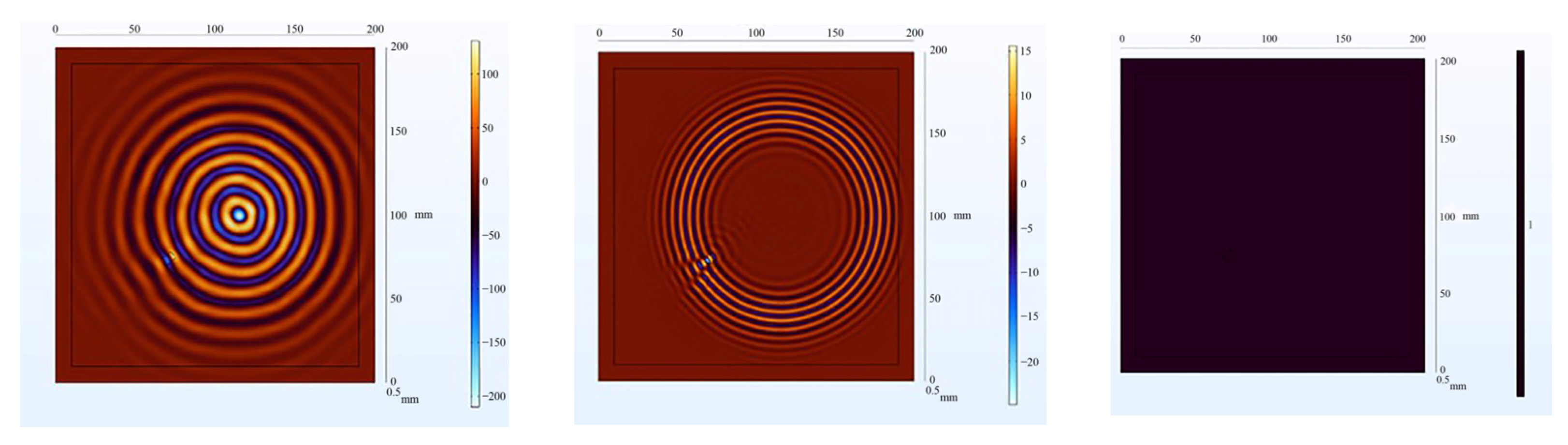
Figure 17.
The decomposition results of the NCA-RPCA algorithm.
After processing by NCA-RPCA, the principal information in the image data matrix is retained in the low-rank matrix, while the outliers are put into the sparse matrix. Since there are noise and outliers in the sparse matrix, it is also necessary to detect the defects corresponding to them by selecting a suitable threshold to remove the other noisy parts through the adaptive thresholding method. In this way, defects can be successfully detected regardless of their size, number, and location. The sparse matrix after denoising is shown in Figure 18, and then the damage can be identified in the original image by processing the nonzero ranks of the sparse matrix for identification, as shown in Figure 19.
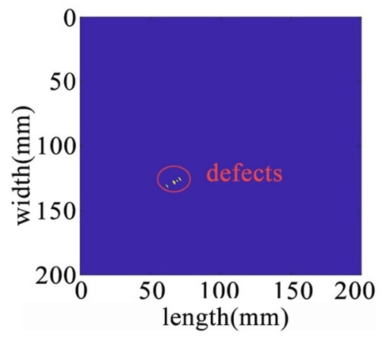
Figure 18.
The sparse matrix after denoising.
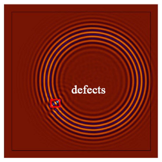
Figure 19.
Recognition results in the original image.
5.2.2. Defects at the Edge Positions
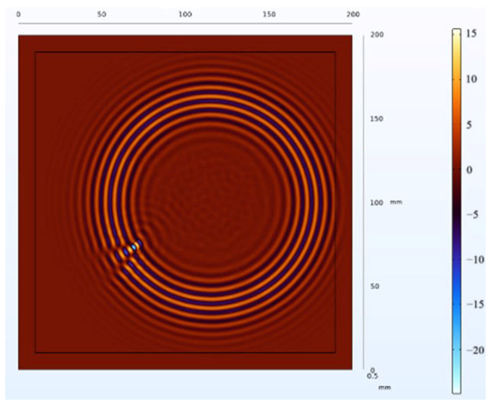
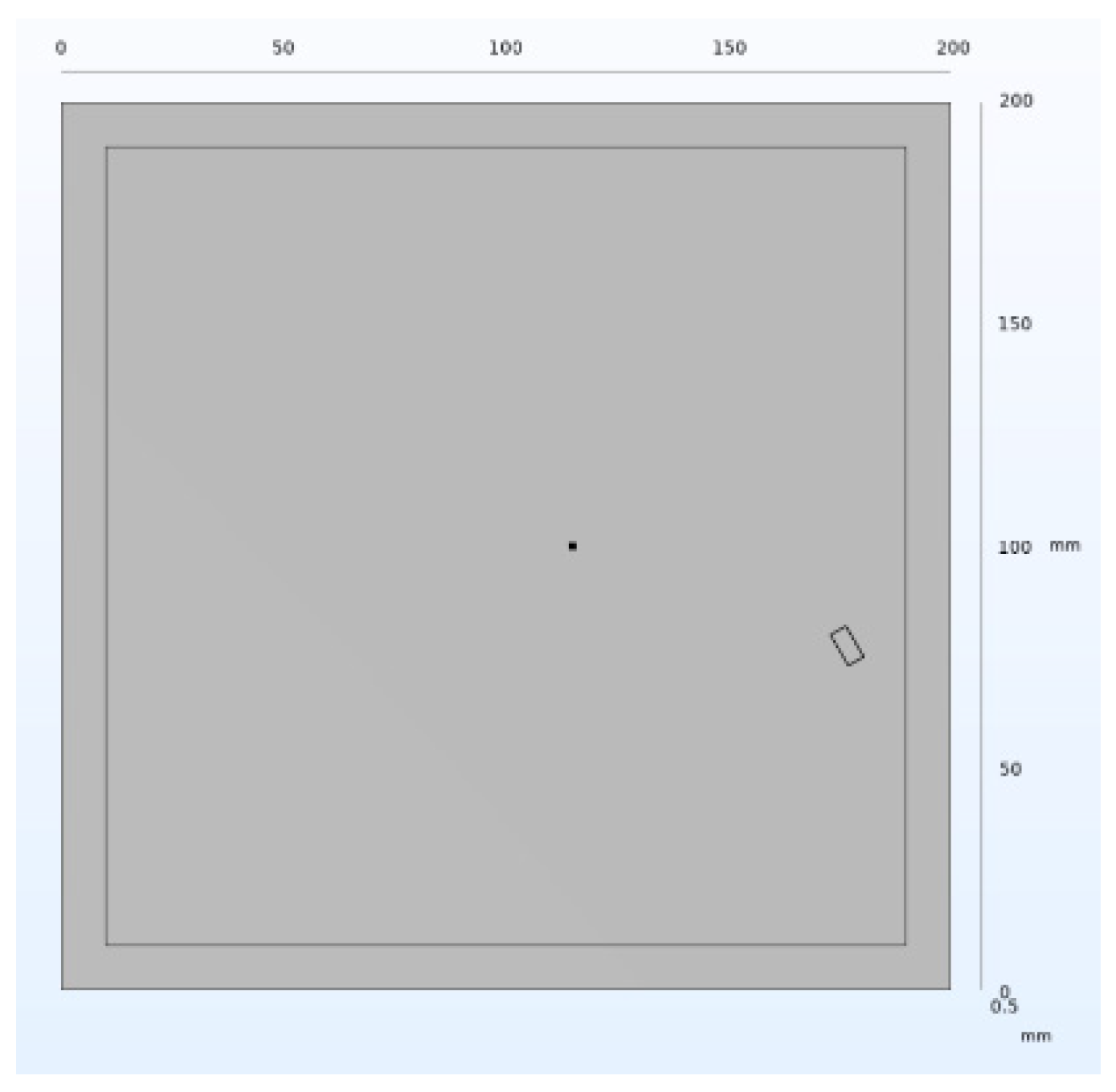
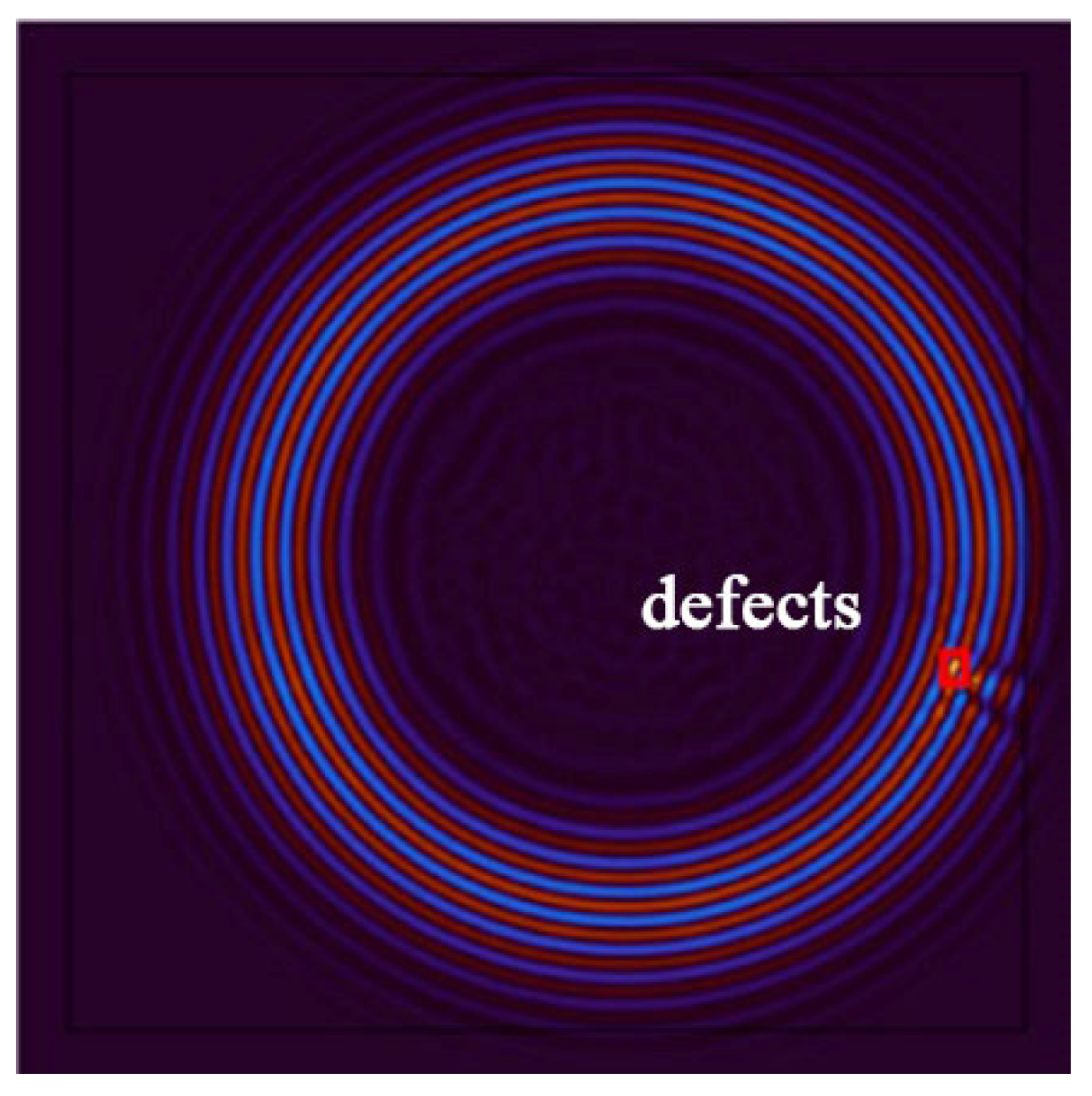
To closely simulate real-world scenarios, this study further investigates the identification results when defects are positioned at the edges of the plate. In the experiment, a new aluminum plate model was established, as illustrated in Figure 20. A rectangular edge defect with a width of 4 mm, depth of 8 mm, and height of 0.5 mm was placed on the aluminum plate, altering the defect’s location and size. After applying excitation, a time frame of 32 was selected for capturing the wavefield image, at which point the Lamb wave propagation at the location of the defect had concluded, as shown in Figure 21.
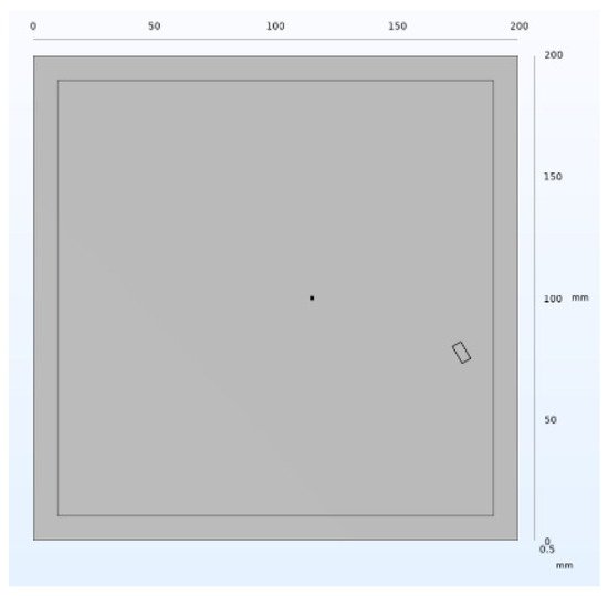
Figure 20.
Edge defect structure diagram.
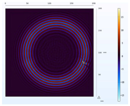
Figure 21.
Wavefield image of edge defect.
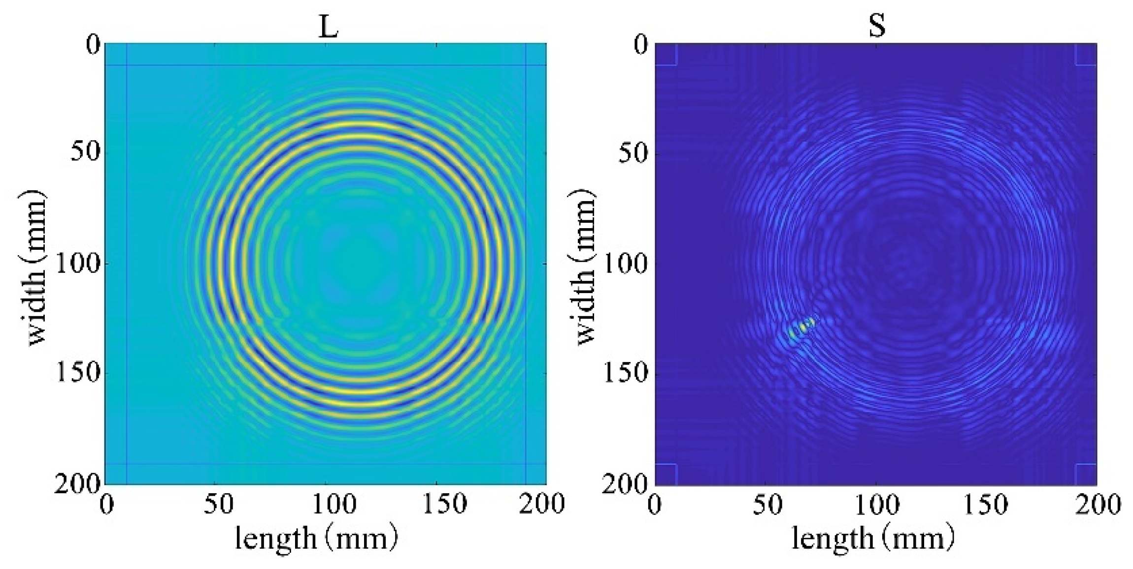
Due to the defect being located at the edge of the plate, the propagation time of Lamb waves is longer compared to the previous scenario. The reflections and scattering signals from the plate boundary introduce greater interference to anomaly detection. Applying NCA-RPCA to this image for defect detection, as seen in the decomposed result in Figure 22, still allows for a relatively clear identification of the sparse defect region. To achieve more accurate defect identification, an adaptive thresholding method is still needed to remove other noise sources, as depicted in Figure 23 and Figure 24.
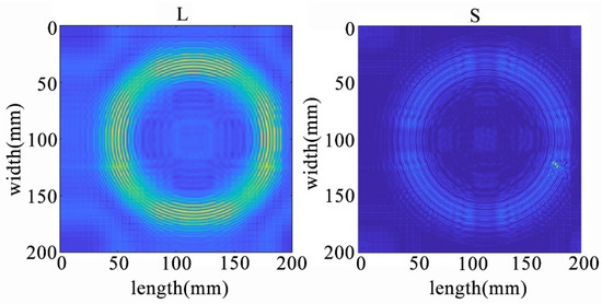
Figure 22.
The decomposition results of the NCA-RPCA algorithm at the edge of the plate.
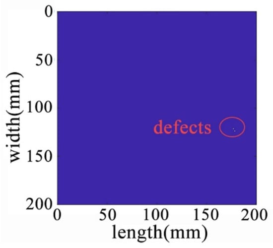
Figure 23.
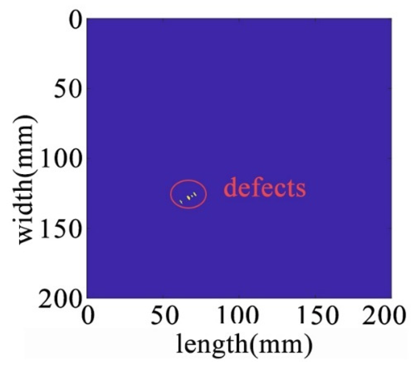
The sparse matrix after denoising at the edge of the plate.

Figure 24.
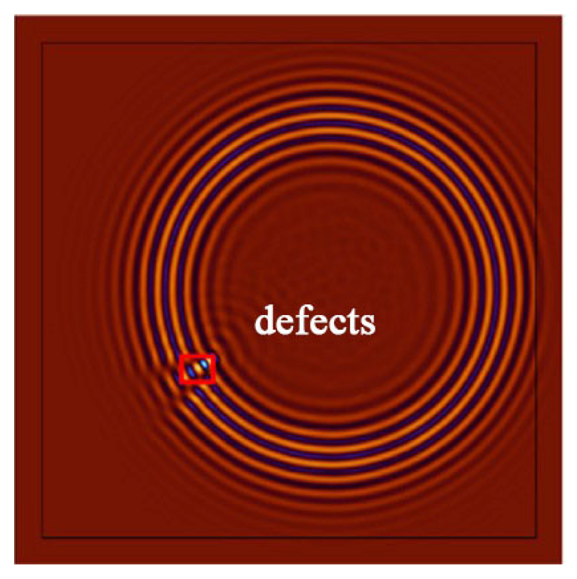
Recognition results in the original image at the edge of the plate.
When the defect is located at an edge position, due to the presence of more reflections and scattering signals around the edges of the plate, compared to defects in the central location, there will be more interference signals, significantly enhancing the difficulty of detection. Moreover, the size of the defect becomes smaller. However, the algorithm is still capable of accurately decomposing the original data image into effective low-rank and sparse abnormal value components. This allows for the rapid and accurate detection of defects within the image. This demonstrates that regardless of the defect’s size, shape, or position, the algorithm can effectively identify it, further confirming the validity and practicality of the approach.
5.2.3. Wavefield Image Damage Identification of Multiple Defects Based on NCA-RPCA Algorithm
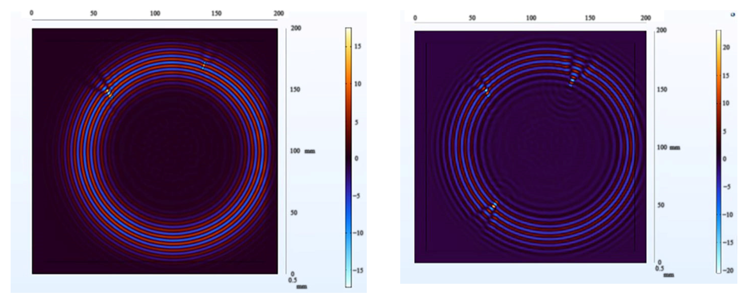
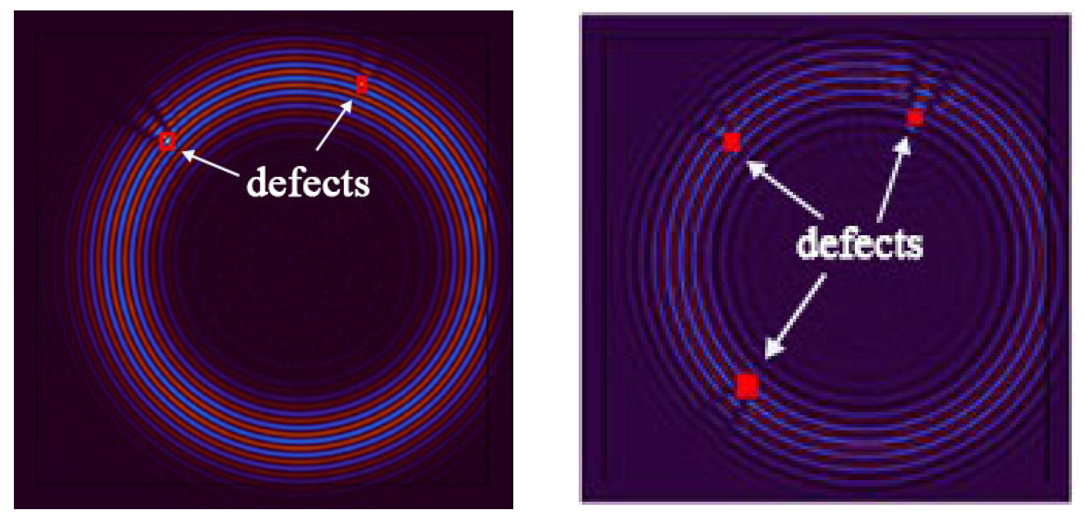
In the process of further demonstrating the effectiveness of the algorithm, we conducted another round of experiments using wavefield damage images. Initially, we changed the positions of the defects and increased their number. This implies that the algorithm needs to face more complex and diverse challenges. We increased the number of defects to two and three, respectively, with each defect having different shapes, sizes, and positions. Among them, one defect was made smaller. After constructing these scenarios, we applied the algorithm for defect detection, and the extracted wavefield damage images are shown in Figure 25.
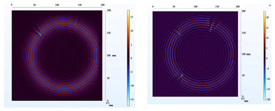
Figure 25.
Wavefield damage images for two different defects (left); three different defects (right).
Using the adaptive thresholding method to remove noise and irrelevant information, the results are shown in Figure 26 and Figure 27. After the denoising process, the algorithm successfully retained the targeted anomalies for identification. While effectively preserving the desired anomalies, the denoising process contributes to enhancing the algorithm’s excellence and stability. By reducing redundant information in the image, the computational complexity of the algorithm is reduced, leading to faster processing speeds. This, in turn, results in improved excellence, especially in real-time or large-scale data processing scenarios.
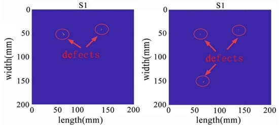
Figure 26.
The denoised sparse images with two defects (left) and three defects (right).

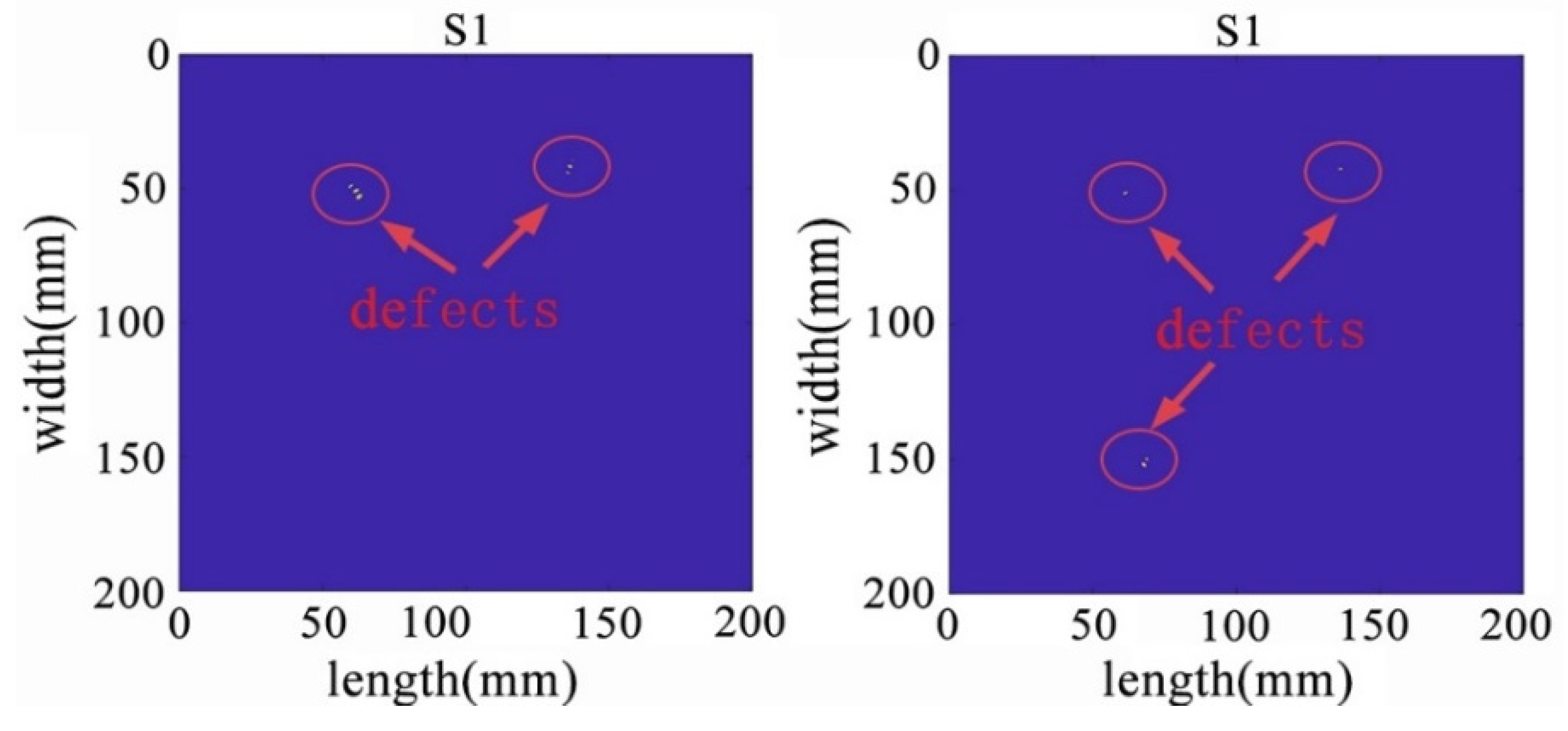
Figure 27.
The identification results of two defects (left) and three defects (right).
The algorithm successfully and accurately identified two distinct defects, one of which was particularly pronounced and featured finer details. This further underscores the remarkable excellence and adaptability of the algorithm in multi-defect detection scenarios. It demonstrates that the algorithm maintains a high detection capability for various types of defects, whether they are larger defects or subtle details, providing precise identification and localization. In real-world engineering scenarios, a variety of complex defects may arise, potentially with varying numbers and types. To evaluate the algorithm’s robustness and scalability, as well as its potential to handle multi-defect situations in practical engineering applications, the number of defects was further increased.
The results demonstrate that the NCA-RPCA algorithm not only performs exceptionally well in detecting single defects but also exhibits outstanding excellence when dealing with multiple defects. Whether facing single or multiple defects, the algorithm is capable of accurately identifying and reliably marking them. Detecting multiple defects is a complex and challenging task, as these defects might possess different shapes, sizes, and locations, and their proximity could introduce interference, increasing the complexity of detection. However, the algorithm showcases remarkable robustness and adaptability, successfully detecting all defects accurately. This further substantiates the algorithm’s reliability and effectiveness in various defect scenarios.
5.2.4. Comparison of Algorithms
To comprehensively demonstrate the superiority of the algorithms in this chapter, this paper conducts an in-depth comparative analysis with mainstream algorithms such as IALM, Accelerated Proximal Gradient (APG), RPCA-GD algorithm, and Fast Principal Component Pursuit (FPCP) algorithm. It will showcase the different handling effects achieved by combining various non-convex penalty functions with non-convex rank approximation functions, providing a multi-angle display of the advantages of the approximation methods proposed in this paper.
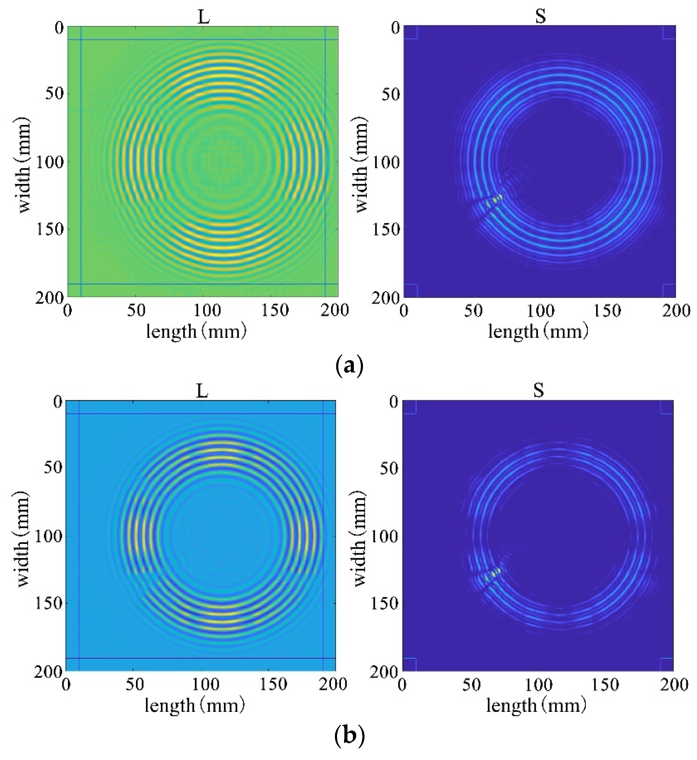
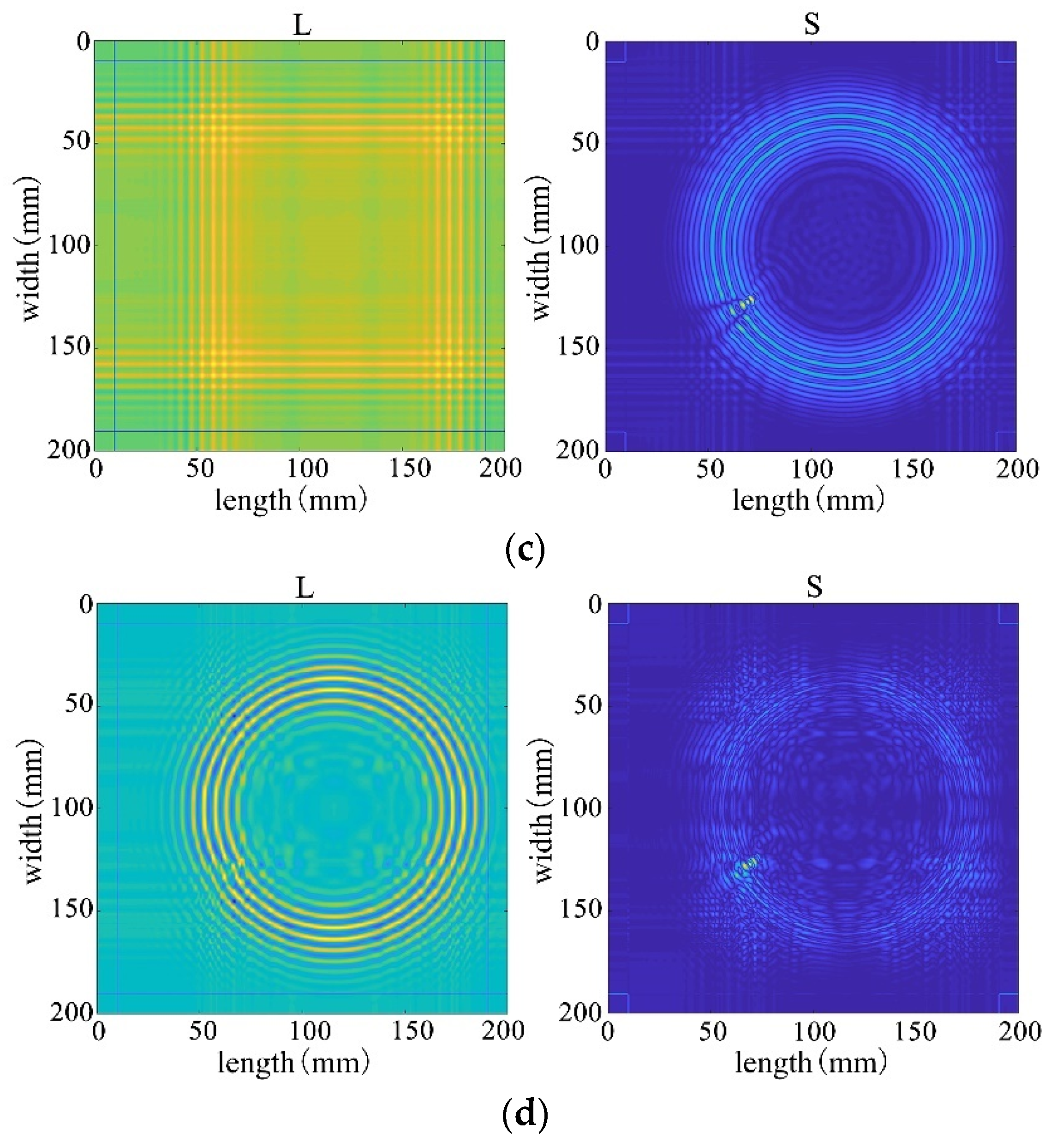
First, four mainstream algorithms were used for processing, and the results showed significant limitations when handling wavefield damage images. In Figure 28a,b, the IALM and APG algorithms decompose the sparse matrix, but they excessively categorize useful information as anomalies, resulting in severe information loss and unsatisfactory processing effects. In Figure 28c, the FPCP algorithm fails to effectively retain useful information or separate outliers after decomposition. The decomposition results in Figure 28d are relatively better.
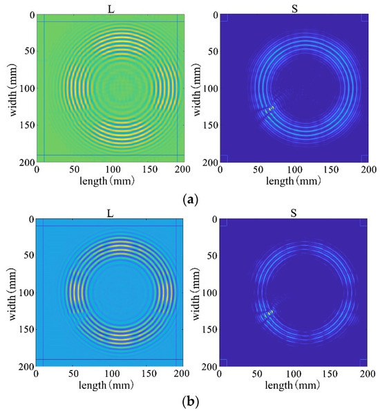

Figure 28.
Decomposition result of traditional algorithms. (a) IALM decomposition result. (b) APG decomposition result. (c) FPCP decomposition result. (d) RPCA-GD decomposition result.
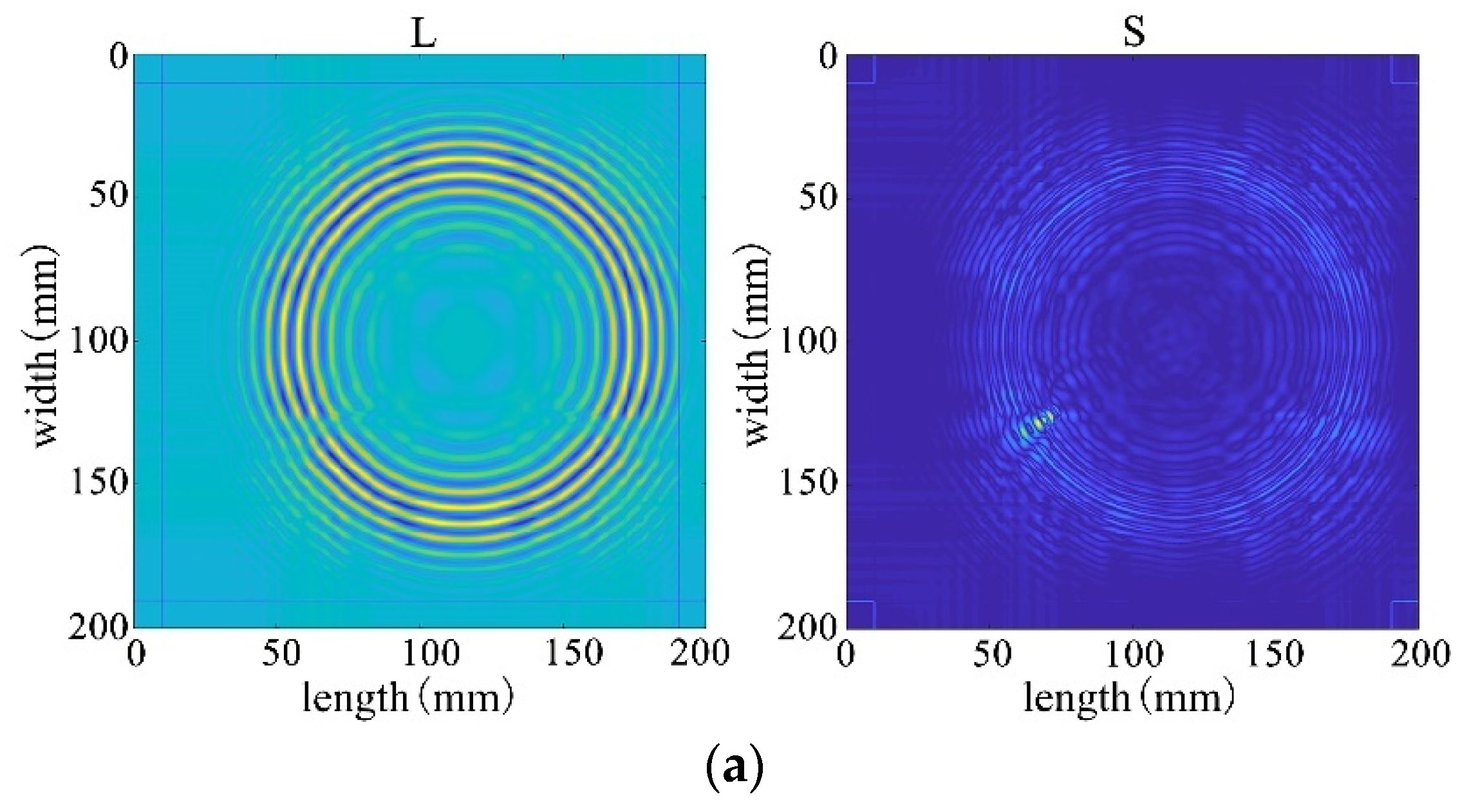
Subsequently, employing the algorithm proposed in this paper for processing, the results from Figure 28 reveal that the decomposition outcomes of this chapter’s algorithm are closer to the ideal. They can accurately separate the low-rank and sparse components of the wavefield image, allocating as much useful information as possible to the low-rank component while avoiding excessive redundant information in the sparse matrix. This achievement facilitates efficient restoration of the low-rank component. Therefore, through comparative analysis between Figure 28 and Figure 29, it is evident that the algorithm proposed in this paper significantly outperforms existing traditional algorithms, better preserving the damaged information.

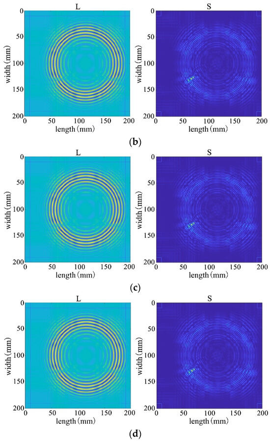
Figure 29.
The decomposition results of the improved algorithm regarding different non-convex penalty functions. (a) NCA-RPCA (ARCTAN) decomposition result. (b) NCA-RPCA (ETP) decomposition result. (c) NCA-RPCA (SCAD) decomposition result. (d) NCA-RPCA (Log) decomposition result.
To further compare the advantages and disadvantages of the NCA-RPCA algorithm proposed in this paper with traditional algorithms, a comparative analysis of time efficiency in handling different types of defects was conducted. As shown in Table 3, traditional algorithms take significantly longer for damage identification, more than ten times longer than the algorithm proposed in this chapter. The proposed algorithm substantially reduces processing time, greatly enhancing SHM’s real-time monitoring efficiency. The reduction in time costs provides a more efficient solution for related application areas, meeting the demands of practical application scenarios.
Table 3.
The processing time of different algorithms.
This study conducts performance evaluations of several algorithms from various aspects, such as the rank of low-rank matrices, decomposition error, and iteration count. The analysis results from Table 4 indicate that the algorithm proposed in this chapter exhibits significant advantages across all metrics. Firstly, in the decomposed low-rank matrices, this chapter’s algorithm demonstrates a higher capability to restore original data information at a lower rank level, showcasing superior information restoration ability. Secondly, the decomposition error is significantly reduced, indicating that the algorithm in this paper more effectively preserves the data’s characteristics. Most importantly, there is a substantial decrease in the number of iterations, highlighting the efficiency and superiority of the algorithm proposed in this paper. These results collectively demonstrate a significant improvement in the overall performance of the algorithm proposed in this paper, providing a more reliable and efficient solution for practical applications in related fields.
Table 4.
The performance comparison of different algorithms.
5.3. Experimental Verification of Wavefield
5.3.1. Experimental Configuration
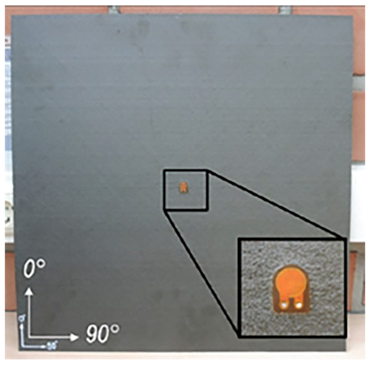
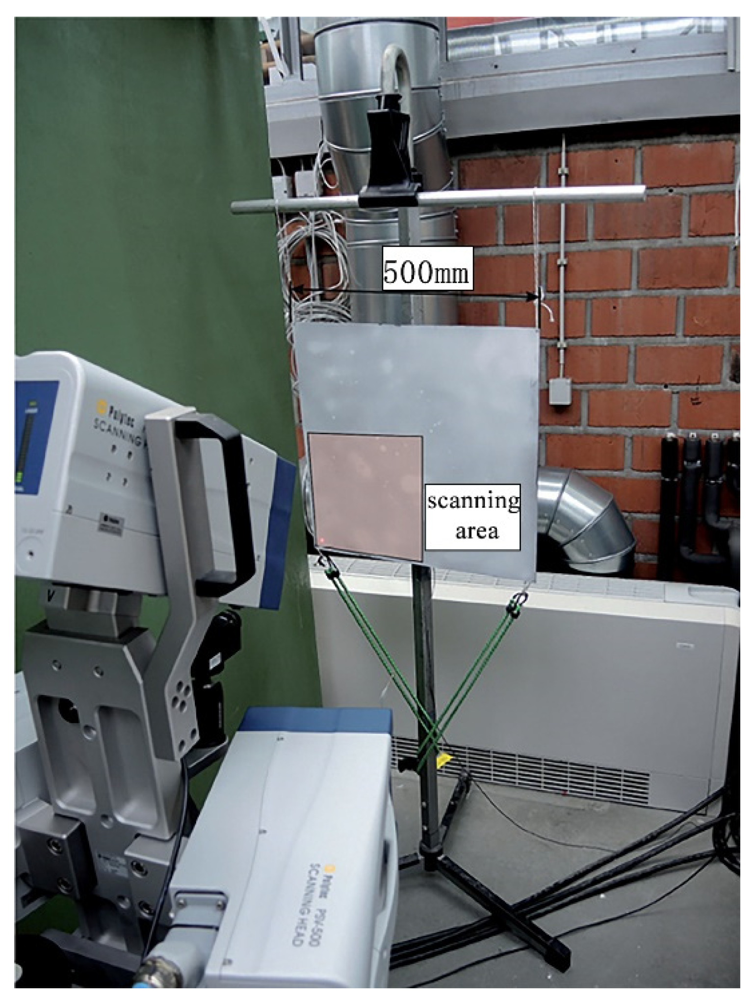
For further validation of the algorithm, a publicly available dataset from the University of Göttingen, Germany, is used in this paper [46]. These data are for a CFRP plate with dimensions of 500 × 500 mm and a thickness of 2 mm with the material properties shown in Table 5, the structure of the plate is shown in Figure 30. A piezoelectric transducer was located in the center of the structural plate for acoustic field measurements. An aluminum disc was mounted on the surface of the CFRP plate using adhesive tape to simulate damage. The excitation signal was a 5-cycle Hanning window-modulated sine wave. The experiment was carried out using a PSV-400-3D from Polytec GmbH (Waldbronn, Germany) for full wavefield measurements. Due to symmetry, only the lower left quarter of the plate was swept. Therefore, the sensor was located in the lower-left corner of the measured wavefield. The experiment is shown in Figure 31.
Table 5.
Material properties of structural plates.
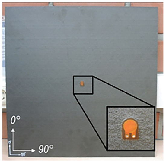
Figure 30.
Experimental thin plate structures.

Figure 31.
Experiment setup for structural plates and laser Doppler vibrometer.
5.3.2. Experimental Results and Analysis
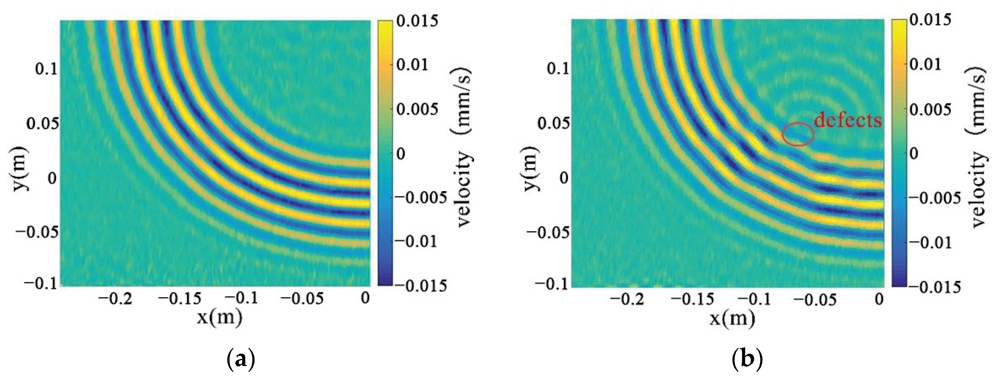
This utilizes the full wavefield image data measured by PSV-400-3D, which is the key to the in-depth study of the real wavefield environment data. The wavefield image data in damage and non-defective cases are extracted respectively, as shown in Figure 32a,b, and processed by different algorithms for comparative analyses to reveal the advantages and disadvantages of the algorithms in dealing with real data.
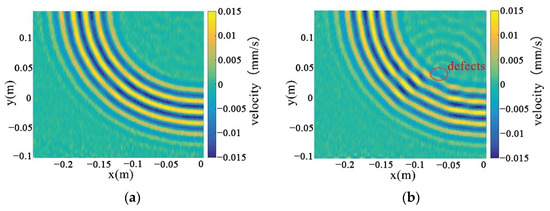
Figure 32.
Full-wavefield image with experimental data. (a) non-defective conditions (b) destructive conditions.
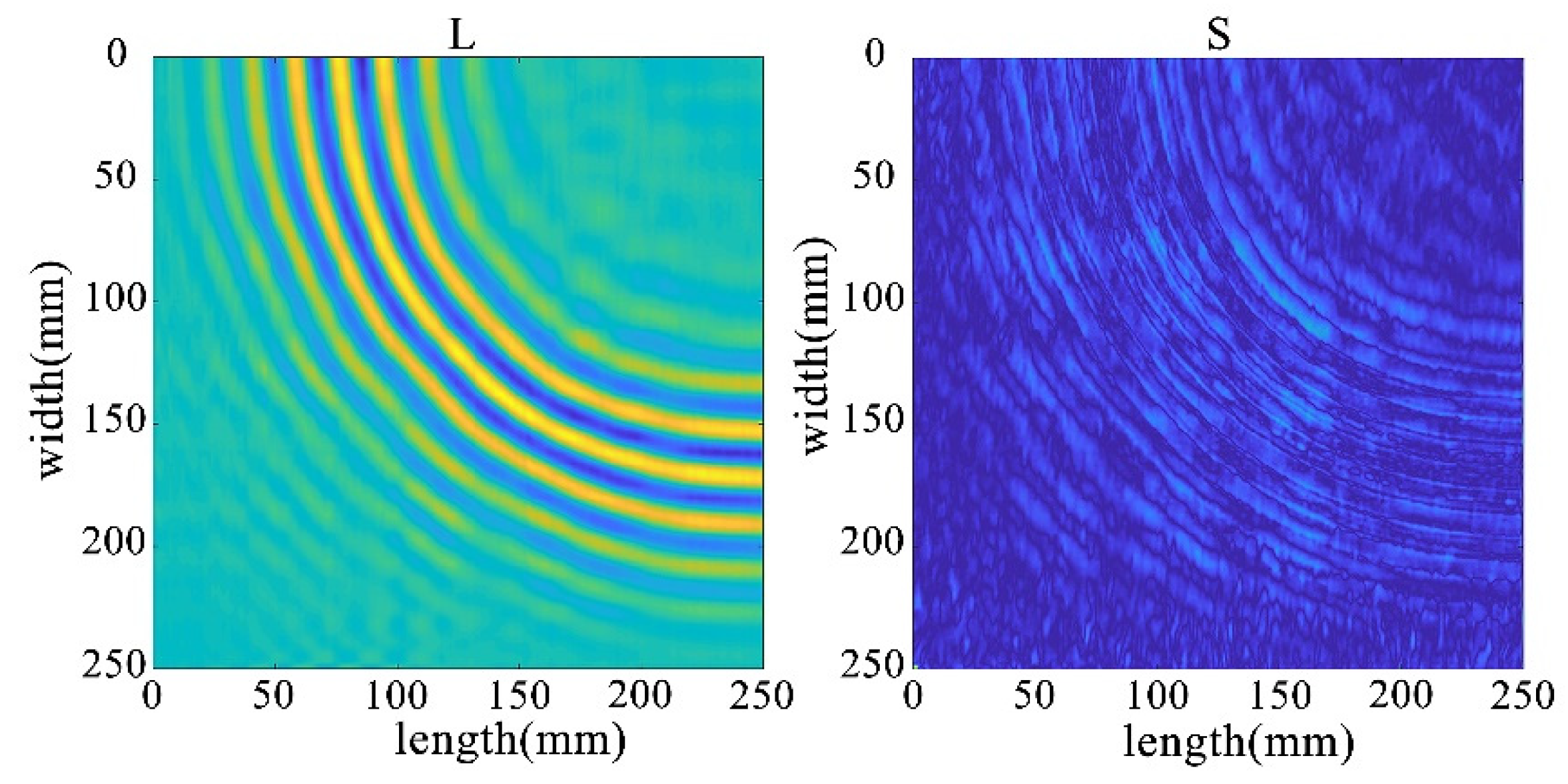
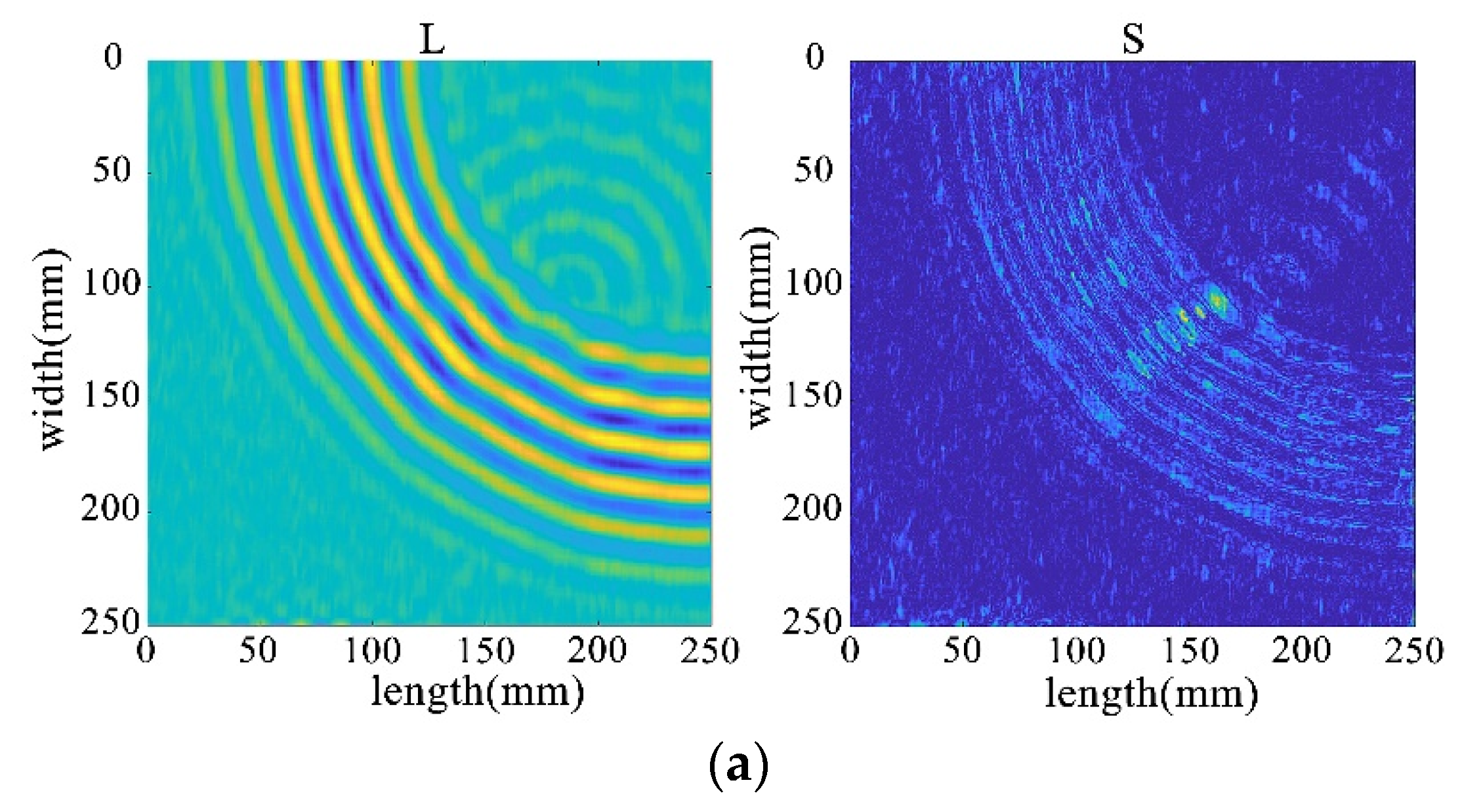
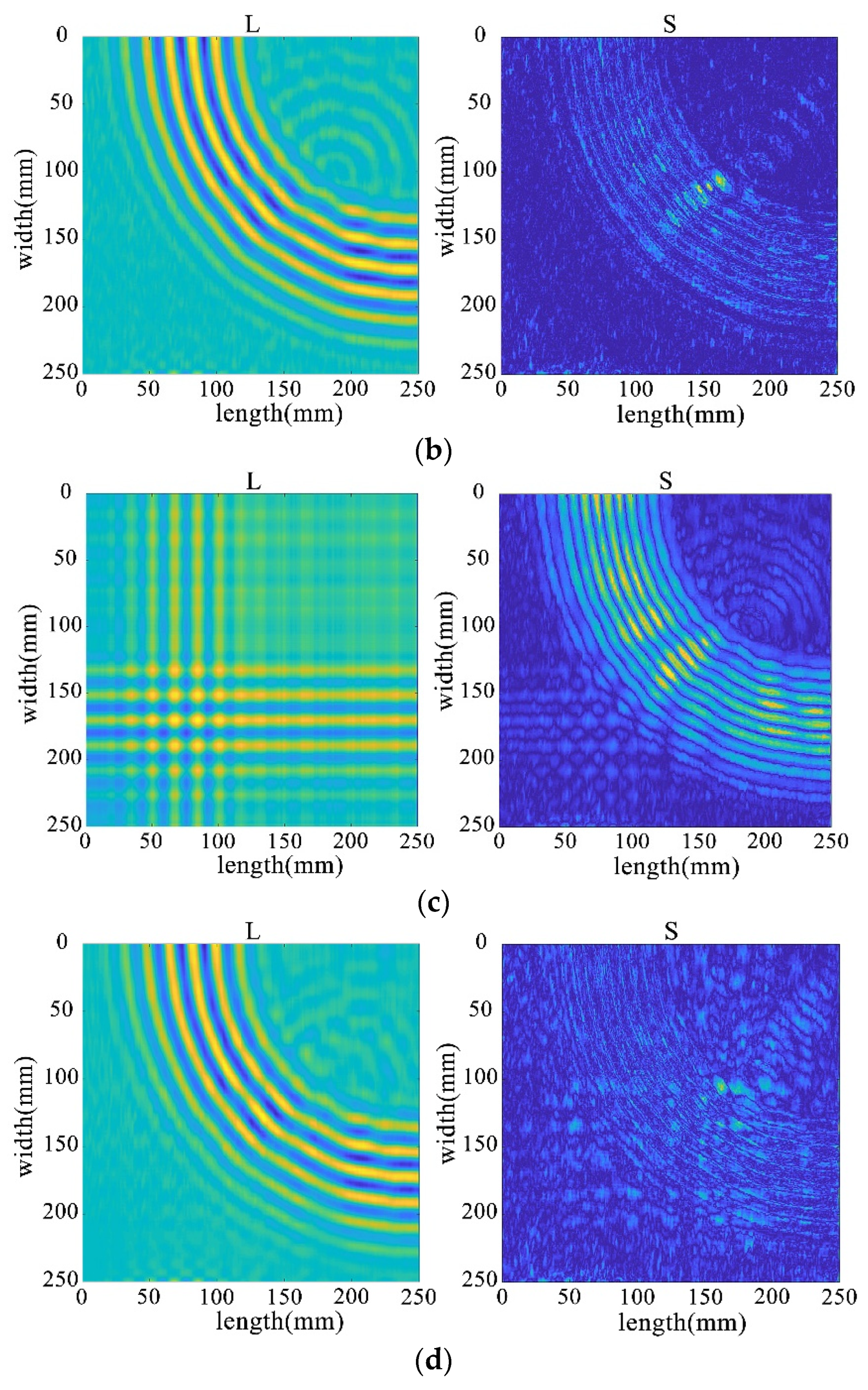
Through the decomposition process of the non-destructive image, it can be seen that the sparse matrix has only noise and no obvious damage points, as shown in Figure 33. From the results in Figure 34 and Figure 35, it can be seen that compared with the processing results under lossless conditions, under lossy conditions, the sparse images decomposed by the rest of the algorithms show obvious damage points, except for the FPCP algorithm (Figure 34c), which still fails to efficiently separate out the useful information from the outliers in this processing, and all of them can accurately decompose the low-rank and sparse images. However, it can be seen in Figure 34d that the RPCA-GD algorithm, although successful in separating useful information and damaged information, is not very effective for the experimental data extracted under complex conditions.

Figure 33.
Full wavefield image decomposition results under non-destructive conditions.
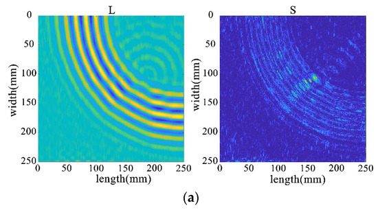
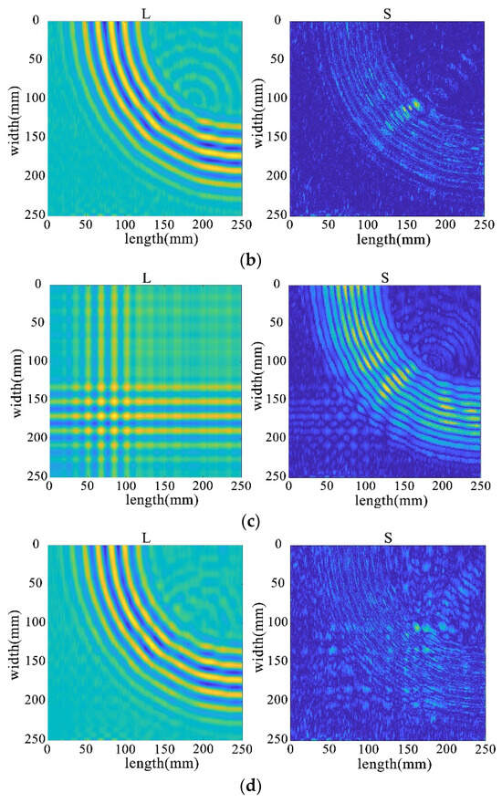
Figure 34.
Decomposition results for traditional algorithms. (a) IALM decomposition results. (b) APG decomposition results. (c) FPCP decomposition results. (d) RPCA-GD decomposition results.
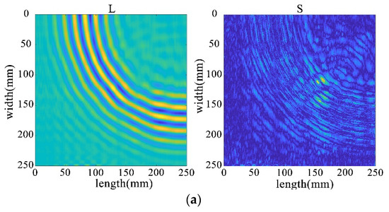
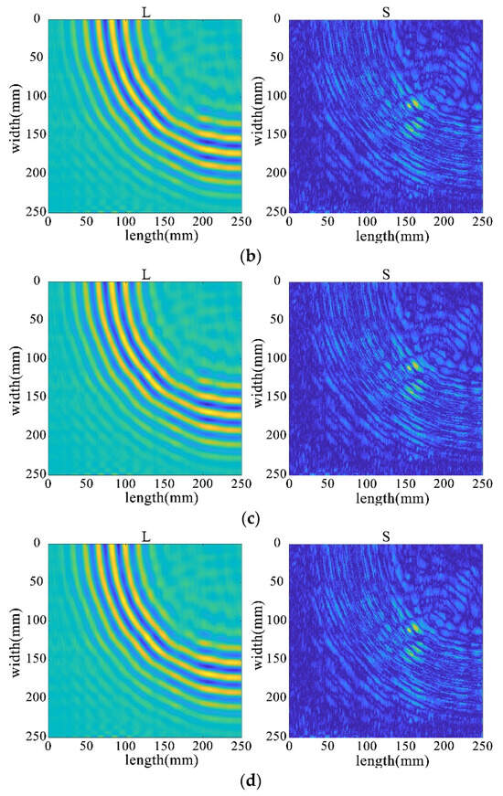
Figure 35.
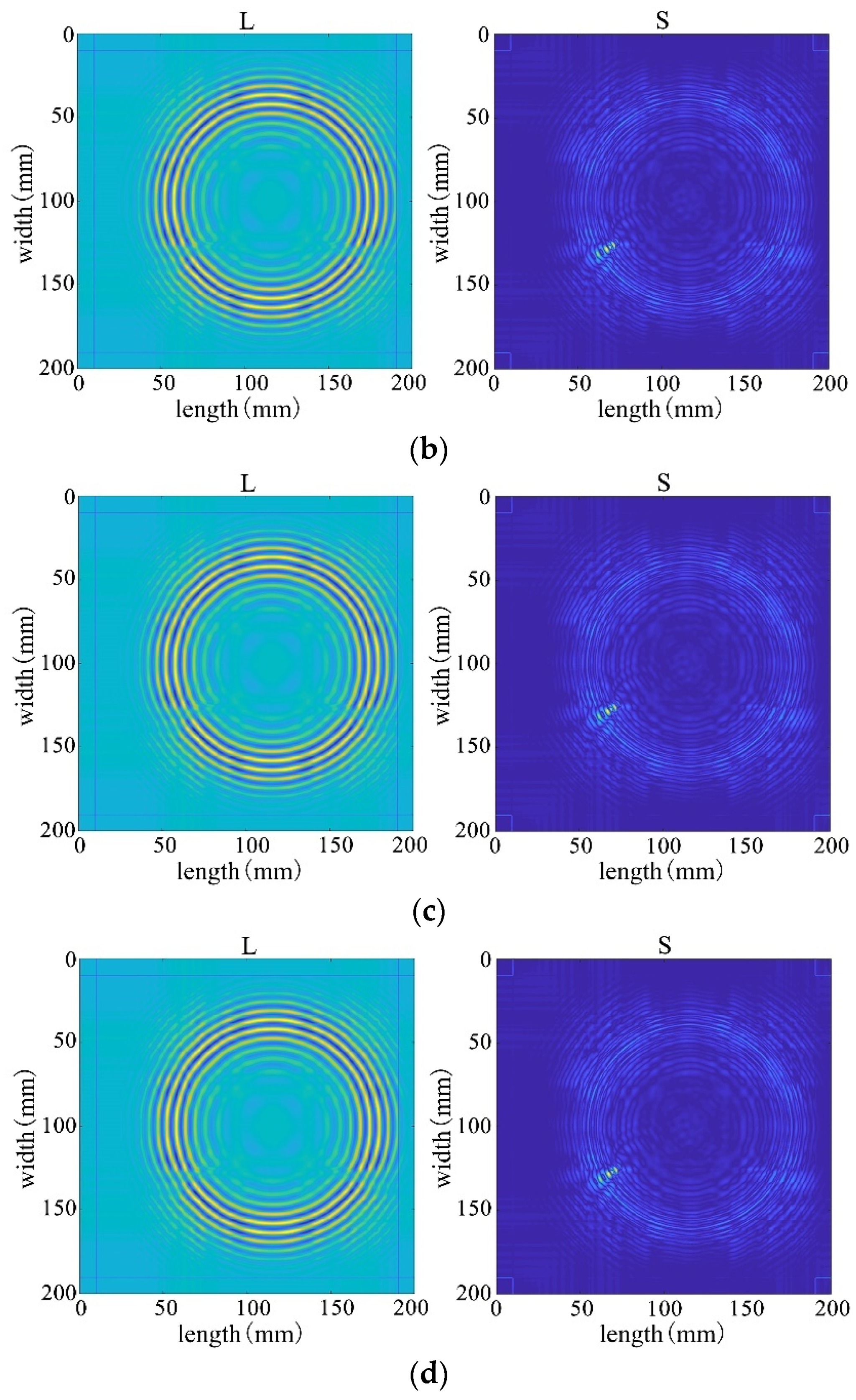
Decomposition results of the improved algorithm with different non-convex penalty functions. (a) NCA-RPCA (ARCTAN) decomposition results. (b) NCA-RPCA (ETP) decomposition results. (c) NCA-RPCA (Log) decomposition results. (d) NCA-RPCA (SCAD) decomposition results.
To compare the advantages and disadvantages of the algorithm effects in depth, this study further evaluates them comprehensively from several aspects, including the rank of the low-rank matrix, the decomposition error, the number of iterations, and the processing time, etc., which are interrelated with each other, and together constitute a comprehensive framework for the evaluation of the algorithms’ performances.
According to the results in Table 6, for the experimental real data, the algorithm designed in Section 4 firstly separates the low-rank matrices with a rank of seven, which possesses a much lower rank and is about three times lower than the traditional method, indicating that it can restore the original data information at a much lower rank level. Secondly, the decomposition error is also significantly reduced by an order of magnitude, and the number of iterations and processing time are also drastically reduced, which greatly improves the real-time monitoring efficiency of SHM. These comprehensive results fully demonstrate the advantages of this paper’s algorithm in several aspects, highlighting the superiority of the improved algorithm in processing full-wavefield experimental data, which not only provides more accurate damage identification but also possesses high monitoring efficiency, providing a reliable solution for applications in the field of structural health monitoring.
Table 6.
The comparative analysis of various algorithms’ performance.
6. Summary
6.1. Conclusions
In summary, this study has investigated and proposed the NCA-RPCA algorithm for wavefield image-based damage detection. The algorithm combines the advantages of non-convex approximation, robust principal component analysis, and alternating optimization techniques. Through extensive experiments and analyses, the algorithm’s effectiveness and superiority in handling various scenarios of wavefield images have been demonstrated. The NCA-RPCA algorithm effectively separates wavefield images into low-rank and sparse components, enabling accurate identification and localization of structural damage. It exhibits robustness to noise and outlier interference, making it particularly suitable for real-world applications where data can be complex and noisy.
By processing damaged images, this algorithm demonstrates the capability to swiftly and accurately detect damaged areas within the images. It effectively identifies anomalous regions and provides reliable diagnostic outcomes. Building upon its success in single defect detection, the algorithm also showcases strong scalability. It remains effective when dealing with multiple defects, efficiently locating and marking multiple areas of damage rather than being limited to a single defect. This emphasizes the algorithm’s robustness and adaptability in handling intricate scenarios. Such achievements hold significant practical implications in the field of defect detection. In numerous real-world applications, multiple defects in various locations are common. The success of this algorithm validates its reliability in real-life situations, underscoring its value for practical deployment.
Furthermore, the algorithm’s adaptability to different types, sizes, and positions of defects has been thoroughly examined. It excels in detecting both single and multiple defects, showcasing its versatility and robustness in challenging situations. Compared to existing methods, the NCA-RPCA algorithm exhibits higher efficiency, faster convergence, and improved accuracy in detecting anomalies within wavefield images.
In summary, this algorithm excels in both single defect detection and multiple defect detection, showcasing remarkable advantages over traditional methods. Its strong detection capability and application potential are evident, signifying its effectiveness. This advancement contributes to the progression of damage detection techniques in structural health monitoring. The strengths and achievements of the NCA-RPCA algorithm provide a solid foundation for its practical implementation across various industries, offering promising prospects for enhancing tasks such as data analysis, anomaly detection, and pattern recognition.
6.2. Problem Analysis and Prospects
Although the algorithm shows promising results in identifying structural damage and has advantages over traditional methods, there are still some limitations. These mainly include the following aspects.
The first is that this study is limited to damage identification only and does not complete the work of damage localization, which can be followed up by using some localization algorithms to locate the specific horizontal and vertical coordinates of the damage.
The second is that if two defects are far away from each other on the image, it is difficult to accurately capture the information about both defects at the same time. To overcome this challenge, we can apply a period of continuous Lamb waves to obtain more information about defect detection. By continuous Lamb wave excitation, more information can be introduced in the image, including multiple angles and directions of excitation. This will make the information in the damaged region richer and more diversified, which will help improve the defect detection rate and accuracy. At the same time, the continuous excitation can cover a larger area, enabling a more comprehensive view of the anomalies in the image and avoiding missing more distant damage.
Finally, we can further explore the algorithm regarding the choice of non-convex penalty functions. Different non-convex penalty functions may have an impact on the excellence of the algorithm, so comparative experiments can be conducted to try different penalty functions and observe their effects on damage recognition. Such research can help us to find a more suitable penalty function for the problem characteristics and further improve the accuracy and robustness of the algorithm.
Author Contributions
Conceptualization, D.L.; Methodology, Y.Z.; Software, Y.Z.; Validation, L.Y.; Formal analysis, Y.Z.; Resources, X.J.; Data curation, Y.Z.; Writing—original draft, A.L.; Visualization, G.S. All authors have read and agreed to the published version of the manuscript.
Funding
This research was funded by the National Natural Science Foundation of China (Grant no. 51405409), Key research project of Jiangsu grant number [BE2016056], Primary Research and Development Plan of Jiangsu Province (Social Development) (BE2019649), State Key Laboratory of Acoustics, Chinese Academy of Sciences (SKLA201913), the Fundamental Research Funds for the Central Universities (2018B04514, B200202212), Technology Support Plan (Social Development) Project Foundation of Changzhou (Grant No. CE20215017), and China Scholarship Council (202006715050).
Institutional Review Board Statement
Not applicable.
Informed Consent Statement
Not applicable.
Data Availability Statement
The data presented in this study are available on request from the corresponding author. (for legal/ethical reasons).
Conflicts of Interest
The authors declare no conflict of interest.
References
- Raghavan, A.; Cesnik, C.E.S. Review of guided-wave structural health monitoring. Shock. Vib. Dig. 2007, 39, 91–116. [Google Scholar] [CrossRef]
- Rose, J.L. A baseline and vision of ultrasonic guided wave inspection potential. J. Press. Vessel Technol. 2002, 124, 273–282. [Google Scholar] [CrossRef]
- Lowe, M.; Cawley, P. Long Range guided Wave Inspection Usage—Current Commercial Capabilities and Research Directions; Technical Report; Department of Mechanical Engineering, Imperial College London: London, UK, 2006; pp. 1–40. [Google Scholar]
- Mitra, M.; Gopalakrishnan, S. Smart Materials and Structures Guided wave based structural health monitoring: A review. Smart Mater. Struct. 2016, 27, 053001. [Google Scholar] [CrossRef]
- Boller, C.; Chang, F.-K.; Fujino, Y. Encyclopedia of Structural Health Monitoring; Wiley: Hoboken, NJ, USA, 2009. [Google Scholar]
- Chen, X.; Li, X.; Wang, S.; Yang, Z.; Chen, B.; He, Z. Composite damage detection based on redundant second-generation wavelet transform and fractal dimension tomography algorithm of Lamb wave. IEEE Trans. Instrum. Meas. 2013, 62, 1354–1363. [Google Scholar] [CrossRef]
- Li, X.; Yang, Z.; Zhang, H.; Du, Z.; Chen, X. Crack growth sparse pursuit for wind turbine blade. Smart Mater. Struct. 2014, 24, 015002. [Google Scholar] [CrossRef]
- Mesnil, O.; Yan, H.; Ruzzene, M.; Paynabar, K.; Shi, J. Fast wavenumber measurement for accurate and automatic location and quantifification of defect in composite. Struct. Health Monitor. 2016, 15, 223–234. [Google Scholar] [CrossRef]
- Staszewski, W.; Lee, B.C.; Traynor, R. Fatigue crack detection in metallic structures with Lamb waves and 3D laser vibrometry. Meas. Sci. Technol. 2007, 18, 727. [Google Scholar] [CrossRef]
- Sriram, P.; Craig, J.I.; Hanagud, S. Scanning laser Doppler techniques for vibration testing. Exp. Tech. 1992, 16, 21–26. [Google Scholar] [CrossRef]
- Xu, H.; Caramanis, C.; Sanghavi, S. Robust PCA via outlier pursuit. IEEE Trans. Inf. Theory 2012, 58, 3047–3064. [Google Scholar] [CrossRef]
- Nie, Z.; Guo, E.; Li, J.; Hao, H.; Ma, H.; Jiang, H. Bridge condition monitoring using fixed moving principal component analysis. Struct. Control Health Monit. 2020, 27, e2535. [Google Scholar] [CrossRef]
- Akintunde, E.; Azam, S.E.; Rageh, A.; Linzell, D. Full scale bridge damage detection using sparse sensor networks, principal component analysis, and novelty detection. Proceedings 2019, 42, 1. [Google Scholar] [CrossRef]
- Mújica, L.E.; Ruiz, M.; Pozo, F.; Rodellar, J.; Güemes, A. A structural damage detection indicator based on principal component analysis and statistical hypothesis testing. Smart Mater. Struct. 2013, 23, 025014. [Google Scholar] [CrossRef]
- Azim, M.R.; Gül, M. Data-driven damage identification technique for steel truss railroad bridges utilizing principal component analysis of strain response. Struct. Infrastruct. Eng. 2020, 17, 1019–1035. [Google Scholar] [CrossRef]
- Yang, P.; Hsieh, C.-J.; Wang, J.-L. History PCA: A new algorithm for streaming PCA. arXiv 2018, arXiv:1802.05447. [Google Scholar]
- Burrello, A.; Marchioni, A.; Brunelli, D.; Benatti, S.; Mangia, M.; Benini, L. Embedded streaming principal components analysis for network load reduction in structural health monitoring. IEEE Internet Things J. 2021, 8, 4433–4447. [Google Scholar] [CrossRef]
- Moallemi, A.; Burrello, A.; Brunelli, D.; Benini, L. Exploring Scalable, Distributed Real-Time Anomaly Detection for Bridge Health Monitoring. IEEE Internet Things J. 2022, 9, 17660–17674. [Google Scholar] [CrossRef]
- Flexa, C.; Gomes, W.; Sales, C. Data Normalization in Structural Health Monitoring by Means of Nonlinear Filtering. In Proceedings of the 2019 8th Brazilian Conference on Intelligent Systems (BRACIS), Salvador, Brazil, 15–18 October 2019; pp. 204–209. [Google Scholar]
- Anaya, M.; Tibaduiza, D.A.; Forero, E.; Castro, R.; Pozo, F. An acousto-ultrasonics pattern recognition approach for damage detection in wind turbine structures. In Proceedings of the 2015 20th Symposium on Signal Processing, Images and Computer Vision (STSIVA), Bogota, Colombia, 2–4 September 2015; pp. 1–5. [Google Scholar]
- Garcia-Sanchez, D.; Fernandez-Navamuel, A.; Sánchez, D.Z.; Alvear, D.; Pardo, D. Bearing assessment tool for longitudinal bridge excellence. J. Civ. Struct. Health Monit. 2020, 10, 1023–1036. [Google Scholar] [CrossRef]
- Calderano, P.; De Marins, D.B.; Ayala, H. A comparison of Feature Extraction Methods for Crack and Ice Monitoring in Wind Turbine Blades: System Identification and Matrix Decomposition. In Proceedings of the 2022 30th Mediterranean Conference on Control and Automation (MED), Vouliagmeni, Greece, 28 June–1 July 2022; pp. 779–784. [Google Scholar]
- Candès, J.; Li, X.; Ma, Y.; Wright, J. Robust principal component analysis? J. ACM 2011, 58, 11. [Google Scholar] [CrossRef]
- Ma, S.; Aybat, N.S. Efficient optimization algorithms for robust principal component analysis and its variants. Proc. IEEE 2018, 106, 1411–1426. [Google Scholar] [CrossRef]
- Chen, Y.; Wang, Y.; Li, M.; He, G. Augmented lagrangian alternating direction method for low-rank minimization via non-convex approximation. Signal Image Video Process. 2017, 11, 1271–1278. [Google Scholar] [CrossRef]
- Balcan, M.; Liang, Y.; Song, Z.; Woodruff, D.; Zhang, H. Non-convex matrix completion and related problems via strong duality. J. Mach. Learn. Res. 2019, 20, 1–56. [Google Scholar]
- Yang, Z.; Fan, L.; Yang, Y.; Yang, Z.; Gui, G. Generalized singular value thresholding operator based nonconvex low-rank and sparse decomposition for moving object detection. J. Frankl. Inst. 2019, 356, 10138–10154. [Google Scholar] [CrossRef]
- Wen, F.; Ying, R.; Liu, P.; Truong, T.-K. Nonconvex regularized robust PCA using the proximal block coordinate descent algorithm. IEEE Trans. Signal Process. 2019, 67, 5402–5416. [Google Scholar] [CrossRef]
- Kang, Z.; Peng, C.; Cheng, Q. Robust PCA via nonconvex rank approximation. In Proceedings of the IEEE International Conference on Data Mining, Atlantic City, NJ, USA, 14–17 November 2015; pp. 211–220. [Google Scholar]
- Li, X.; Ding, S.; Tan, B. Accurate defect detection in thin-wall structures with transducer networks via outlier elimination. IEEE Sens. J. 2018, 18, 9619–9628. [Google Scholar] [CrossRef]
- Dong, Y.; Wang, J.; Li, C.; Liu, Z.; Xi, J. Fusing multilevel deep features for fabric defect detection based NTV-RPCA. IEEE Access 2020, 8, 161872–161883. [Google Scholar] [CrossRef]
- Ebrahimi, S.; Fleuret, J.; Klein, M.; Théroux, L.-D.; Georges, M.; Ibarra-Castanedo, C.; Maldague, X. Robust Principal Component Thermography for Defect Detection in Composites. Sensors 2021, 21, 2682. [Google Scholar] [CrossRef]
- Wang, J.; Xu, G.; Li, C.; Wang, Z.; Yan, F. Surface defects detection using non-convex total variation regularized RPCA with kernelization. IEEE Trans. Instrum. Meas. 2021, 70, 5007013. [Google Scholar] [CrossRef]
- Wang, F.; Wang, L.; Wen, Y.; Ha, F.; Lu, J.; Jiao, W. Intelligent Diesel Engine Fault Diagnosis Method Based on Time-Frequency-Nonconvex Robust Principal Component Analysis. In Proceedings of the ICSMD, Harbin, China, 30 November–2 December 2022; pp. 1–5. [Google Scholar]
- Ning, W.; Wang, Y. Propagation of Lamb waves in three-layered solid composite media. Acta Acust. 1996, 21, 414–420. [Google Scholar]
- ElTantawy, A.; Shehata, M.S. KRMARO: Aerial detection of small-size ground moving objects using kinematic regularization and matrix rank optimization. IEEE Trans. Circuits Syst. Video Technol. 2018, 29, 1672–1686. [Google Scholar] [CrossRef]
- Bertsekas, D.P. Constrained Optimization and Lagrange Multiplier Methods; Academic Press: Cambridge, MA, USA, 2014. [Google Scholar]
- Zhang, S.; Zhao, J. Through-wall radar imaging algorithm based on IALM. J. Comput. Eng. Appl. 2021, 57, 77–83. [Google Scholar]
- Gasso, G.; Rakotomamonjy, A.; Canu, S. Recovering sparse signals with a certain family of nonconvex penalties and DC programming. IEEE Trans. Signal Process. 2009, 57, 4686–4698. [Google Scholar] [CrossRef]
- Mei, X.; Ma, Y.; Fan, F.; Li, C.; Liu, C.; Huang, J.; Ma, J. Infrared ultraspectral signature classification based on a restricted Boltzmann machine with sparse and prior constraints. Int. J. Remote Sens. 2015, 36, 4724–4747. [Google Scholar] [CrossRef]
- Gao, C.; Wang, N.; Yu, Q.; Zhang, Z. A feasible nonconvex relaxation approach to feature selection. Proc. AAAI Conf. Artif. Intell. 2011, 25, 356–361. [Google Scholar] [CrossRef]
- Li, F.R. Variable Selection via Nonconcave Penalized Likelihood and its Oracle Properties. Publ. Am. Stat. Assoc. 2001, 96, 1348–1360. [Google Scholar]
- Donoho, D.L. De-noising by soft-thresholding. IEEE Trans. Inf. Theory 1995, 41, 613–627. [Google Scholar] [CrossRef]
- Hindmarsh, A.C.; Brown, P.N.; Grant, K.E.; Lee, S.L.; Serban, R.; Shumaker, D.E.; Woodward, C.S. SUNDIALS: Suite of nonlinear and differential/algebraic equation solvers. ACM Trans. Math. Softw. 2005, 31, 363–396. [Google Scholar] [CrossRef]
- Moser, F.; Jacobs, L.J.; Qu, J. Modeling elastic wave propagation in waveguides with the finite element method. NDT E Int. 1999, 32, 225–234. [Google Scholar] [CrossRef]
- Moll, J.; Kathol, J.; Fritzen, C.P.; Moix-Bonet, M.; Rennoch, M.; Koerdt, M.; Herrmann, A.S.; Sause, M.G.; Bach, M. Open Guided Waves-Online Platform for Ultrasonic Guided Wave Measurements. Struct. Health Monit. 2018, 18, 1903–1914. [Google Scholar] [CrossRef]
- ISO 527-5:2009; Determination of Tensile Properties—Part 5: Test Conditions for Unidirectional Fiber-Reinforced Plastic Composites. ISO: Geneva, Switzerland, 2009. Available online: https://scholar.google.com/scholar_lookup?title=Determination+of+Tensile+Properties%E2%80%94Part+5:+Test+Conditions+for+Unidirectional+Fiber-Reinforced+Plastic+Composites&author=ISO+527-5:2009&publication_year=2009 (accessed on 10 May 2024).
- ISO 14129:1997; Fibre-Reinforced Plastic Composites—Determination of the In-Plane Shear Stress/Shear Strain Response, Including the In-Plane Shear Modulus and Strength, by the Plus or Minus 45 Degree Tension Test Method. International Organization for Standardization: Geneva, Switzerland, 1997. Available online: https://www.iso.org/standard/23641.html (accessed on 10 May 2024).


Disclaimer/Publisher’s Note: The statements, opinions and data contained in all publications are solely those of the individual author(s) and contributor(s) and not of MDPI and/or the editor(s). MDPI and/or the editor(s) disclaim responsibility for any injury to people or property resulting from any ideas, methods, instructions or products referred to in the content. |
© 2024 by the authors. Licensee MDPI, Basel, Switzerland. This article is an open access article distributed under the terms and conditions of the Creative Commons Attribution (CC BY) license (https://creativecommons.org/licenses/by/4.0/).