Abstract
The discrete element method (DEM) is a vital numerical approach for analyzing the mechanical behavior of elastoplastic wet sand. However, parameter uncertainty persists within the mapping between constitutive relationships and inherent model parameters. We propose a Parameter calibration neural network based on Attention, Retention, and improved Transformer for Sequential data (PartsNet), which effectively captures the nonlinear mechanical behavior of wet sand and obtains the optimal parameter combination for the Edinburgh elasto-plastic adhesion constitutive model. Variational autoencoder-based principal component ordering is employed by PartsNet to reduce the high-dimensional dynamic response and extract critical parameters along with their weights. Gated recurrent units are combined with a novel sparse multi-head attention mechanism to process sequential data. The fusion information is delivered by residual multilayer perceptron, achieving the association between sequential response and model parameters. The errors in response data generated by calibrated parameters are quantified by PartsNet based on adaptive differentiation and Taylor expansion. Remarkable calibration capabilities are exhibited by PartsNet across six evaluation indicators, surpassing seven other deep learning approaches in the ablation test. The calibration accuracy of PartsNet reaches 91.29%, and MSE loss converges to 0.000934. The validation experiments and regression analysis confirmed the generalization capability of PartsNet in the calibration of wet sand. The improved sparse attention mechanism optimizes multi-head attention, resulting in a convergence speed of 21.25%. PartsNet contributes to modeling and simulating the precise mechanical properties of complex elastoplastic systems and offers valuable insights for diverse engineering applications.
1. Introduction
The nonlinear mechanical characteristics of elastoplastic wet sand are ubiquitous in nature and allows it to be used in industrial processing, such as in feed industries [1], agricultural engineering, and biosystems engineering [2,3,4,5,6]. Elastoplastic wet sand formed through accumulation and cementation deviates from the fundamental assumption of continuum mechanics, making the discrete element method (DEM) the primary method for scholars to comprehend its properties. One critical bottleneck that impedes the development and deployment of the DEM is establishing precise mapping between macroscopic mechanical constitutive relationships and microscopic model parameters [7]. Moreover, numerous internal parameters such as the contact plasticity ratio cannot be determined through experimental measurements, and some of these parameters lack direct physical significance in elastoplastic mechanics. The accuracy of model parameters determines the confidence level of the DEM simulation results. Addressing the parameter identification in the DEM constitutes a prerequisite to overcome the aforementioned bottleneck.
Parameter calibration [8,9,10,11,12,13] is an effective method for addressing unidentifiability in parameters and their combinations, with optimization-based techniques being one common approach. The challenge in parameter calibration is identifying meaningful parameter combinations in high-dimensional and highly coupled parameter spaces that can accurately perform numerical simulations. Schmidt and Lipson [14] define meaningful functionalities as those that strike a balance between accuracy and complexity. Model-driven and data-driven technologies [15] are two main research paradigms oriented to parameter calibration. The optimization efficiency of the former depends on the discrepancies between the predicted constitutive model and real systems. Due to the limited expressive ability of the models, the information from real systems is dimensionally reduced, resulting in the natural loss of information during the modeling process. Data-driven strategies use the inherent connections in the data to create more precise parameter combinations, which reduces the need for prior knowledge and enhances the interpretability of the models [16]. Data-driven technologies have advanced significantly during the past two decades along with the emergence of deep learning [17,18]. Horni et al. [19] demonstrated the generalization of deep learning by highlighting, with a sufficient number of neurons and layers, that deep learning can learn to accurately map any number of inputs to any number of outputs, enabling it to model nearly anything, including the parameter unidentifiability in the DEM.
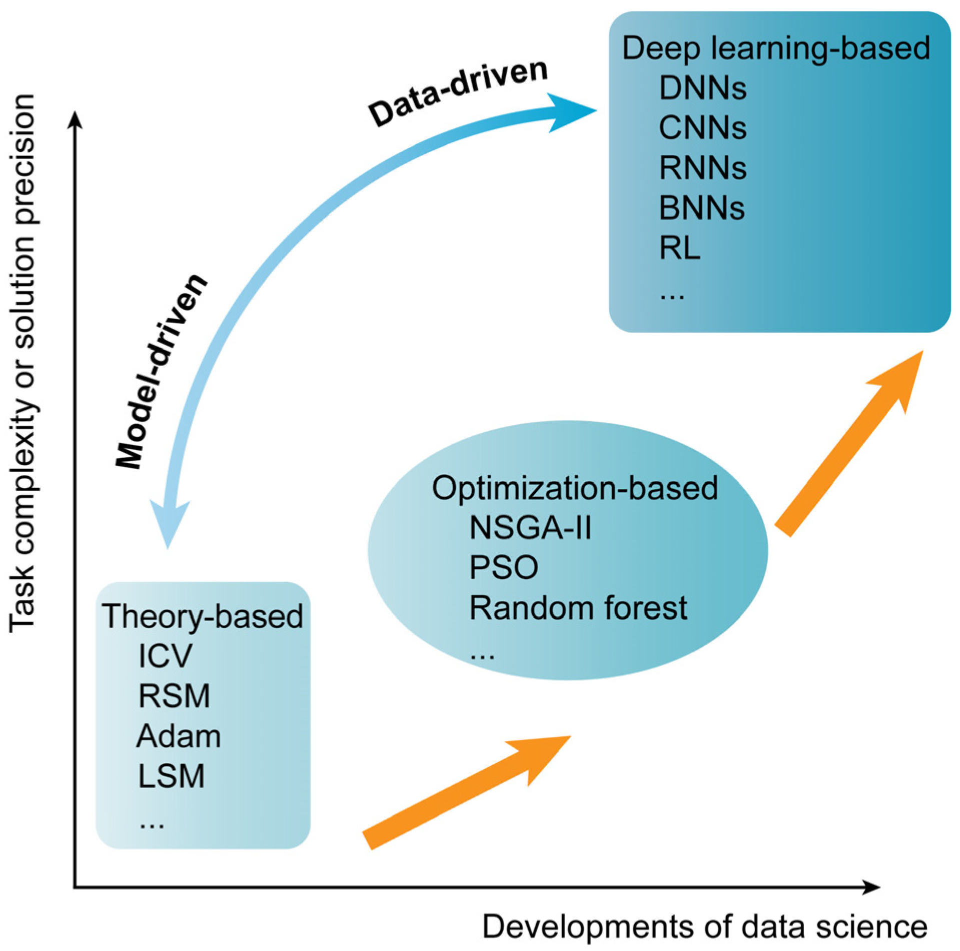
To achieve parameter calibration correctly, researchers have undertaken exploratory works in three aspects, as outlined in Figure 1. The first aspect involves theory-based methods, which utilize sensitivity analysis or the Plackett–Burman analysis [5] to reduce parameter dimensions. Subsequently, iterative cross-analysis [20], response surface methodology [21], adaptive moment estimation [22], and the least squares method [23] are employed for parameter calibration. However, theory-based methods have limited modeling capabilities for nonlinear systems. The assumptions and restrictions on the parameter space may lead to convergence on a solution domain that cannot cover all parameter combinations, making it difficult to achieve parallel calibration for a large number of parameters. The second aspect partially addresses these challenges by applying statistical optimization algorithms. Do et al. [24] proposed a parameter calibration method using nondominated Sorting Genetic Algorithm II, achieving a Pareto-optimal balance between the calibration accuracy and speed. Wang et al. [25] pointed out the limitations of empirical methods in parameter calibration and proposed a new method based on an improved Particle Swarm Optimization (PSO) algorithm. Their work indicated that the empirical formula between micro and macro is not reliable. Boikov et al. [26] introduced a strategy based on random forests, which offers advantages in terms of time complexity and incorporates classical machine learning methods into this field. These methods start to possess global search capability and randomness indicators in the parameter space. However, these methods struggle with handling practical constraints such as parameter value ranges and parameter sensitivity, leading to higher computational costs and time consumption. Furthermore, improved heuristic algorithms tend to be dependent on specific problems. In the third aspect, data-driven techniques centered around deep learning showcase its superiority. Deep learning [17] successfully overcomes the prior difficulties by leveraging automated feature extraction and nonlinear modeling. Researchers have applied DNNs (Deep Neural Networks), CNNs (Convolutional Neural Networks), RNNs (Recurrent Neural Networks), and RL (reinforcement learning) to parameter calibration [8,27,28,29], and deep learning frameworks based on Bayesian inference have also been utilized [30].
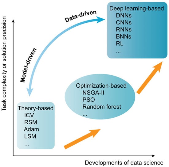
Figure 1.
Data-driven or model-driven parameter calibration methods shown in three aspects.
The existing methods rely on static sampling of the response process to calibrate model parameters. Despite the improving robustness of these methods, the understanding of time-series data from the response process remains inadequate. By utilizing sequence data rather than static sampling points, it becomes possible to learn high-dimensional coupled patterns present in the response data [8]. The generalization of deep learning for sequential data, such as RNNs, is constrained by the long-term dependencies within the data. It is essential to combine the attention mechanism to achieve the ultimate generalization of deep learning in DEM calibration tasks.
This paper proposes an attention retention fusion with a deep learning mechanism, PartsNet, which addresses long-term dependencies by incorporating an improved sparse multi-head self-attention mechanism with a GRU (gated recurrent unit). PartsNet takes the sequence data generated in simulations as the input and the constitutive parameters that need to be calibrated as the output. We study the parameter calibration of the Edinburgh elasto-plastic adhesion (EEPA) model to describe the triaxial compression of wet sand. The calibrated model accurately captures wet sand’s constitutive relationship with exceptional precision. PartsNet obtains the relationship between the macroscopic behavior of wet sand and the microscopic parameters in the EEPA model.
The rest of this paper is organized as follows: The principles, network topology, and implementation details of PartsNet are elucidated in Section 2. In Section 3, we introduce the simulations and experiments conducted on elastoplastic wet sand, along with the calibration results and verification tests of PartsNet for these experiments. In Section 4, we present the parameter calibration results obtained by PartsNet, the ablation experiments, and the error analysis. Finally, some conclusions are given in Section 5.
2. Methodology: PartsNet
In this section, we discuss the three core architectures of PartsNet: GDR-Net, Encoder-Net, and Decoder-Net. These sub-modules collectively establish a systematic framework for parameter calibration.
2.1. General Data Dimensionality Reduction Network (GDR-Net)
The sequence data generated by numerical models are taken as input for PartsNet. Sequence data comprise multidimensional feature parameters, which exhibit non-orthogonality and varying weights. Characterizing a system can be accomplished by calibrating only a few parameters with the most substantial weights and richest information. Previous works [31,32] have mainly relied on principal component analysis (PCA) and its improved algorithms to perform data feature dimensionality reduction. PCA is an unsupervised machine learning approach that may fail to recognize nonlinear connections because of its strict assumptions about the data. This paper proposes a general data dimensionality reduction method based on cross-correlation functions to identify significant features in large datasets. We employ Variational Autoencoders (VAEs) [33] to enhance the feature extraction capability of PartsNet. The sequential data consist of a set of signals.
Definition 1.
For any square-integrable functions,and, represents the cross-correlation of and at m. is subjected to
We use the sigmoid function to normalize the values. For discrete signal functions under investigation, it can be further expressed in the following weak form:
Specially, let K equal 2, and consider the cross-correlation of discrete sequential data at . is subjected to:
The significance of this approach and the weak form lies in establishing a mutual correlation between simulation-generated sequence data and experimentally obtained data, facilitating the labeling process. A higher value of indicates a higher quality of the simulation-generated data, while a lower value indicates the opposite.
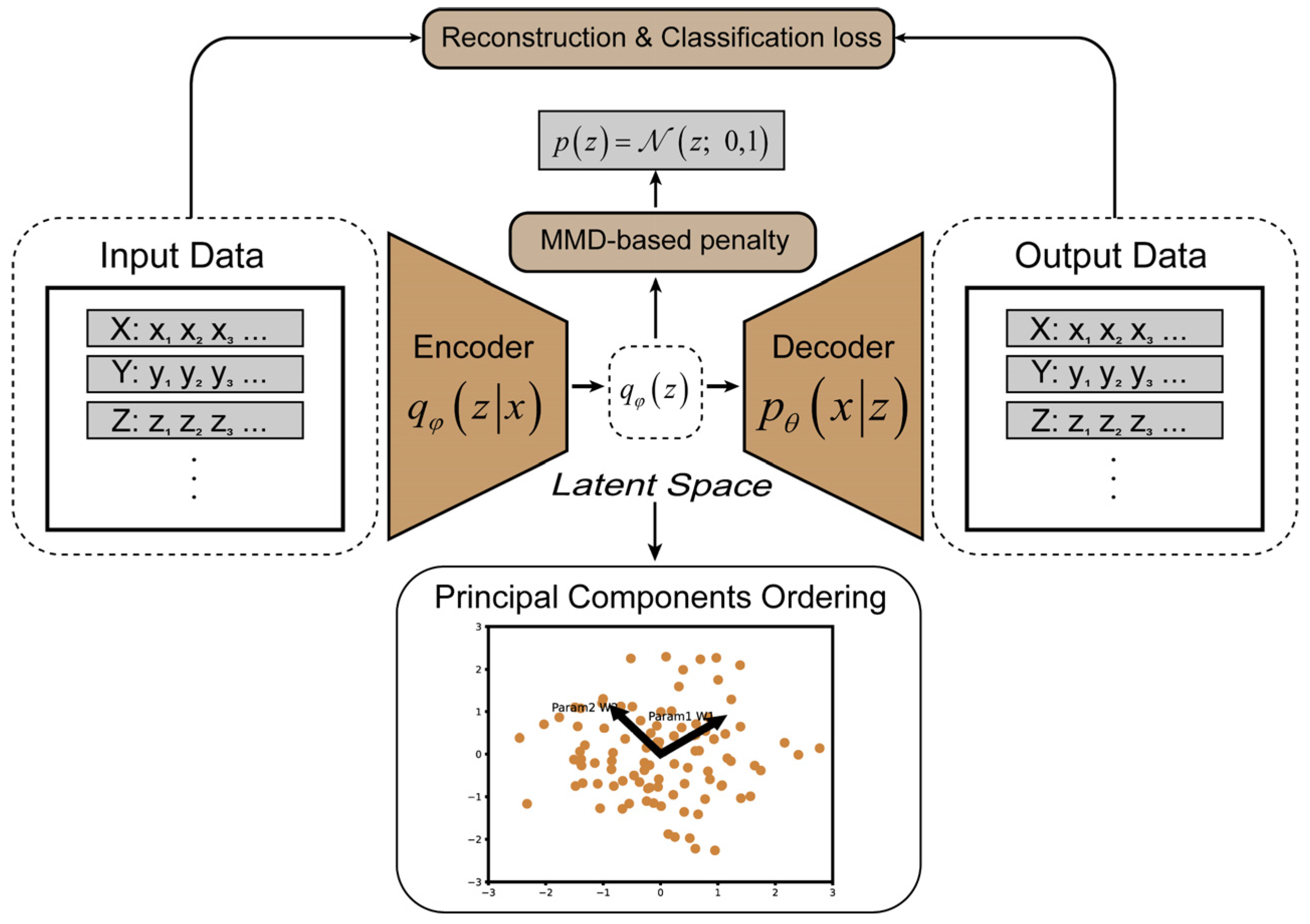
The core of GDR-Net is the use of a VAE for the dimensionality reduction in labeled feature data [34], as shown in Figure 2. A VAE is a generative neural network based on variational Bayesian inference, which addresses the overfitting issue commonly found in traditional autoencoders [35]. The encoder of a generative model uses the input data to learn a compressed form, known as latent variables, while the decoder uses this compressed representation to reconstruct the input. The differences between the original data and the reconstructed data is termed as a reconstruction error, which serves as the optimization objective of autoencoders. The VAE introduces a set of random variables, denoted as z, to represent the latent distribution of the input data and facilitate the generation of new data. The latent model follows a Gaussian distribution, with its mean and variance generated by a parameterized function output by the encoder. The objective of the VAE is to maximize the Evidence Lower Bound (ELBO), which is a lower bound on the log-likelihood of the generative model. The ELBO is defined as follows:
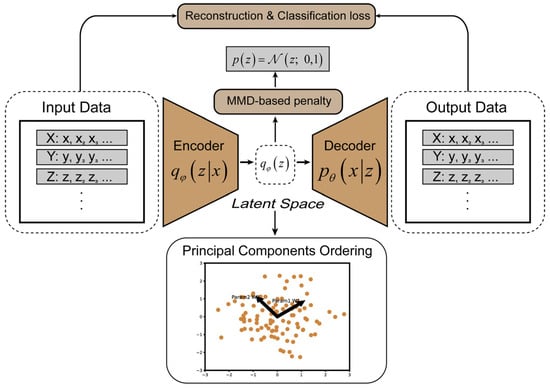
Figure 2.
Architecture of general data dimensionality reduction network (GDR-Net). Encoder with parameter φ takes multi-dimensional features of simulation systems as input, and decoder with parameter θ can act as generator for suggesting new compositions based on learned latent z representation. Low-dimensional features output from latent space obtain their relative weights by principal component ordering.
Here, represents the variational posterior distribution generated by the encoder, represents the generative distribution generated by the decoder, and represents the prior distribution. The first term on the right-hand side corresponds to the reconstruction term, which maximizes the log-likelihood function to measure the similarity between the reconstructed data and the original input. The second term is the Kullback–Leibler (KL) divergence term, which minimizes the KL divergence between distributions and to regularize the distribution of latent variables, ensuring that the learned distribution becomes closer to the prior. During the training process, a multilayer perceptron structure is employed.
Binary Cross-Entropy Loss (BCELoss) is utilized to measure the discrepancy between the predicted data and the original data in terms of labels.
Here, represents the actual quality of the sequence data, which is typically the output of a simulation process, and represents the probability predicted by the model that the data are a positive sample. GDR-Net achieves the learning process by minimizing the negative ELBO and BCELoss.
While a VAE can achieve data dimensionality reduction, it cannot explicitly express the weights of different dimensional features on the results. In this study, a principal component ordering model-based PCA is utilized to handle the features learned in the latent space. This combined approach ensures that GDR-Net can capture crucial features from high-dimensional data and further determine their weights.
2.2. Encoder-Net
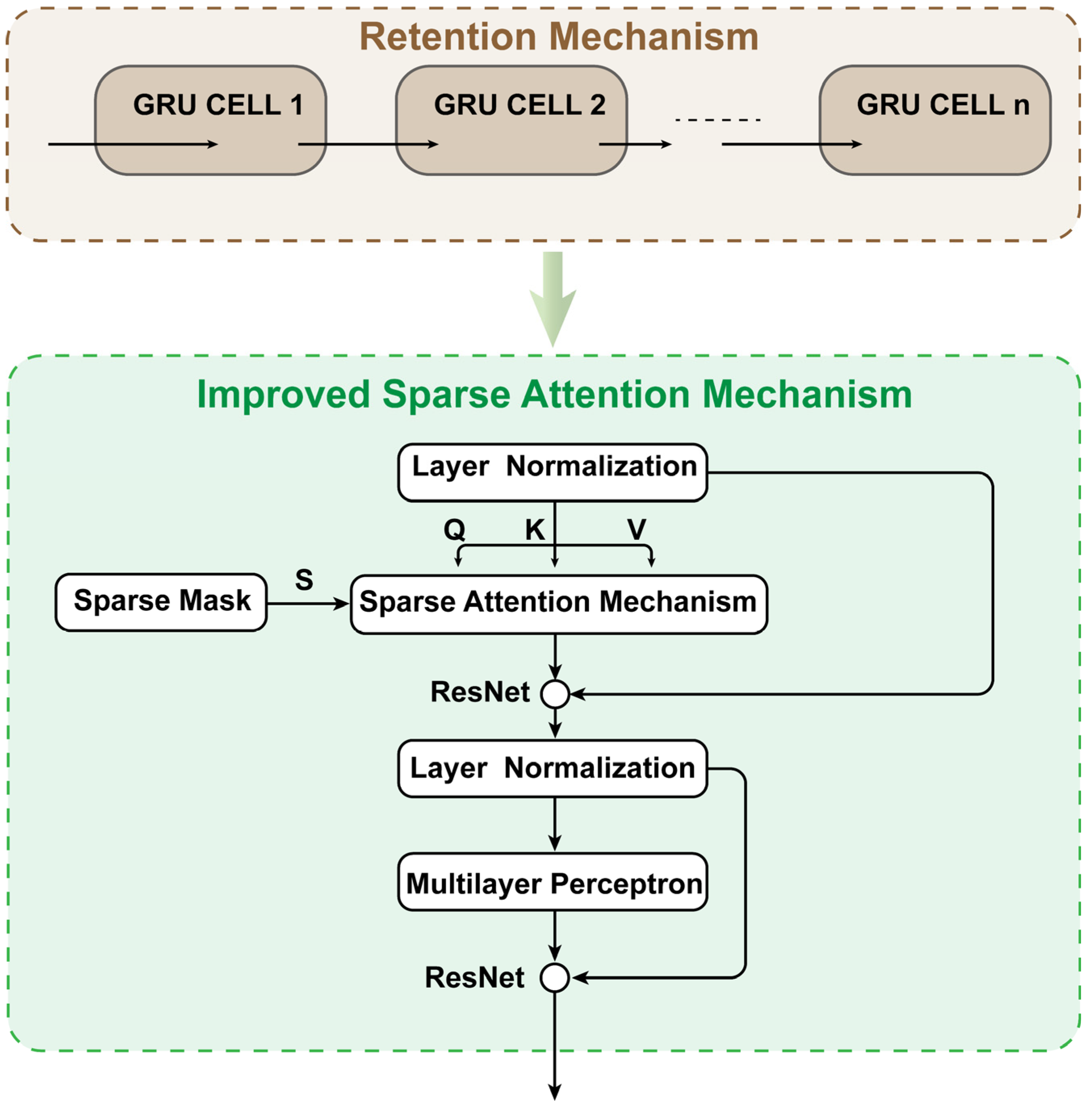
The core functionality of PartsNet is integrated within Encoder-Net, as shown in Figure 3. Encoder-Net takes the dimensionality-reduced data processed by GDR-Net as input, combining the attention and retention information from the sequence data to produce the output. The GRU layer yields a sequence matrix H comprising the hidden layer states, which serves as the initial extraction of the feature information from the sequential data. By introducing an improved sparse multi-head attention mechanism, weights are assigned to each hidden layer state of the sequence matrix. This addresses the issue of long-term dependencies in sequence data and reduces the time complexity of the Transformer multi-head attention from to
.

Figure 3.
The architecture diagram of Encoder-Net in PartsNet.
2.2.1. Gated Recurrent Unit (GRU) Layers
An RNN encounters two drawbacks when dealing with sequential data. Firstly, the limited retention capacity leads to the issues of vanishing or exploding gradients. Secondly, the model’s dependence on sequential data results in low parallelism. The GRU proposed by Cho et al. [36] in 2014 demonstrated good performance in sequential data prediction [8].
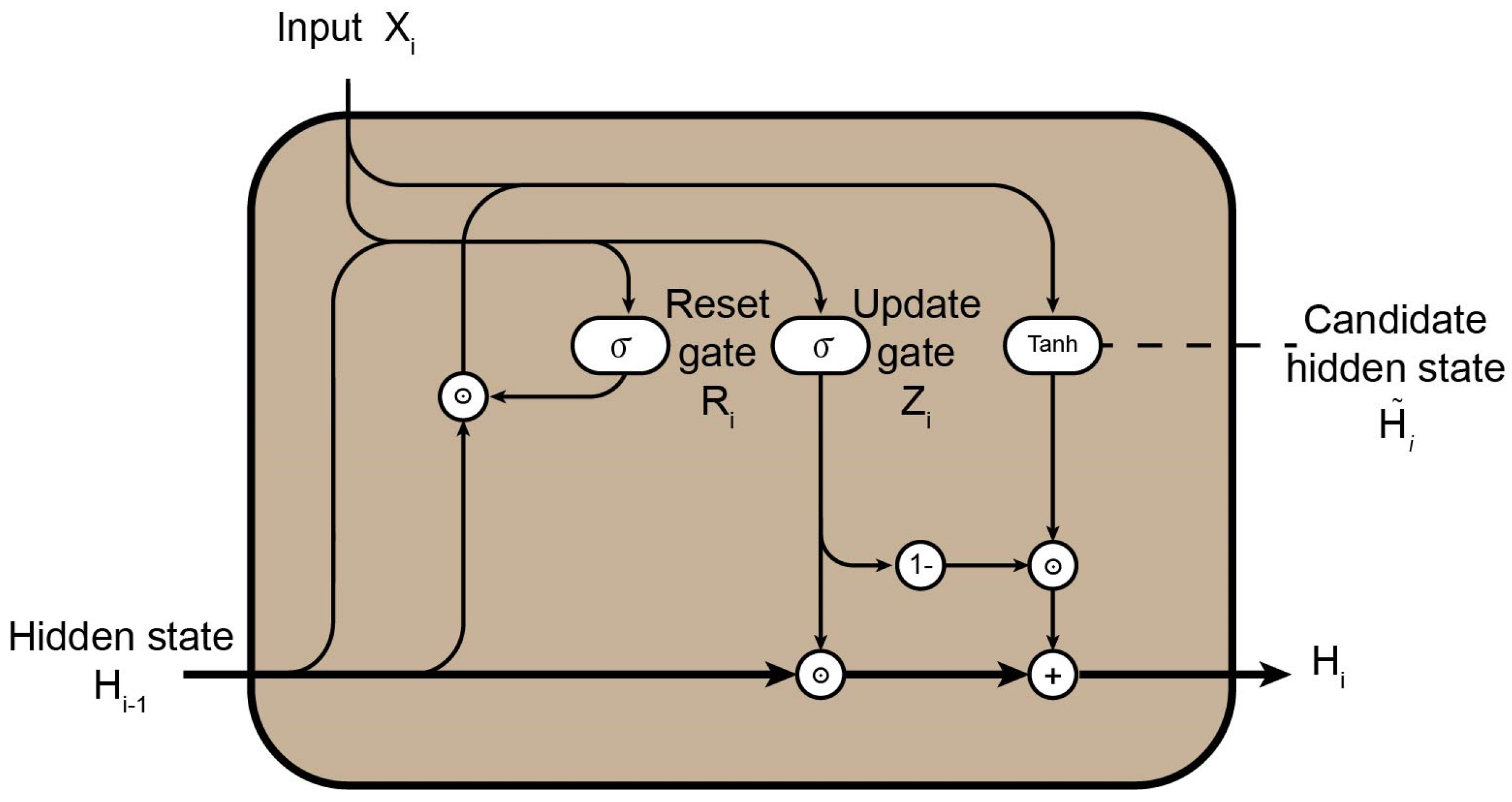
The GRU handles sequence data and learns the underlying structures through the reset gate and the update gate , as shown in Figure 4. represents the input data with sequence value of i, while denotes the hidden state vector output from the previous timestep of the GRU. Upon receiving inputs and , the current GRU computes the gate control states and through a calculation process.
is responsible for controlling to what extent the previous feature information can be remembered and how it should be incorporated into the candidate hidden state . filters out certain information from , retaining only the relevant and useful portions, enabling the neural network to exhibit retention capability.

Figure 4.
Schematic diagram of GRU module.
reflects the retention capacity of the GRU, while determines the strength of the retention. The GRU ultimately outputs the current hidden state vector, which is a weighted sum of and the current candidate hidden state .
Here, and are activation functions, and their output ranges are and , respectively. , , , , , and represent weight matrices, while , , and represent bias terms.
2.2.2. Improved Sparse Multi-Head Attention Mechanism
The Transformer [37] is a sequence-to-sequence model that utilizes the multi-head attention mechanism. The attention mechanism assigns different weights to the information from each timestep and compares it to the information from the current timestep in order to better capture implicit structures and long-range dependencies in sequence data. The self-attention mechanism can be represented by the following equation:
where Q, K, and V are obtained by linear transformations applied to the input sequence. represents the dimensionality of each query vector. represents the similarity matrix between the query and key vectors, and it corresponds to the inner product projection of the tensors.
Multi-head attention strengthens the ability of the neural network to capture highly nonlinear relationships. It consists of multiple independent self-attention layers, referred to as “heads.” Each head has its own set of learnable weight matrices, allowing it to capture different features and semantic information from the input sequence. The splitting of matrices is performed as follows: .
The multi-head attention mechanism is calculated as follows:
These transformation matrices belong to the vector space as follows: , , and . is a linear transformation matrix so that the dimensions of the input and output are the same. H represents the number of heads. The time complexity of the multi-head attention mechanism is , and n represents the length of the sequence.
This paper proposes a sparse multi-head attention mechanism based on a sparse mask, aiming to reduce the time complexity of the Transformer encoder while ensuring learning accuracy. A sparse mask matrix, which has the same shape as , is designed in this study. The dimensions to be preserved in the original projection matrix are determined based on the hyperparameter sparsity, which yields a sparse threshold. Subsequently, information positions in the sparse mask that are less than or equal to the threshold are set to negative infinity and mapped to , introducing sparsity into the attention scores.
The sparse multi-head attention mechanism involves sorting the attention scores, mask processing, and conventional matrix multiplication. The overall complexity is denoted as , where n represents the length of the sequence. The performance of the proposed mechanism will be further demonstrated in the ablation experiments conducted in Section 4.2.
The processed retention data from the GRU layer is first subjected to layer normalization, making sure that each feature dimension has a comparable mean and variance. After obtaining sparse attention weights, a residual connection [38] is used before the subsequent layer normalization for enhancing model robustness. Finally, a multilayer perceptron is used to further improve Encoder-Net’s nonlinear expressive capability.
2.3. Decoder-Net
Processing sequential data in the DEM differs logically from NLP tasks like machine translation. Sequential data do not require masks for information preservation due to their inherent continuity. The classic Transformer decoder is not suitable for the calibration task. Instead, the Decoder-Net of PartsNet incorporates a two-layer multilayer perceptron with residual connection. The size of the first layer is determined by the hidden size, while the second layer is contingent upon the number of calibrated parameters. Multilayer perceptron is capable of learning more complex nonlinear mapping relationships, while residual connection enhances gradient information stability. Through Decoder-Net, high-dimensional data are mapped to the low-dimensional space of the parameters to be calibrated. The decoder is calculated as follows:
Here, represents the activation function, represents the linear transformation based on multilayer perceptron, and x represents the input tensor in Decoder-Net. The output is a vector composed of parameters to be calibrated. The coordination of these neural networks realizes the “end-to-end” solution of parameter calibration.
2.4. Implementation Details
PartsNet was developed in this study using open-source frameworks such as PyTorch and NumPy. The training of PartsNet was conducted on a 12th Gen Intel(R) Core(TM) i5-12500H (Santa Clara, CA, USA). The hyperparameters used in the training process are summarized in Table 1. Two sets of hyperparameters were selected for the following two scenarios, respectively.

Table 1.
List of PartsNet hyperparameters.
3. Triaxial Compression Calibration Test and Verification
This section discusses the parameter calibration case of PartsNet, focusing on its application in calibrating the EEPA model and employing it to simulate the mechanical behavior of elastoplastic wet sand under triaxial compression.
3.1. Edinburgh Elasto-Plastic Adhesion Model (EEPA)
The interaction among a granular system like wet sand is highly complex, influenced by factors such as surface topography, chemical properties, and the characteristics of the interstitial medium [39]. The EEPA model is an extension of the linear viscoelastic model [40]. This model can effectively simulate the nonlinear force-displacement behavior during compression and incorporates both viscous damping and rolling resistance mechanisms, similar to a linear rolling resistance model. In this study, EEPA (Figure 5) is employed to describe the elastoplastic wet sand, and PartsNet calibrates the key parameters of EEPA.
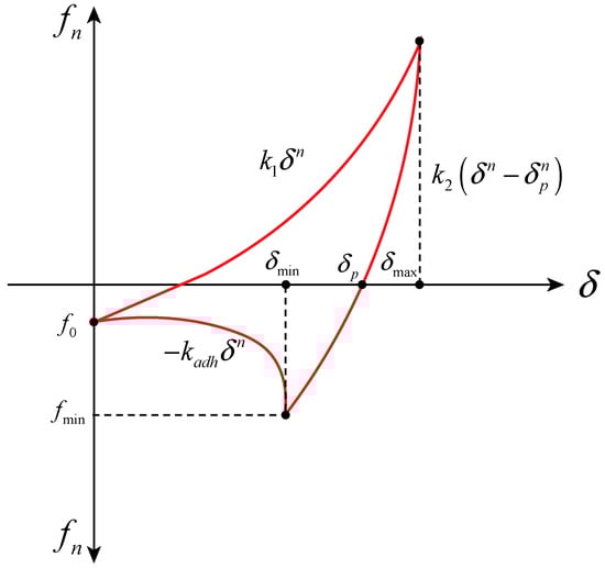
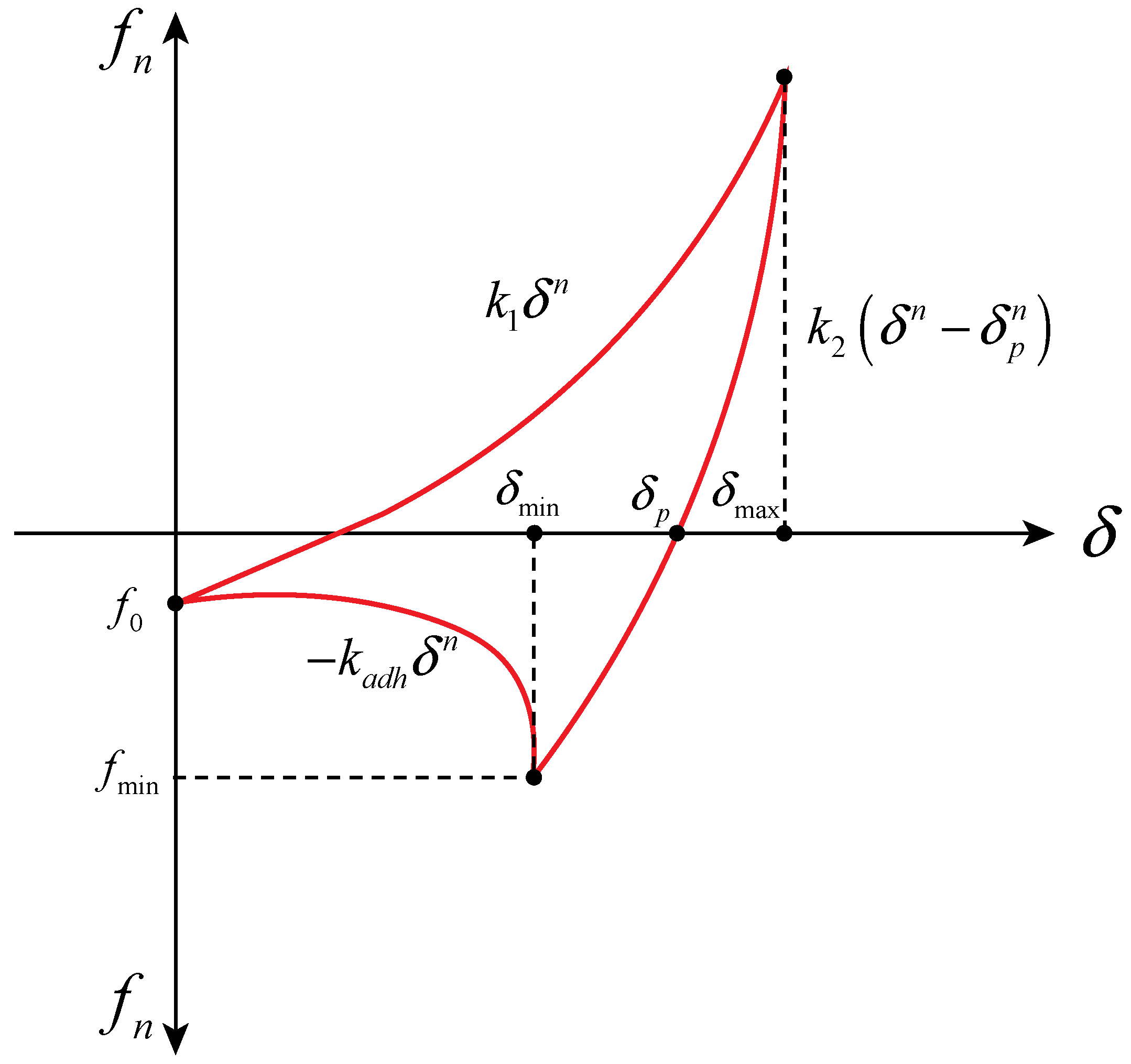
Figure 5.
EEPA normal loading–overlapping displacement diagram.
EEPA is influenced by seven parameters: the initial loading stiffness , unloading and reloading stiffness , contact plasticity ratio , constant pull-off force , adhesion energy parameter , stiffness exponent n, and adhesiveness exponent . The stiffness exponent n takes two values, 1 and 1.5, with indicating whether the model is equivalent to a linear elastic model. In order to define the nonlinear behavior during loading and unloading, this study adopts a value of 1.5 for n.
The overall normal force is composed of two parts, the hysteresis spring force and the normal damping force :
Here, is the unit normal vector pointing from the contact point towards the center of the particle. The mathematical expression for the normal hysteresis spring force can be represented as follows:
The normal damping force can be expressed as follows:
Here, represents the normal overlap, represents the normal plastic overlap, represents the adhesive stiffness, and represents the relative normal velocity generated during particle contact. is defined by the Hertzian contact theory, and its magnitude depends on the equivalent radius of particles, , and the equivalent Young’s modulus, , in the particle system.
is defined based on the ratio of two-stage stiffness, and a value of 0 indicates the elastic contact of particles.
represents the Hertz normal stiffness, which depends on the equivalent radius, Young’s modulus, and the normal overlap quantity .
represents the normal damping coefficient of the nonlinear model, and its calculation formula is provided by Morrissey [31].
Similarly, the total tangential force is also the sum of the tangential spring force and the tangential damping force :
where is the unit vector pointing tangentially from the contact point to the center of the particle, and is defined in incremental form (for the nth time step):
Here, , is the tangential stiffness, and is the tangential overlap.
is the tangential stiffness multiplier, and in this paper, . represents the equivalent shear modulus. The critical force for tangential force coupling with normal force can be determined based on the Coulomb friction criterion:
Here, represents the maximum tangential friction force, and is the friction coefficient. The modeling theory of EEPA can also refer to [8,13,39,41].
3.2. Test and Numerical Simulation of Triaxial Compression in Wet Sand
3.2.1. Triaxial Compression Test in Wet Sand
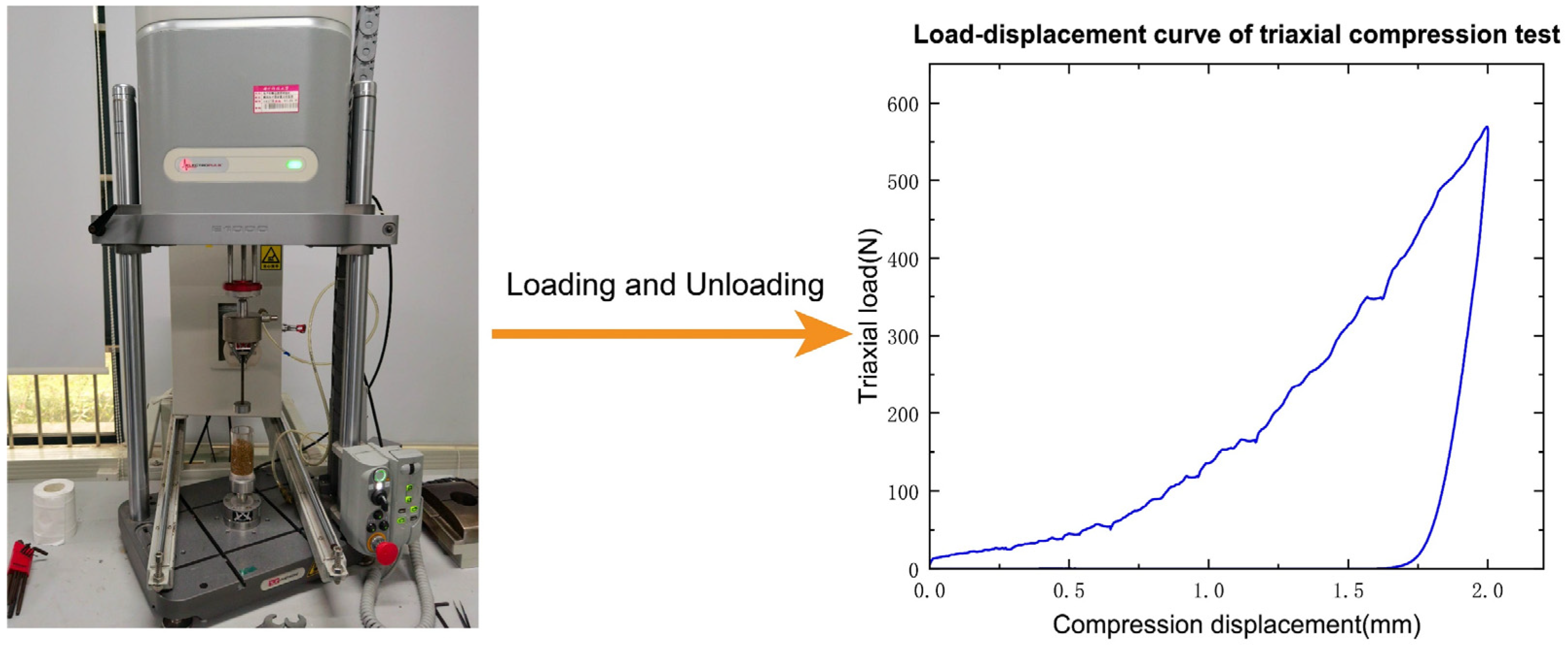
A triaxial test was conducted using the electronic dynamic–static fatigue testing machine at the Huazhong University of Science and Technology, as illustrated in Figure 6. The experimental material chosen consisted of wet sand characterized by particle sizes ranging from 1 mm to 2 mm with an aggregate weight of 80 g. The moisture content of the sand was measured to be 6.98%, with a pH value of 7.2. The moisture content is used to characterize the aggregation of the system. The density of the sand was measured before the experiment and found to be 2 g/cm3. The samples were loaded into acrylic cylinders with an outer diameter of 45 mm, an inner diameter of 35 mm, and a height of 85 mm, with a loading height of 60 mm. The loading and unloading speeds during the experiment were set to 0.5 mm/s and 0.2 mm/s, respectively. The data were sampled at a frequency of 200 Hz, and the load threshold of the testing machine was set to 600 N. Based on the experimental results, it was observed that the sand exhibited significant differences in stiffness between loading and unloading, with the nonlinear behavior being more pronounced during the loading phase.
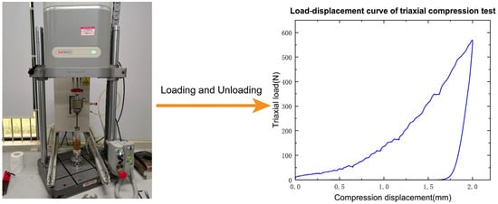
Figure 6.
Sand triaxial compression test and its “load–displacement” curve.
3.2.2. Simulation of Triaxial Compression by DEM
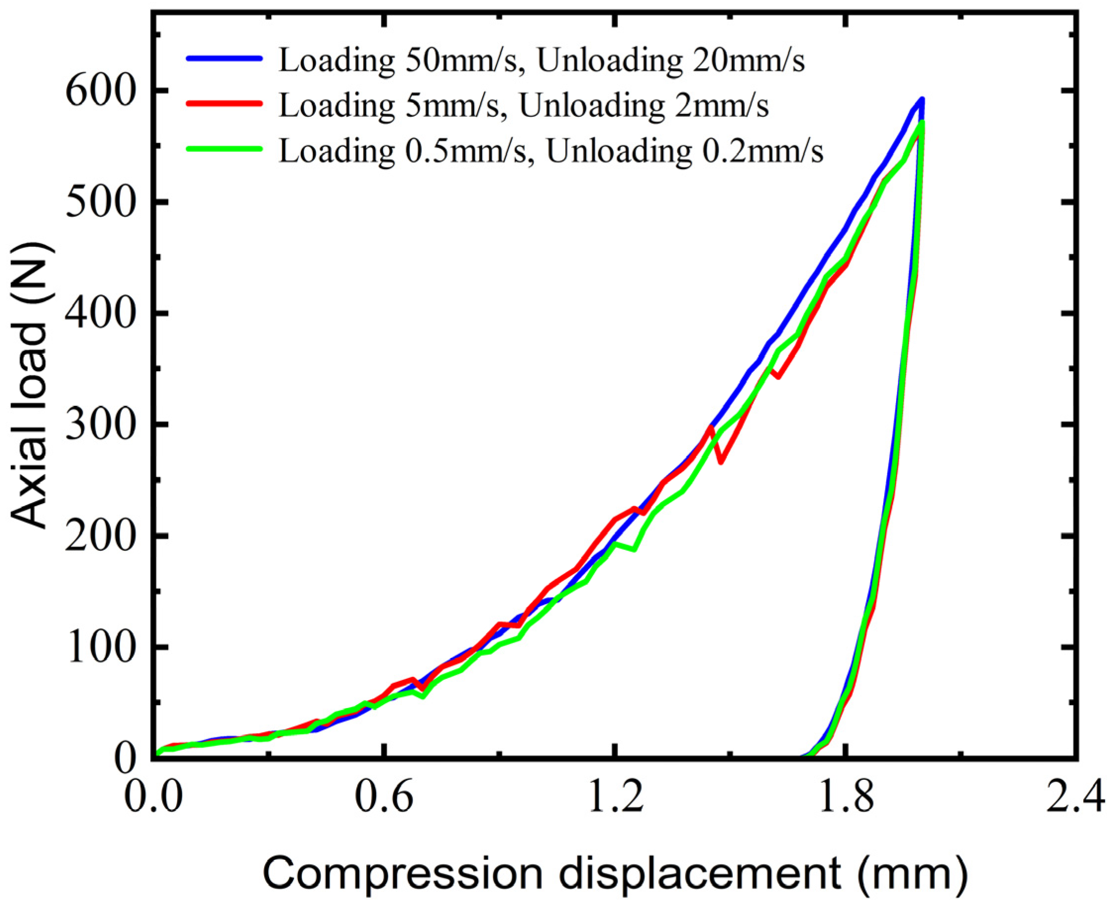
In discrete element studies, using spherical particles to represent sand is common [42,43]. A total of 8238 particle units were generated, and a simulation model was established based on the experimental conditions. To ensure uniform force distribution in the granular system during simulation, a small load was applied for pre-compression and allowed to settle until the longitudinal force reached a stable value of 1.82 N. The process of loading and unloading through the piston is the critical stage in the DEM simulation. Due to the computational complexity of the DEM, it would be time-consuming to perform the simulation directly using the experimental loading and unloading velocities. To address this, a sensitivity analysis based on varying velocity gradients was performed to assess the dynamic response of wet sand to loading and unloading velocities. The sensitivity analysis results, depicted in Figure 7, include three experimental setups. The first setup utilized a loading speed of 50 mm/s for 0.04 s and an unloading speed of 20 mm/s from 0.04 to 0.06 s. The second setup featured a loading speed of 5 mm/s for 0.4 s and an unloading speed of 2 mm/s from 0.4 to 0.6 s. The third setup mirrored the actual experimental conditions with a loading speed of 0.5 mm/s for 4 s and an unloading speed of 0.2 mm/s from 4 to 6 s. The simulation times for these setups were 0.1714 h, 1.2985 h, and 6.467 h, respectively, with a notable increase in the computational time as the loading rate decreased. Despite the significant differences in the loading and unloading velocities, the load–displacement curves across all three setups exhibited similar nonlinear behavior with minimal variation. Consequently, to optimize simulation efficiency and enable the generation of a dataset through multiple simulation iterations, this study employed the loading and unloading velocities from the first setup for subsequent investigations. The other simulation conditions were consistent with the triaxial compression test. To accurately capture the data characteristics, we chose the sampling frequency as 2000 Hz, and each sequence of data was sampled 99 times. The entire simulation process is illustrated in Figure 8.

Figure 7.
Sensitivity analysis of load–displacement curve of discrete element triaxial compression test on loading and unloading velocities.
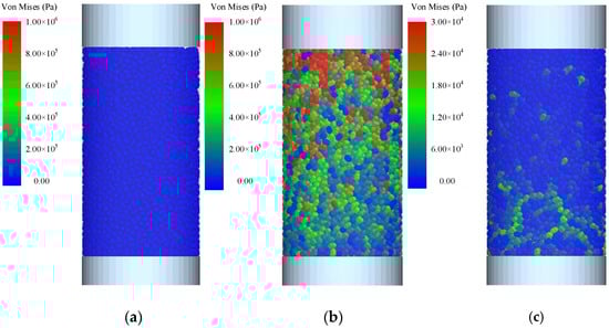
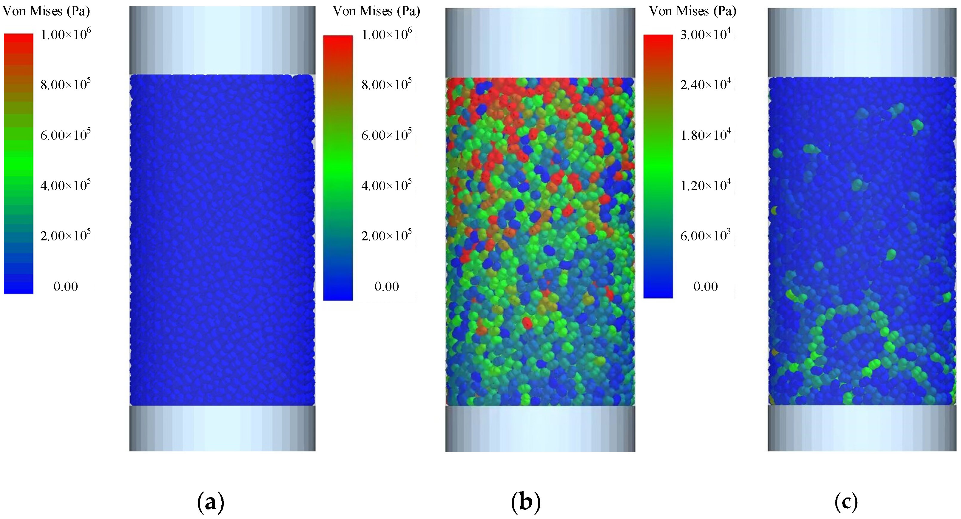
Figure 8.
An overall simulation diagram of the triaxial compression test based on EDEM 2022. (a) At the infancy of the experiment, the wet sand is subjected to uniform forces after the preloading treatment. (b) As the loading progresses, the upper part of the wet sand experiences higher stresses, and the stress is gradually propagated along the force chains in the longitudinal direction. (c) After the unloading process is completed, the system retains residual stresses, exhibiting certain plastic behavior, which complies with the fundamental constraints of the EEPA model.
The DEM dynamics simulations in this research employ particles shaped as a dual sphere in EDEM 2022, where both spheres have a physical radius of 1 mm and are connected together by a contact zone. In the world coordinate system, the coordinates of these two spheres’ centers are, respectively, (−0.405 mm, 0.000 mm, 0.000 mm) and (0.405 mm, 0.000 mm, 0.000 mm). The smoothing value of the particles was set to 5. In order to accurately simulate the triaxial compression experiment, a container made of Perspex was used to simulate the acrylic tube in the experiment, and the upper surface of the wet sand was loaded and unloaded using a steel piston.
The experiment was simulated in EDEM 2022, and the input parameters used are shown in Table 2.
Table 2.
Simulation parameters of discrete element triaxial compression test.
In the dimensionality reduction experiment in Section 3.3, we found that , , and are significant parameters for EEPA. Accurately capturing these information-rich parameters enables neural networks to analyze the mechanical behaviors of macroscopic systems at a faster pace and with greater simplification, underscoring the significance of parameter calibration. Therefore, this paper expands the range of these three parameters and generates 200 sets of random numbers. These numbers are then used in EDEM 2022 to obtain 200 sets of simulation “load-displacement” sequence data for PartsNet training.
3.3. Training and Results of PartsNet
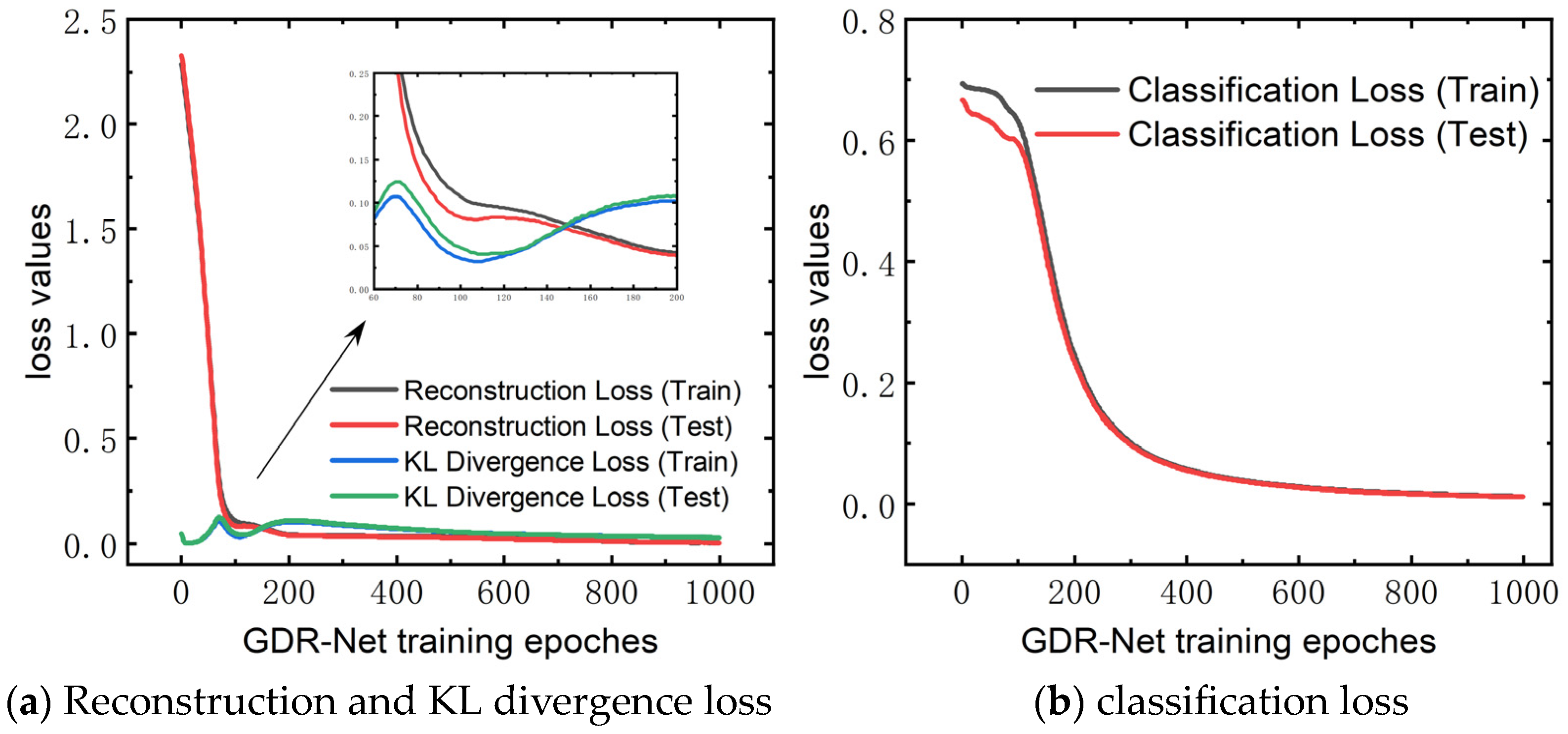
This section presents the calibration results and performance of PartsNet in the aforementioned case study. In the data preprocessing of triaxial compression, GDR-Net examined the significant preset parameters of EEPA and the main contact parameters of wet sand (). Through GDR-Net, feature dimension reduction and extraction were performed, resulting in three key parameters in the latent space. Figure 9 displays the loss results of GDR-Net. Reconstruction loss and KL divergence loss on the test set converged to 4.34 × 10⁻³ and 2.723 × 10⁻², respectively, while the classification loss converged to 1.235 × 10⁻². According to the principal component ordering, the relative weights of were found to be 0.378, 0.407, and 0.215, respectively. Therefore, had the most significant impact on the experimental results, followed by and .
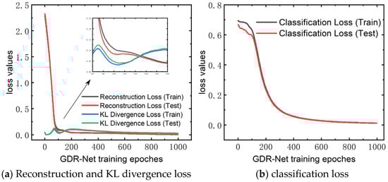
Figure 9.
Loss function results of GDR-Net dimensionality reduction for triaxial test.
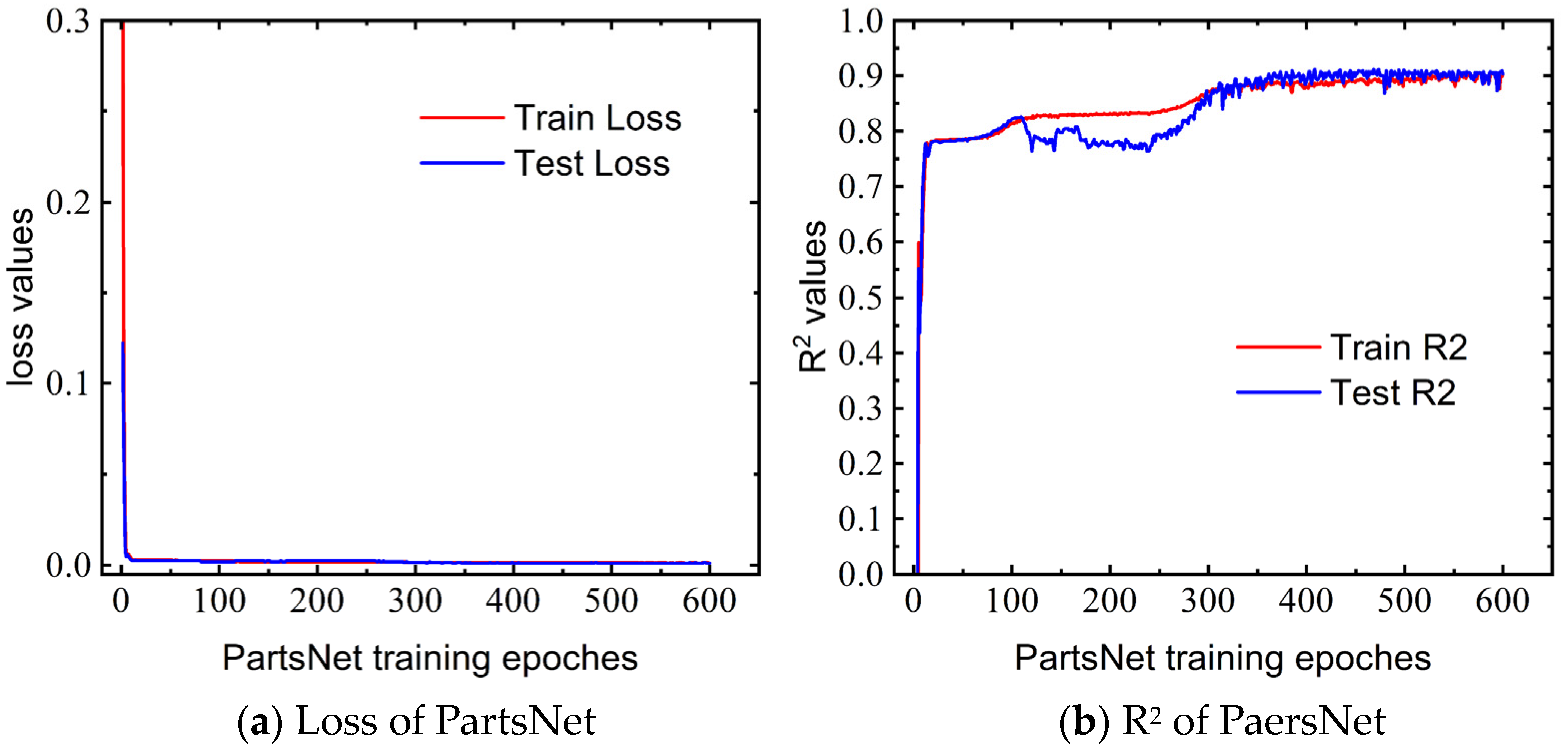
We conducted 200 sets of EDEM 2022 simulations, generating “load–displacement” curve data, which we subsequently utilized as an input dataset for PartsNet. Using the predicted parameters from PartsNet, simulations were performed, and the calibrated curve showed a good fit with the experimentally determined curve. Figure 10 illustrates the convergence of the MSE loss and coefficient of determination (R2) during the training process. Parameter calibration can be seen as a regression prediction task, and using accuracy as an evaluation metric, as in classification problems, is not appropriate. Therefore, R2 was used as the criterion for accuracy. In the DEM dataset used in this study, PartsNet achieved MSE convergence at 9.34 × 10⁻⁴ and R2 convergence at 0.913.
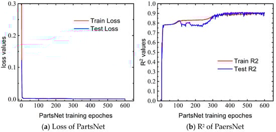
Figure 10.
Convergence results of PartsNet MSE loss and R2 for triaxial test.
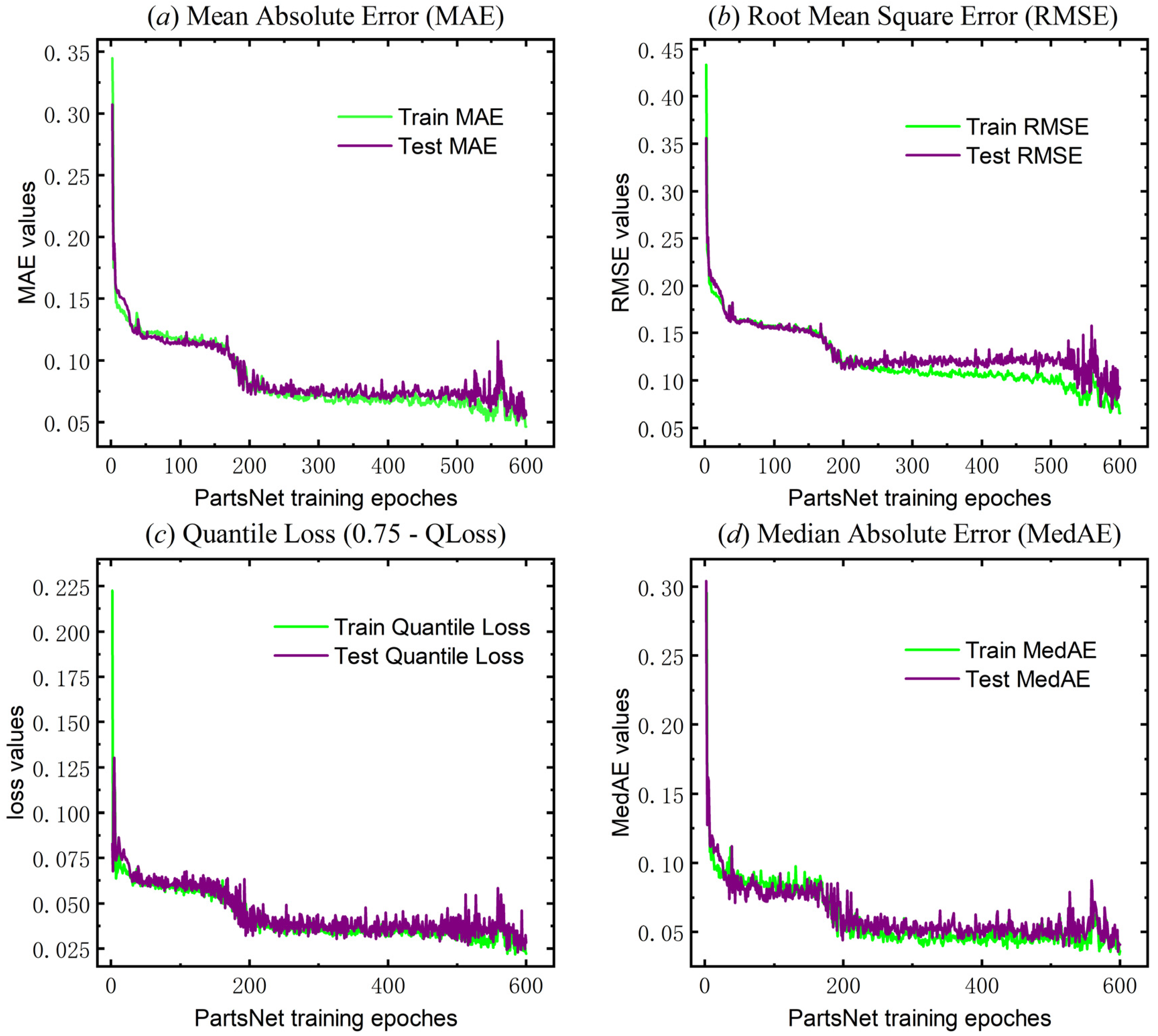
PartsNet incorporates additional, more thorough regression analysis evaluation metrics in addition to the fundamental evaluation metrics (loss functions and coefficient of determination) to describe the calibration performance. The specific calculation formulas can be found in Appendix A. Figure 11 illustrates the convergence of additional evaluation metrics, including the Mean Absolute Error (MAE), Root Mean Square Error (RMSE), Median Absolute Error (MedAE), and the 0.75-quantile loss (0.75-QLoss) when Q = 0.75 during the training process of PartsNet. They converge at 0.019, 0.031, 0.011, and 0.008, respectively. Furthermore, it is worth noting that the training time of PartsNet is only 159.586 s, which will be further analyzed for its significant advantage in the ablation experiment in Section 4.2.
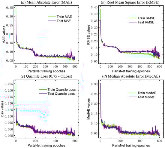
Figure 11.
Other evaluation indexes of Part-Net for triaxial test (MAE, RMSE, 0.75-QLoss, and MedAE).
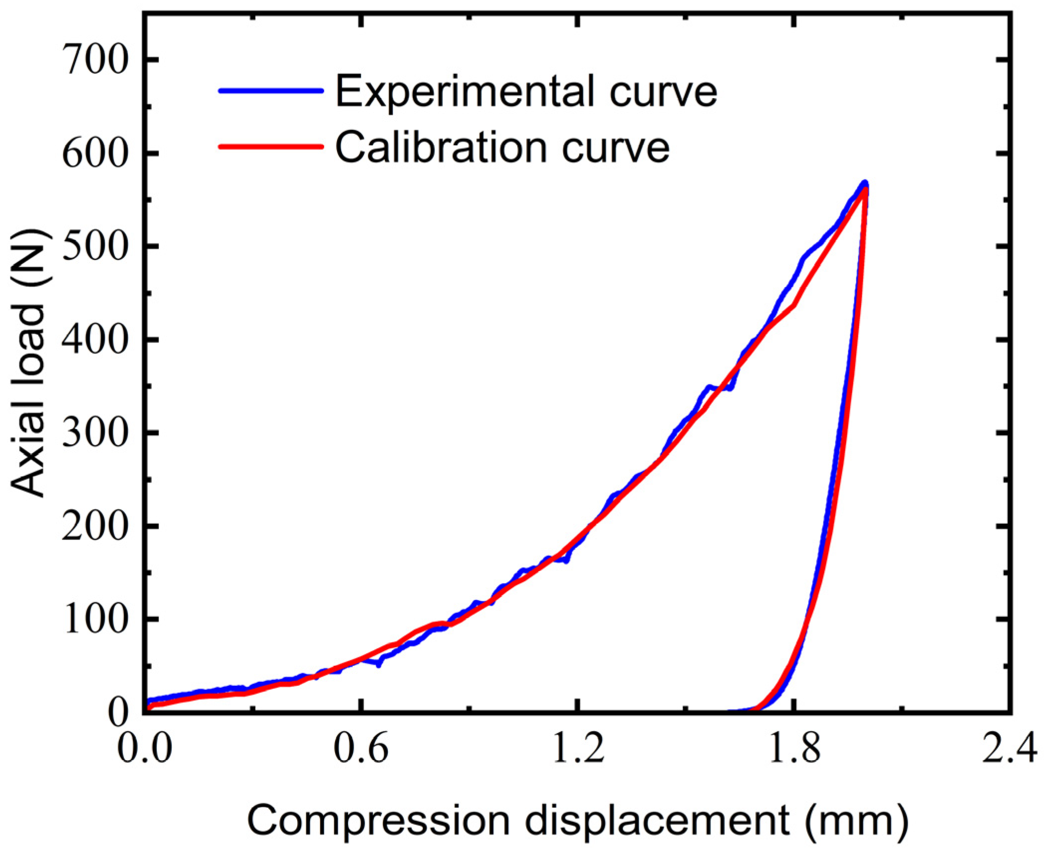
The neural network trained using the aforementioned process can be used to predict the key simulation parameters of the triaxial compression calibration test:. Figure 12 illustrates the comparison between the simulated sequence data generated using the calibrated parameters and the experimental data. The nonlinear behaviors are well captured, and the calibrated curve reflects the visco-plastic coupling behavior of EEPA. During the initial loading phase, the changing rate in the slope of the calibration curve closely mirrors that of the experimental data, and it accurately predicts both the trends in load and displacement peaks. Moreover, it provides a highly precise description of the unloading phase and residual stress.

Figure 12.
Comparison between parameter calibration curve and triaxial test curve.
PartsNet enhances the fidelity of DEM simulations pertaining to the triaxial compression of elastoplastic wet sand by incorporating time series response data. Through the calibration of key parameters of the EEPA constitutive model, the calibrated model accurately captures the nonlinear sequential mechanical behavior within elastoplastic wet sand. Consequently, PartsNet elevates the precision of DEM simulations concerning loading conditions in elastoplastic wet sand. This method demonstrates excellent capabilities in elastoplastic mechanics calibration tasks. With this method, the issue of unidentifiability in constitutive parameters and their combinations in DEM can be addressed. PartsNet can also be generalized to other scenarios involving multiple processes and coupled physical fields. By directly associating the sequential input data with the key parameters, PartsNet provides a unified solution for parameter calibration that integrates attention and retention.
3.4. Verification Tests for PartsNet
After the confirmation of PartsNet for its accuracy, more intricate cases will be calibrated to demonstrate its general applicability in calibrating the EEPA constitutive relationship for elastoplastic wet sand. In practice, these force–displacement sequential data can be obtained from the above experimental instruments, while here, for simplicity, this paper uses the DEM simulated data generated by the DEM as ground truth. Nine sets of parameter combinations , were sampled based on the Gaussian distribution, deliberately including design points beyond the scope of the original training dataset of PartsNet. Numerical experiments were conducted using EDEM 2022. Experimental data were then predicted using the pre-trained PartsNet to calibrate the corresponding parameters. The relative errors between the calibrated parameters and the true parameters are displayed in Table 3.
Table 3.
The actual parameters and calibration parameters of 9 verification cases.
Excellent accuracy is achieved by PartsNet in the prediction of parameters and , with the majority of relative errors for , which is the most weighted, being within 1%. Parameter , with a smaller weight and sharing some out-of-training-set design points with , has relative errors exceeding 10% in three cases.
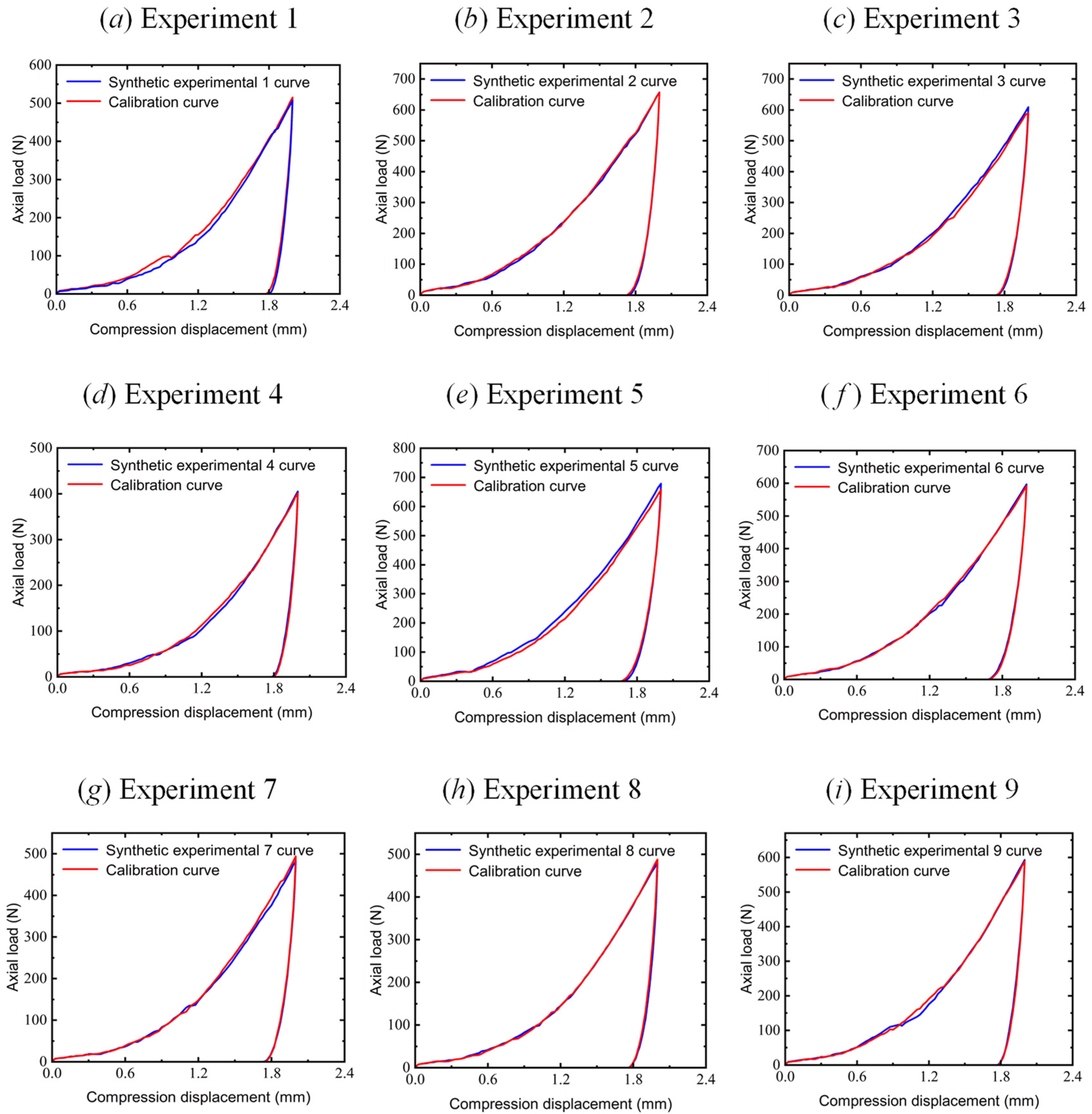
Figure 13 illustrates the calibration results of PartsNet for the nine validation experimental datasets and compares them with the experimental force–displacement curves. The parameters calibrated by PartsNet accurately capture the EEPA constitutive relationship during the loading and unloading processes of the elastoplastic wet sand. The dynamic response obtained from EDEM 2022 exhibits good consistency with the experimental curves, reflecting the dynamic trends, peak load values, and post-unloading displacement values.
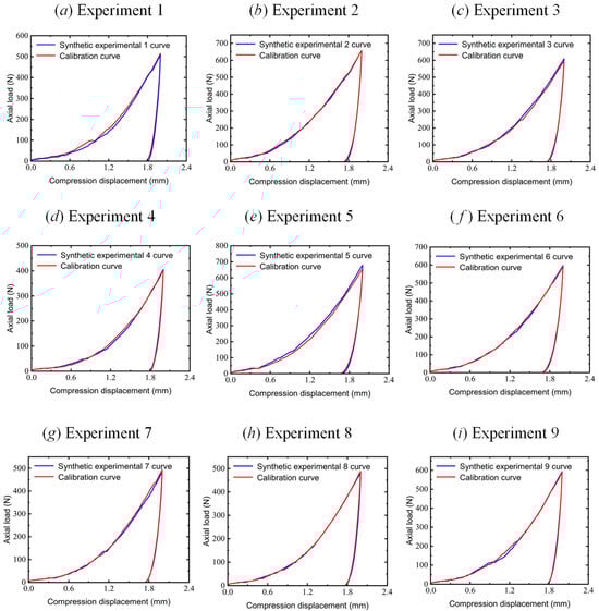
Figure 13.
Comparison of parameter calibration curves and triaxial test curves in 9 groups of verification experiments.
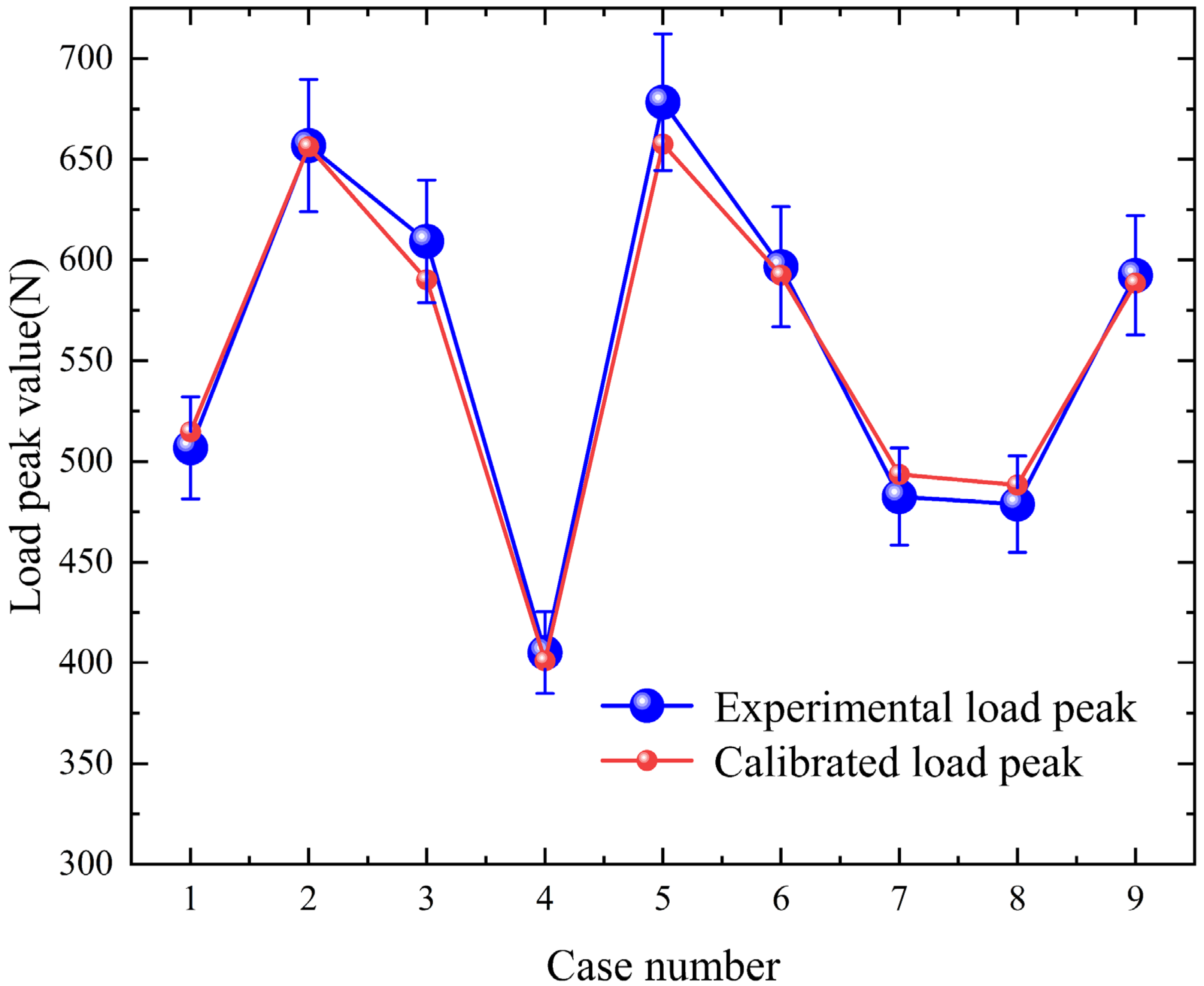
The peak load values from the nine validation experiments are discretely distributed between 405.138 N and 678.339 N. In Figure 14, 5% of the experimental peak load is used as error bars to assess the calibration of peak load values. It was found that the results from PartsNet accurately match the experimental data, all falling within the confidence interval. This indicates that PartsNet maintains accuracy even under extreme conditions.
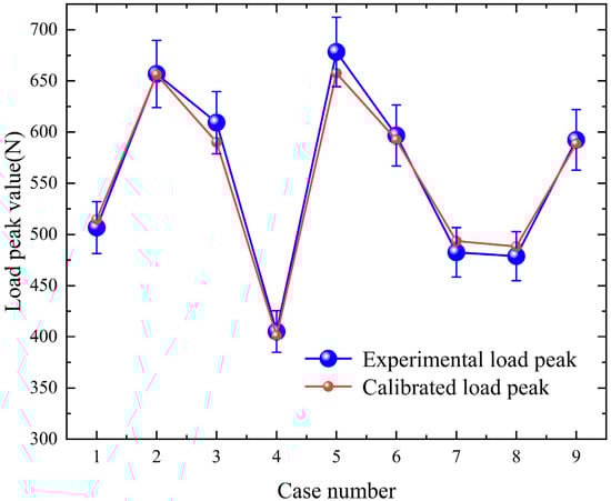
Figure 14.
Comparison of calibrated load peaks and experimental load peaks in 9 groups of verification experiments.
The most precise peak fit and the least amount of error are found in the ninth dataset. These parameters, , fs−s, fs−a, determine the micromechanical behavior and macroscopic response of the sand. The simulation stress–strain curve is faithfully reproduced when the contact plasticity ratio is chosen accurately, capturing the subtleties of the material’s elastic–plastic transition during contact. The accuracy of the static friction coefficient between particles fs−s directly affects the prediction of the shear strength and the formation and evolution of the shear zone, which realistically reproduces the sliding and rolling behaviors between particles. The distribution of wall shear stress and particle flow resistance may be accurately simulated by the static friction coefficient between the sand and the wall fs−a. This, in turn, influences the sand’s total deformation and energy dissipation.
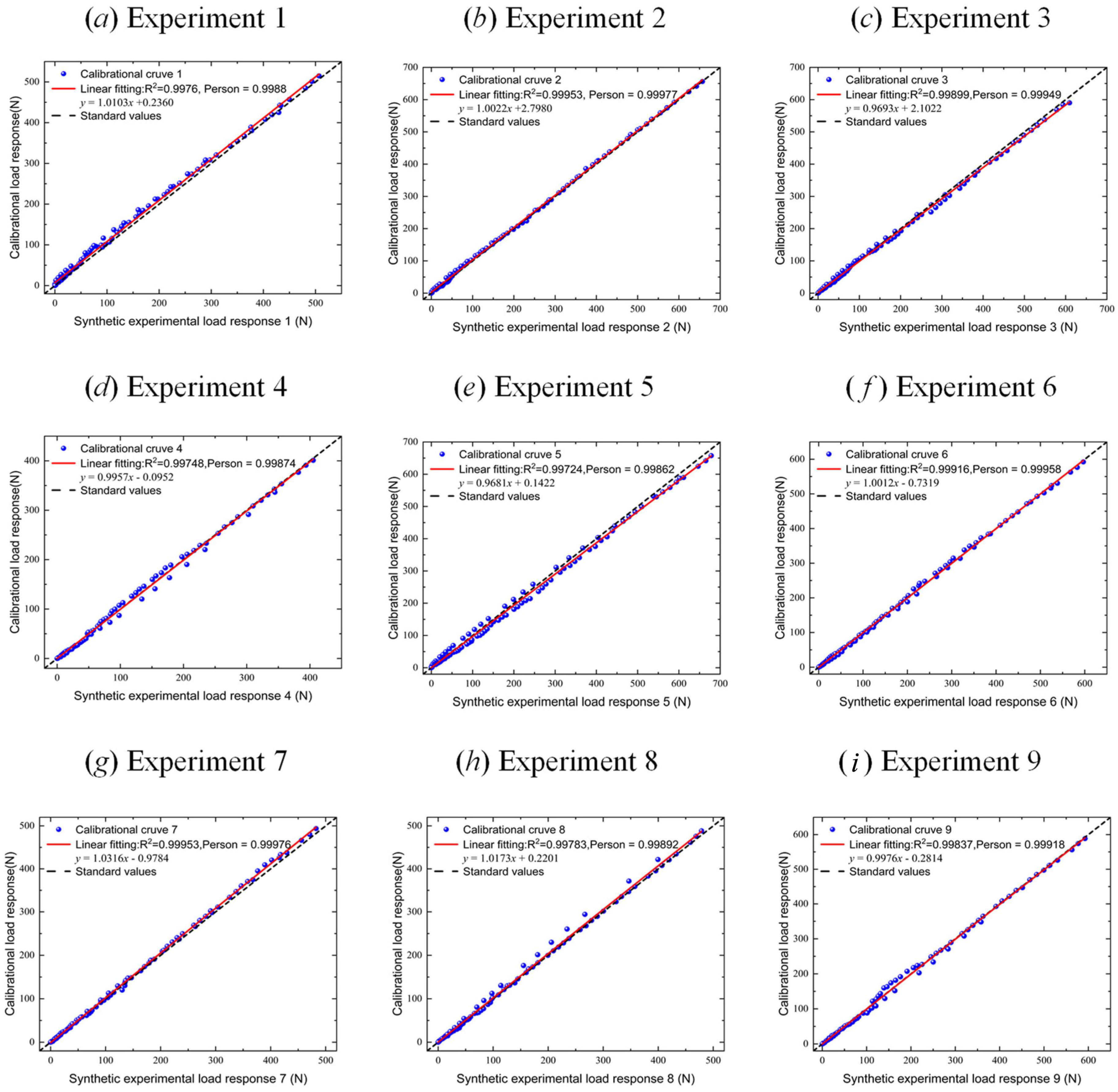
Figure 15 depicts the correlation assessment between the dynamic responses obtained using calibrated parameters and test data across nine validation experiments. This assessment includes R2 values, Pearson correlation coefficients, and linear fitting results. All cases exhibit R2 values and Pearson correlation coefficients exceeding 0.99. The fitting coefficients range between 0.968 and 1.032, highlighting remarkable calibration accuracy. Through these nine numerical experiments, the generalization capacity of the PartsNet capacity is validated, providing reasonable inferences for assumption space distributions located at the periphery of the pre-trained dataset.
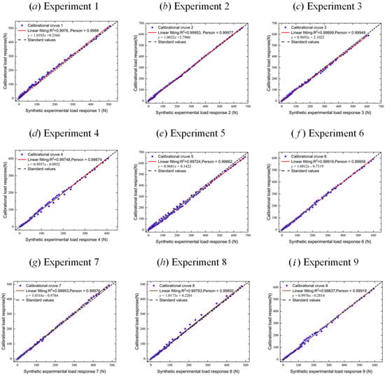
Figure 15.
Comparison of linear fitting results between calibrated load responses and test load responses in 9 groups of verification experiments.
4. Discussions
4.1. Ablation Test and Calibration Performance Analysis
To demonstrate the outstanding calibration performance of PartsNet in addressing the issue of parameter unidentifiability, we designed the following four sets of ablation experiments: pure RNN and GRU, RNN and GRU with dot-product attention mechanism, RNN and GRU with Transformer encoder (TransE), and RNN and GRU with our proposed sparse mask-based sparse attention mechanism Transformer encoder (STE). The comparison between the first set and the other sets highlights the necessity of introducing the attention mechanism, while the comparisons within the latter three sets reveal the differences among the different types of attention mechanisms in the DEM parameter calibration task. PartsNet demonstrates state-of-the-art performance in these experiments based on multiple indexes.
Table 4 presents the ablation experiments conducted on PartsNet and other neural networks. In these experiments, the eight networks shared the hyperparameters specified in Section 2.4. Across all evaluation metrics, RNNs without attention mechanisms performed the worst, with a nearly 40% lower calibration accuracy compared to PartsNet. The introduction of dot-product attention led to some improvements. It is crucial to emphasize that PartsNet achieves the highest training accuracy (0.913) while simultaneously attaining a decent convergence speed. Specifically, PartsNet exhibits an improvement with a speed advantage of 21.25% over the Transformer encoder–GRU-based network. Additionally, the GRU performs significantly better than the RNN both with and without the addition of the attention mechanism. Overall, PartsNet demonstrated the highest calibration precision in these tasks and exhibited a significant advantage in terms of time compared to the multi-head attention mechanism used in Transformer.
Table 4.
Ablation experimental data of PartsNet in triaxial test.
4.2. Error Quantization Format of PartsNet
Error analysis is a crucial component in quantitatively describing the accuracy of numerical computations. In this study, we proposed the error quantification format for parameter calibration. Errors can be broadly categorized into systematic errors and random errors. Systematic errors can be understood as the limited expressive power of numerical models and the constrained optimization ability of algorithms, including deep learning. Random errors arise from the varying degrees of numerical discrepancies observed in experiments and calculations.
Here,
Indeed, the analysis of random errors in mechanical engineering can be complex. Common sources of such errors include limitations in sensor accuracy and unavoidable environmental noise, leading to measurement errors. In this study, we currently do not focus on quantifying these errors stemming from inherent priors. Instead, our main emphasis is on quantifying systematic errors.
Systematic error is primarily composed of , which originates from the constitutive relationship of the model. The quantitative constitutive relationship serves as a dimensional reduction representation of the real system, and the information lost during this process contributes to the error. Systematic error represents the upper limit of all objective limitations of the parameter calibration algorithm. Without loss of generality, this study employs a third-order Taylor expansion to calculate and utilizes data-oriented numerical differentiation methods to compute gradients. The novelty of this approach lies in circumventing the issue of dimension reduction caused by deterministic constitutive relationships.
Let be an m-dimensional orthogonal sequence with N samples. We input this sequence into the trained PartsNet and use the predicted parameters to perform a simulation, resulting in another set of sequence data with the same shape.
The “order” parameter was set to 3 in this paper, and represents the expansion position, which we set to 10−7. This study introduces an adaptive difference algorithm to calculate the numerical derivatives of the discrete sequence. At each internal data point, the algorithm selects the smallest spacing as the step size based on the distances between neighboring data points and uses the central difference scheme to compute the derivative value. For boundary points, forward and backward difference schemes are still used. This method adjusts the step size based on the local characteristics of the data points, improving the accuracy and stability of numerical differentiation.
The optimization of the system error reflects the accuracy of the optimization algorithm in parameter calibration, which is also a demonstration of the superiority of deep learning. In PartsNet, the MSE is employed to quantify the system error.
Here, represents the mapping relationship learned by PartsNet, and represent the corresponding label values.
We fully defined and quantified the systematic error. The results of the ablation experiments demonstrate that PartsNet and the GRU architecture based on the Transformer encoder outperform other networks in terms of calibration accuracy. Therefore, we focus on analyzing the errors of these two network architectures in Table 5. In the triaxial test, the standard error of PartsNet is only one-fourth of that of the other method, indicating its significantly superior accuracy. This comparative experiment demonstrates the outstanding generalization of PartsNet from the perspective of error analysis.
Table 5.
Error quantization data for PartsNet and GRU with Transformer encoder.
5. Conclusions
This paper focuses on parameter calibration in the DEM and explores a universal parameter calibration method based on deep learning. We improve upon the multi-head attention mechanism by proposing a sparse multi-head attention mechanism implemented using a sparse mask matrix. This paper also establishes an error quantification format for parameter calibration. By utilizing the Taylor expansion form of the difference function, an adaptive differencing method is introduced to establish a quantitative analysis of errors in discrete sequences. PartsNet is an innovative end-to-end solution, which efficiently calibrates constitutive parameters by integrating attention and retention mechanisms. The conclusions of this study mainly reveal two aspects:
- The attention retention fusion with the deep learning mechanism, PartsNet, addresses long-term dependencies in calibrating parameters using high-dimension sequential dynamical information on wet sand. The microscale parameters calibrated through PartsNet excellently describe the macroscopic mechanical behavior and nonlinear mechanical properties of elastoplastic wet sand, surpassing the results achieved by existing methods. The performance of PartsNet in wet sand within the triaxial compression test and its verification tests highlight its robust generalization capacity.
- PartsNet demonstrates the capability to accurately obtain the EEPA model’s constitutive parameters of elastoplastic wet sand, surpassing seven other deep learning approaches in the ablation test. In the triaxial compression calibration test, PartsNet demonstrates the best predictive accuracy (91.29%) and surpasses the Transformer encoder–GRU architecture by 1.12% while achieving a 21.25% faster convergence. Moreover, the standard error of PartsNet is only one-fourth of that of the other method.
Author Contributions
Conceptualization, Z.H. and X.W.; Methodology, Z.H. and X.W.; Software, Z.H., X.Z., S.B. and Z.Z.; Validation, Z.H., J.Z., Z.Z. and X.W.; Formal analysis, Z.H., J.Z., Z.Z. and X.W.; Investigation, Z.H., J.Z., S.B., Z.Z. and X.W.; Resources, Z.Z. and X.W.; Data curation, Z.H., X.Z. and S.B.; Writing—original draft, Z.H., S.B. and X.W.; Writing—review & editing, Z.H., J.Z., Z.Z. and X.W.; Visualization, Z.H., X.Z., S.B. and Z.Z.; Supervision, X.W.; Project administration, X.W. All authors have read and agreed to the published version of the manuscript.
Funding
This research received no external funding.
Institutional Review Board Statement
Not applicable.
Informed Consent Statement
Not applicable.
Data Availability Statement
The raw data supporting the conclusions of this article will be made available by the authors on request.
Conflicts of Interest
The authors declare no conflict of interest.
Appendix A
Appendix A.1. Mathematical Definitions of Evaluation Index for PartsNet
Apart from the Mean Squared Error (MSE) loss function mentioned in the manuscript, PartsNet also supports the use of the following evaluation metrics to quantify the learning performance of this regression prediction problem.
Appendix A.2. Mean Absolute Error (MAE)
Appendix A.3. Root Mean Squared Error (RMSE)
Appendix A.4. Coefficient of Determination (R2)
Appendix A.5. Median Absolute Error (MedAE)
Appendix A.6. Quantile Loss Function (QLoss)
Here, or represents the mapping relationship learned by PartsNet, and represents the corresponding label values.
References
- Sun, W.; Sun, Y.; Wang, Y.; He, H. Calibration and experimental verification of discrete element parameters for modelling feed pelleting. Biosyst. Eng. 2024, 237, 182–195. [Google Scholar] [CrossRef]
- Colaprete, A.; Toon, O.B. Carbon dioxide snow storms during the polar night on Mars. J. Geophys. Res. Planets 2002, 107, 5-1–5-16. [Google Scholar] [CrossRef]
- Vo, T.T.; Nezamabadi, S.; Mutabaruka, P.; Delenne, J.Y.; Radjai, F. Additive rheology of complex granular flows. Nat. Commun. 2020, 11, 1476. [Google Scholar] [CrossRef] [PubMed]
- Shaghaghi, T.; Ghadrdan, M.; Tolooiyan, A. Effect of rock mass permeability and rock fracture leak-off coefficient on the pore water pressure distribution in a fractured slope. Simul. Model. Pract. Theory 2020, 105, 102167. [Google Scholar] [CrossRef]
- Ding, X.; Wang, B.; He, Z.; Shi, Y.; Li, K.; Cui, Y.; Yang, Q. Fast and precise DEM parameter calibration for Cucurbita ficifolia seeds. Biosyst. Eng. 2023, 236, 258–276. [Google Scholar] [CrossRef]
- Shi, Q.; Wang, B.; Mao, H.; Liu, Y. Calibration and measurement of micrometre-scale pollen particles for discrete element method parameters based on the Johnson-Kendal-Roberts model. Biosyst. Eng. 2024, 237, 83–91. [Google Scholar] [CrossRef]
- CLiu; Xu, Q.; Shi, B.; Deng, S.; Zhu, H. Mechanical properties and energy conversion of 3D close-packed lattice model for brittle rocks. Comput. Geosci. 2017, 103, 12–20. [Google Scholar] [CrossRef]
- Long, S.; Xu, S.; Zhang, Y.; Li, B.; Sun, L.; Wang, Y.; Wang, J. Method of soil-elastoplastic DEM parameter calibration based on recurrent neural network. Powder Technol. 2023, 416, 118222. [Google Scholar] [CrossRef]
- Wehrle, R.; Coulouma, G.; Pätzold, S. Portable mid-infrared spectroscopy to predict parameters related to carbon storage in vineyard soils: Model calibrations under varying geopedological conditions. Biosyst. Eng. 2022, 222, 1–14. [Google Scholar] [CrossRef]
- Coetzee, C.J.; Scheffler, O.C. Review: The Calibration of DEM Parameters for the Bulk Modelling of Cohesive Materials. Processes 2022, 11, 5. [Google Scholar] [CrossRef]
- Moncada, M.; Betancourt, F.; Rodríguez, C.G.; Toledo, P. Effect of Particle Shape on Parameter Calibration for a Discrete Element Model for Mining Applications. Minerals 2022, 13, 40. [Google Scholar] [CrossRef]
- Yan, D.; Yu, J.; Wang, Y.; Zhou, L.; Tian, Y.; Zhang, N. Soil Particle Modeling and Parameter Calibration Based on Discrete Element Method. Agriculture 2022, 12, 1421. [Google Scholar] [CrossRef]
- Wu, Z.; Wang, X.; Liu, D.; Xie, F.; Ashwehmbom, L.G.; Zhang, Z.; Tang, Q. Calibration of discrete element parameters and experimental verification for modelling subsurface soils. Biosyst. Eng. 2021, 212, 215–227. [Google Scholar] [CrossRef]
- Schmidt, M.; Lipson, H. Distilling Free-Form Natural Laws from Experimental Data. Science 2009, 324, 81–85. (In English) [Google Scholar] [CrossRef]
- Yuan, Y.; Ma, G.; Cheng, C.; Zhou, B.; Zhao, H.; Zhang, H.-T.; Ding, H. A general end-to-end diagnosis framework for manufacturing systems. Natl. Sci. Rev. 2020, 7, 418–429. [Google Scholar] [CrossRef]
- Hubin, A.; Storvik, G. Combining model and parameter uncertainty in Bayesian neural networks. arXiv 2019, arXiv:1903.07594. [Google Scholar]
- LeCun, Y.; Bengio, Y.; Hinton, G. Deep learning. Nature 2018, 521, 436–444. [Google Scholar] [CrossRef]
- Schmidhuber, J. Deep learning in neural networks: An overview. Neural Netw. 2015, 61, 85–117. [Google Scholar] [CrossRef]
- Hornik, K.; Stinchcombe, M.; White, H. Multilayer feedforward networks are universal approximators. Neural Netw. 1989, 2, 359–366. [Google Scholar] [CrossRef]
- Cabiscol, R.; Finke, J.H.; Kwade, A. Calibration and interpretation of DEM parameters for simulations of cylindrical tablets with multi-sphere approach. Powder Technol. 2018, 327, 232–245. [Google Scholar] [CrossRef]
- Chen, Z.; Wang, G.; Xue, D. An approach to calibration of BPM bonding parameters for iron ore. Powder Technol. 2021, 381, 245–254. [Google Scholar] [CrossRef]
- Qu, T.; Feng, Y.T.; Wang, M.; Jiang, S. Calibration of parallel bond parameters in bonded particle models via physics-informed adaptive moment optimisation. Powder Technol. 2020, 366, 527–536. [Google Scholar] [CrossRef]
- Lee, G.; Lee, S.; Kim, N. A study on model calibration using sensitivity based least squares method. J. Mech. Sci. Technol. 2022, 36, 809–815. [Google Scholar] [CrossRef]
- Do, H.Q.; Aragón, A.M.; Schott, D.L. A calibration framework for discrete element model parameters using genetic algorithms. Adv. Powder Technol. 2018, 29, 1393–1403. [Google Scholar] [CrossRef]
- Wang, M.; Lu, Z.; Wan, W.; Zhao, Y. A calibration framework for the microparameters of the DEM model using the improved PSO algorithm. Adv. Powder Technol. 2021, 32, 358–369. [Google Scholar] [CrossRef]
- Boikov, A.V.; Savelev, R.V.; Payor, V.A. DEM Calibration Approach: Random Forest. J. Phys. Conf. Ser. 2018, 1118, 012009. [Google Scholar] [CrossRef]
- Ye, F.; Wheeler, C.; Chen, B.; Hu, J.; Chen, K.; Chen, W. Calibration and verification of DEM parameters for dynamic particle flow conditions using a backpropagation neural network. Adv. Powder Technol. 2019, 30, 292–301. [Google Scholar] [CrossRef]
- Wang, Y.; Wang, G.; Wu, S.; Liu, Z.; Fang, Y. A calibration method for ore bonded particle model based on deep learning neural network. Powder Technol. 2023, 420, 118417. [Google Scholar] [CrossRef]
- Westbrink, F.; Elbel, A.; Schwung, A.; Ding, S.X. Optimization of DEM parameters using multi-objective reinforcement learning. Powder Technol. 2021, 379, 602–616. [Google Scholar] [CrossRef]
- Lubbe, R.; Xu, W.-J.; Zhou, Q.; Cheng, H. Bayesian Calibration of GPU–based DEM meso-mechanics Part II: Calibration of the granular meso-structure. Powder Technol. 2022, 407, 117666. [Google Scholar] [CrossRef]
- Bruni, V.; Cardinali, M.L.; Vitulano, D. A Short Review on Minimum Description Length: An Application to Dimension Reduction in PCA. Entropy 2022, 24, 269. [Google Scholar] [CrossRef]
- Zhao, B.; Dong, X.; Guo, Y.; Jia, X.; Huang, Y. PCA Dimensionality Reduction Method for Image Classification. Neural Process. Lett. 2021, 54, 347–368. [Google Scholar] [CrossRef]
- Kingma, D.P.; Welling, M. Auto-encoding variational bayes. arXiv 2013, arXiv:1312.6114. [Google Scholar]
- Rao, Z.; Tung, P.-Y.; Xie, R.; Wei, Y.; Zhang, H.; Ferrari, A.; Klaver, T.; Körmann, F.; Sukumar, P.T.; da Silva, A.K.; et al. Machine learning–enabled high-entropy alloy discovery. Science 2022, 378, 78–85. [Google Scholar] [CrossRef]
- Pinaya, W.H.L.; Vieira, S.; Garcia-Dias, R.; Mechelli, A. Autoencoders. In Machine Learning; Elsevier: Amsterdam, The Netherlands, 2020; pp. 193–208. [Google Scholar]
- Chung, J.; Gulcehre, C.; Cho, K.; Bengio, Y. Empirical evaluation of gated recurrent neural networks on sequence modeling. arXiv 2014, arXiv:1412.3555. [Google Scholar]
- Vaswani, A.; Shazeer, N.; Parmar, N.; Uszkoreit, J.; Jones, L.; Gomez, A.N. Attention is all you need. Adv. Neural Inf. Process. Syst. 2017, 30, 5998–6008. [Google Scholar]
- He, K.; Zhang, X.; Ren, S.; Sun, J. Deep residual learning for image recognition. In Proceedings of the IEEE Computer Society Conference on Computer Vision and Pattern Recognition (CVPR), Las Vegas, NV, USA, 27–30 June 2016; pp. 770–778. [Google Scholar]
- Morrissey, J.P.; Thakur, S.C.; Ooi, J.Y. EDEM contact model: Adhesive elasto-plastic model. Granul. Matter 2014, 16, 383–400. [Google Scholar]
- Walton, O.R.; Braun, R.L. Viscosity, granular-temperature, and stress calculations for shearing assemblies of inelastic, frictional disks. J. Rheol. 1986, 30, 949–980. [Google Scholar] [CrossRef]
- Zhao, Z.; Li, H.; Liu, J.; Yang, S.X. Control method of seedbed compactness based on fragment soil compaction dynamic characteristics. Soil Tillage Res. 2020, 198, 104551. [Google Scholar] [CrossRef]
- Coetzee, C. Calibration of the discrete element method: Strategies for spherical and non-spherical particles. Powder Technol. 2020, 364, 851–878. [Google Scholar] [CrossRef]
- Coetzee, C.J. Calibration of the discrete element method and the effect of particle shape. Powder Technol. 2016, 297, 50–70. [Google Scholar] [CrossRef]
Disclaimer/Publisher’s Note: The statements, opinions and data contained in all publications are solely those of the individual author(s) and contributor(s) and not of MDPI and/or the editor(s). MDPI and/or the editor(s) disclaim responsibility for any injury to people or property resulting from any ideas, methods, instructions or products referred to in the content. |
© 2024 by the authors. Licensee MDPI, Basel, Switzerland. This article is an open access article distributed under the terms and conditions of the Creative Commons Attribution (CC BY) license (https://creativecommons.org/licenses/by/4.0/).