Analysis of the Transonic Buffet Characteristics of Stationary and Pitching OAT15A Airfoil

Abstract

Transonic buffet flow is a classical complex and unstable flow that has a negative effect on aircraft fly safety. Therefore, it is crucial to study the unsteady characteristics of buffet flow. The numerical analysis method is very useful in achieving the aforementioned goal. In this paper, focused on the typical supercritical airfoil OAT15A in fixed and pitching conditions, unsteady Reynolds averaged Navier–Stokes (URANS) closed with the sst-kω turbulence mode, coupled with the structure dynamical equation, is utilized to investigate the transonic buffet flow. Firstly, from the perspective of coherent flow structure, flow velocity divergence snapshots constructed from unsteady flow solutions are used to analyze the feature of transonic buffets in the two cases mentioned. Then, DMD modes are extracted by the dynamic mode decomposition technique from the velocity snapshots and adopted to analyze the flow modes of the two distinct flow fields. The numerical simulation results show that, in the fixed case, the regular motion feature of the buffet is present, the shock oscillation is closely related to the vortex structure, and the durations of rearward and forward movements of the shock are both equal to half of the buffet period. In the pitching case, the duration of the rearward motion of the primary shock is approximately five eighths of one buffet period, and the secondary shock appears with the primary one moving downstream, and they interact with each other. The region of the shock movement is larger than that of the fixed case, and there is chaotic flow rather than periodic flow in its wake. Structural elastic oscillation changes the characteristics of the aerodynamic response, which is solely affected by the frequency of the pitching oscillation.

1. Introduction

In transonic flight, the interaction between the shock wave and the boundary layer has been one of the most significant research topics in the aerospace science community in recent decades [1]. Transonic buffet is a special type of interference between the shock wave and turbulent boundary layer, which is a self-sustained, low-frequency oscillation with the fluctuation of aerodynamic loads and belongs to the transonic-flow instability phenomenon. In transonic flow, a shock wave reciprocates on the lifting surface while interacting with the separated boundary layer, resulting in periodic oscillations of the flow field. The shock motion and the resulting flow field oscillations can significantly affect the overall aerodynamic forces and moments, which, in turn, could have an impact on the coupled elastic structure’s overall performance and maneuverability. Therefore, shock buffet has been one of the most important factors affecting the design of transonic vehicles.

Transonic shock buffet involves complex flow mechanisms, such as shock wave/boundary layer interference, which are mostly investigated by numerical simulation and wind-tunnel experiments. Lee [2] proposed a mechanism model based on acoustic wave propagation feedback, which was considered a feedback phenomenon of the pressure wave and trailing edge acoustic wave generated by the shock wave motion. This model is only able to effectively predict the buffet frequency of some airfoils [3,4]. Crouch et al. [5,6] proposed the theory of buffet onset, in which the linear stability analysis of the flow field attributes the self-excited oscillations of the shock wave to the occurrence of global unstable aerodynamic modes. This theory, based on unsteady mode analysis, was validated in subsequent wind-tunnel experiments [7,8] and numerical simulations [9].

In early studies of transonic shock buffet flow, its structure was usually considered a rigid body, ignoring the interaction between the fluid and the structure. With the in-depth investigation of buffet flow, the study of the effect of structural motion on the shock buffet response characteristics has received the attention of many scholars [10,11]. Raveh et al. [12,13] investigated the effect of the pitching motion of Naca0012 airfoil on the transonic buffet load through numerical simulations and found the phenomenon of frequency lock-in; that is, when the amplitude of the structural vibration reaches a certain value, the frequency of the flow field response locks at the structural vibration frequency. Subsequently, Raveh and Dowell [14] used unsteady Reynolds-averaged Navier–Stokes (URANS) coupled with Computational Structural Dynamics (CSD) to investigate the effect of structural elasticity on the buffet response. It was found that the relative ratio of the natural frequency of the structure to the buffet frequency of the flow field, as well as the amplitude of the structural oscillation, directly affects the aeroelastic responses. Based on the aerodynamic Reduced Order Model (ROM) method, Gao and Zhang [15] classified and analyzed the transonic buffet response from the point of view of the coupling between the fluid and structural modes.

As seen in previous studies, when considering the effect of structural elastic motion on shock buffet, the research mainly focuses on the analysis of aeroelastic responses, such as aerodynamic force and structural displacement [16]. Nevertheless, there are relatively few studies on the response of the flow field and the flow modes within one period of structural motion.

The current study focuses on the characteristic analysis of flow physics when a supercritical airfoil is in buffeting flow. This is carried out by simulating the transonic flow field responses of the OAT15A airfoil with a fixed or pitching state under flight conditions that exhibit strong shock oscillations. By analyzing and comparing the unsteady features of the flow field response in the two cases, insights into the nature of the buffeting flow are provided. The remainder of this paper is organized as follows: Section 2 provides a brief introduction of the fluid dynamics solver and dynamic mode composition method. Then, two numerical simulations of OAT15A airfoil with fixed ant pitching at transonic buffeting flow are given, and the corresponding flow phenomenon are discussed. Finally, some concluding remarks are offered.

2. Numerical Methods

2.1. Unsteady Aerodynamic Governing Equations

Unsteady aerodynamic computations were performed using an in-house hybrid-unstructured flow solver which solves URANS equations, which were coded by the Institute of Mechanics, Chinese Academy of Sciences (CAS).

NS equations in the Arbitrary Lagrangian Eulerian (ALE) coordinate system can describe the motion of a fluid in the coordinate system moving at an arbitrary velocity, and integral flow equations can be expressed as follows:

$${\displaystyle \frac{\partial }{\partial t}}{\displaystyle \underset{V}{\int }QdV}+{\displaystyle \underset{S}{\oint }\left(G_c-G_v\right)ndS}=0$$

(1)

where Q represents the conservation vector, and G_c is the convective flux, denoted as $G_c=G-x_{t}Q$. The vector $x_t$ represents the velocity of motion of the kinematic coordinate system in the inertial system. When the structure is stationary in the flow field, the motion of the coordinate system is not considered, i.e., $x_t=0$. G_v represents the viscous flux; S denotes the area of the boundary of the control body V; n represents the normal unit vector of the surface; and t stands for the physical time. Roe format is used for the inviscid term discretization as well as the second-order central difference format for the viscous term discretization. For unsteady computations, the second-order dual-time stepping method is applied for the time advance. The method iterates over the pseudo time step several times until it converges, and then updates the flow field in the physical time step. Details of the numerical method can be found in Nie [17]. To close the equations, the sst-kω two-equation turbulence model is adopted.

When the structure is in the pitching oscillation, a grid deformation method must be used to match the grid with the new wall boundary condition. The scheme of the computational grid deformation is based on radial basis function (RBF) interpolation [17]. The interpolation coefficients of aerodynamic surface nodes are calculated based on the structural displacements using the RBF method, and then the computational domain mesh is updated.

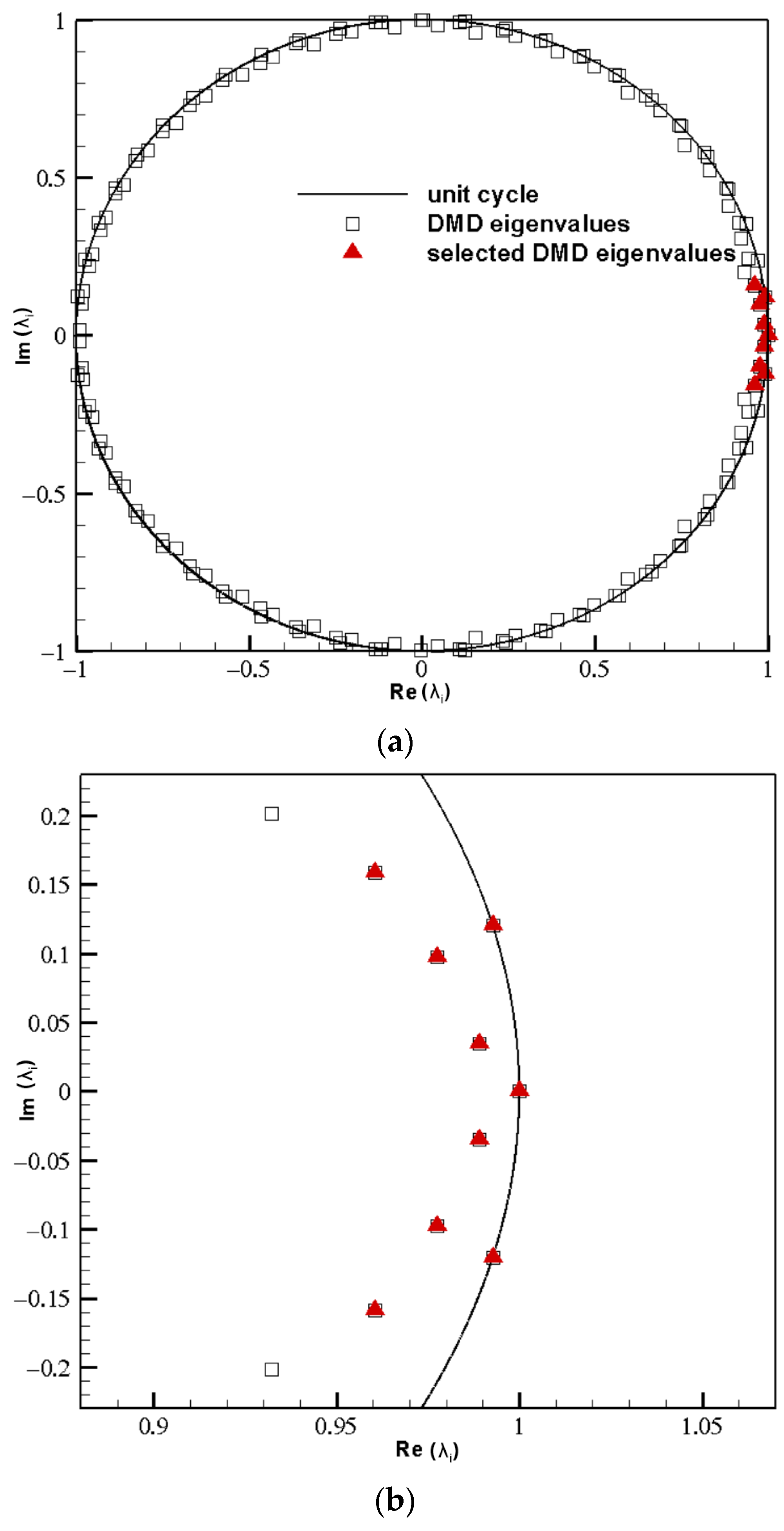
2.2. Dynamic Mode Decomposition

The Dynamic Mode Decomposition (DMD) method is used in this work, and is briefly introduced below.

DMD is a data-driven algorithm for extracting information about the flow response dynamics from experimental measurements or direct numerical simulations of flow fields [18].

A snapshot of the flow field data at the ith sampling time is obtained from experiment or numerical simulation, denoted by the vector $v_i$ ($i=1\cdots N$), $v_i\in {\Re }^{m\times 1}$, where m represents the number of physical quantities of the flow field, and N is the number of snapshots. The data shall be represented in the form of a snapshot sequence, denoted by,

$$V_1^N=\left[v_1{v}_2\cdots v_N\right]$$

(2)

We assume a linear dynamical system $A\in {\Re }^{m\times m}$, which can map the current flow field to the subsequent flow field

$$v_{i+1}=A{v}_i$$

(3)

Further, Equation (3) can also be written in terms of the entire snapshot history as

$$V_2^N=\left[v_2{v}_3\cdots v_N\right]=A\left[v_1{v}_2\cdots v_{N-1}\right]=A{V}_1^{N-1}$$

(4)

For the matrix $V_1^{N-1}$ of rank r, the goal of DMD algorithm is to find a matrix $\tilde{A}\in {ℂ}^{r\times r}$ to replace the full-order matrix $A$. This is performed via the Singular Value Decomposition (SVD) of the snapshot matrix $V_1^{N-1}$. By retaining the first r principle singular values, we have

$$A=U_r\tilde{A}{U_r}^{\ast }$$

(5)

where $U_r$ comes from the SVD of $V_1^{N-1}=U_r\Sigma {W_r}^{\ast }$. So, we have ${U_r}^{\ast }{U}_r=I$, $U_r\in {\Re }^{m\times r}$${W_r}^{\ast }{W}_r=I$, $W_r\in {\Re }^{r\times N-1}$.

Substituting Equation (5) into (4), we can obtain Equation (6),

$$A\approx \tilde{A}={U_r}^{\ast }{V}_2^N{W}_r{{\Sigma }_r}^{-1}$$

(6)

The eigendecomposition of $\tilde{A}$ then yields Ritz eigenvalues ${\lambda }_i$ and eigenvectors $y_i$ that satisfy $\tilde{A}{y}_i={\lambda }_i{y}_i$. The ith DMD mode ${\phi }_i$ is defined as

$${\phi }_i=U_r{y}_i$$

(7)

The ith DMD mode eigenvalue is defined as $g_i={\displaystyle \frac{\log \left({\lambda }_i\right)}{\Delta t}}$, and the constant sampling time $\Delta t$ is the time interval between two consecutive flow field snapshots. The real part of the eigenvalue represents the growth rate associated with this dynamic mode. A positive real part represents the growth of the mode, while a negative real part corresponds to the decay. The real part of zero indicates that the corresponding mode is stable. The imaginary part represents the modal circular frequency. In addition, it is also possible to judge that the modes are stable or not according to the r positions of the Ritz eigenvalues on the unit circle.

In terms of the eigenvalues and modes, the snapshot of the flow field at a time instance i can be expressed as below,

$$v_i={\displaystyle \sum _{j=1}^{N-1}{a}_j{\left({\lambda }_j\right)}^{i-1}{\phi }_j}=\Phi D_a{\Lambda }^{i-1}$$

(8)

where $\Phi =\left[\begin{array}{ccc}{\phi }_1& \cdots & {\phi }_{N-1}\end{array}\right]$, $D_a=\left[\begin{array}{ccc}{a}_1& & \\ & \ddots & \\ & & a_{N-1}\end{array}\right]$, $\begin{array}{l}\\ {\Lambda }^{i-1}=\left[\begin{array}{cccc}1& {\lambda }_1& \cdots & {\left({\lambda }_1\right)}^{i-1}\\ ⋮& ⋮& ⋮& ⋮\\ 1& {\lambda }_{N-1}& \cdots & {\left({\lambda }_{N-1}\right)}^{i-1}\end{array}\right]\end{array}$$a=\left[a_1{a}_2\cdots a_{N-1}\right]=Y^{+}{U_r}^{\ast }{v}_1$. Here, $a_i\left(i=1,2,\cdots N-1\right)$ denotes the amplitude of the ith mode and $Y^{+}$ denotes the Moore–Penrose pseudo inverse matrix of the matrix $Y=\left[y_1{y}_2\cdots y_{N-1}\right]$, which is the eigenvector of $\tilde{A}$.

3. Numerical Example

In this paper, an OAT15A supercritical two-dimensional airfoil with a blunt trailing edge chord length of 0.23 m was chosen as the test case. The numerical simulations were carried out with Mach 0.73, stagnation pressure 101,325 Pa, temperature 300 K, 3.5° angle of attack, and a chord-based Reynolds number of 3.2 × 10⁶. OAT15A airfoils in two cases, i.e., stationary state and pitching oscillation, were simulated and compared to analyze the main feature of the transonic buffets.

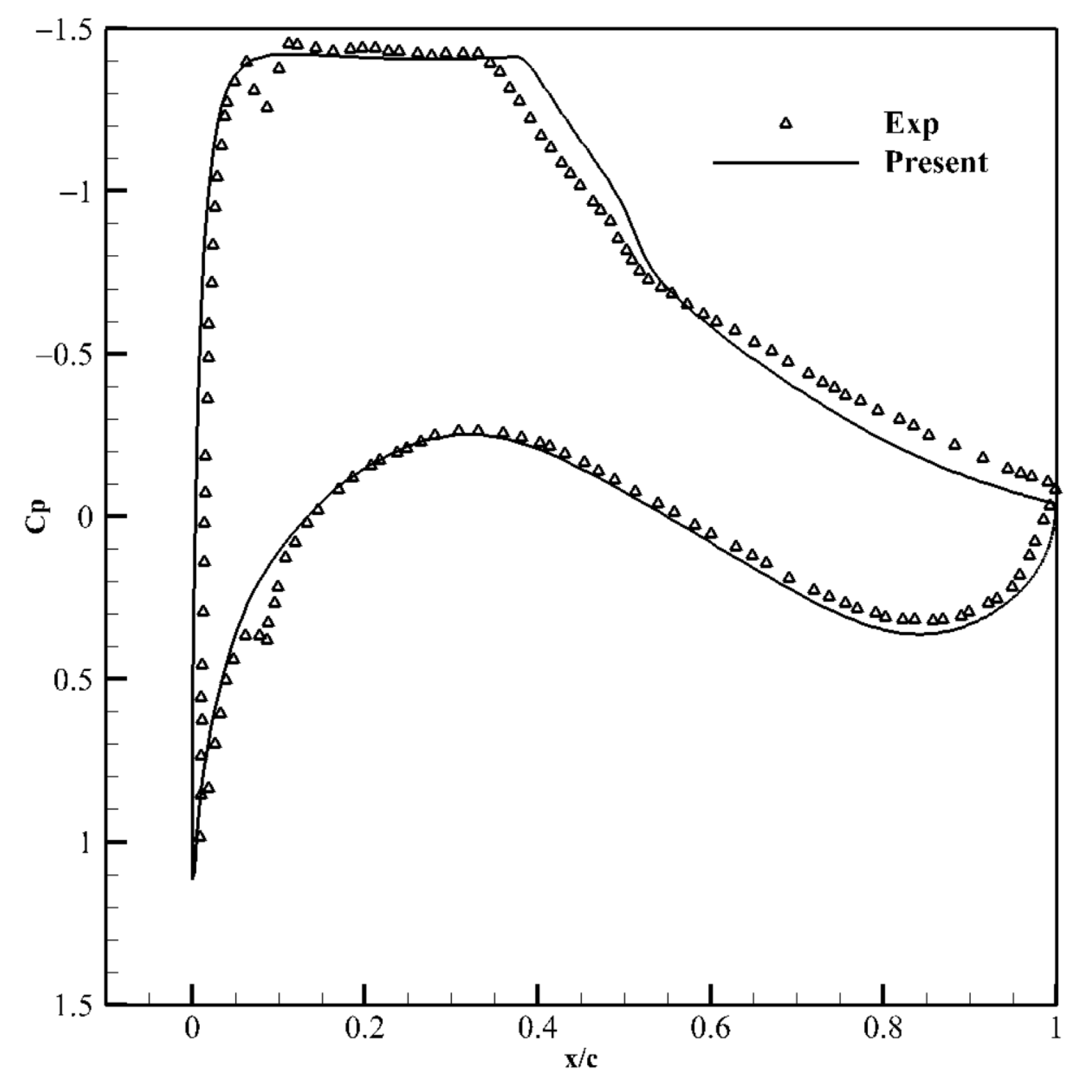
3.1. Validation of the CFD Method

Validation of the CFD computational capability of transonic buffet was performed based on a transonic buffet wind-tunnel test by Jacquin et al. [7]. The OAT15A airfoil computational grid is shown in Figure 1. The front and rear computational domains of the mesh were 30 times the chord length. A C-type structured grid was used, and 40 layers of viscous grid around the airfoil were generated. The distance between the first layer and the wall in the perpendicular direction was 5.0 × 10⁻⁶c (c is the chord length of the airfoil of 0.233 m, y⁺ is less than 1), with a mesh growth rate of 1.1, and the rest of the mesh was filled with the structured grid. The far field of the computational domain was set to the pressure far-field boundary condition, and the adiabatic no-slip boundary condition was used for the wall.

Time-averaged wall pressure coefficients were calculated using URANS with a physical time step of 6 × 10⁻⁵ s. The comparison between the computational result and the wind-tunnel experiment reported in Ref. [7] is shown in Figure 2. The present solution correlates well with the experimental data in the whole lower surface as well as in the upper surface supersonic region, and there is a slight deviation from the experiments in the pressure recovery region behind the shock wave. These results indicate that the calculation method adopted in the paper can reasonably predict the motion of the shock wave and can be applied to the subsequent simulation analysis of transonic buffet.

3.2. Flow Field Buffet Characteristics of the Fixed Airfoil

For the stationary airfoil in the transonic flow field, when the buffet occurs, the unsteady lift coefficient is shown in Figure 3a. The periodic simple harmonic motion of the shock wave causes a periodic simple harmonic change in the lift force. The Fourier transform of the lift force is shown in Figure 3b. It can be seen that the aerodynamic response is periodic and dominated by a frequency of 73 Hz. Although a double frequency is observed, its amplitude is so small that it can be ignored. Therefore, compared with the frequency 69 Hz of the lift coefficient obtained from the experiment, the error between the two is about 5.8%, which reveals that the computational method of the paper can simulate the flow field buffet accurately.

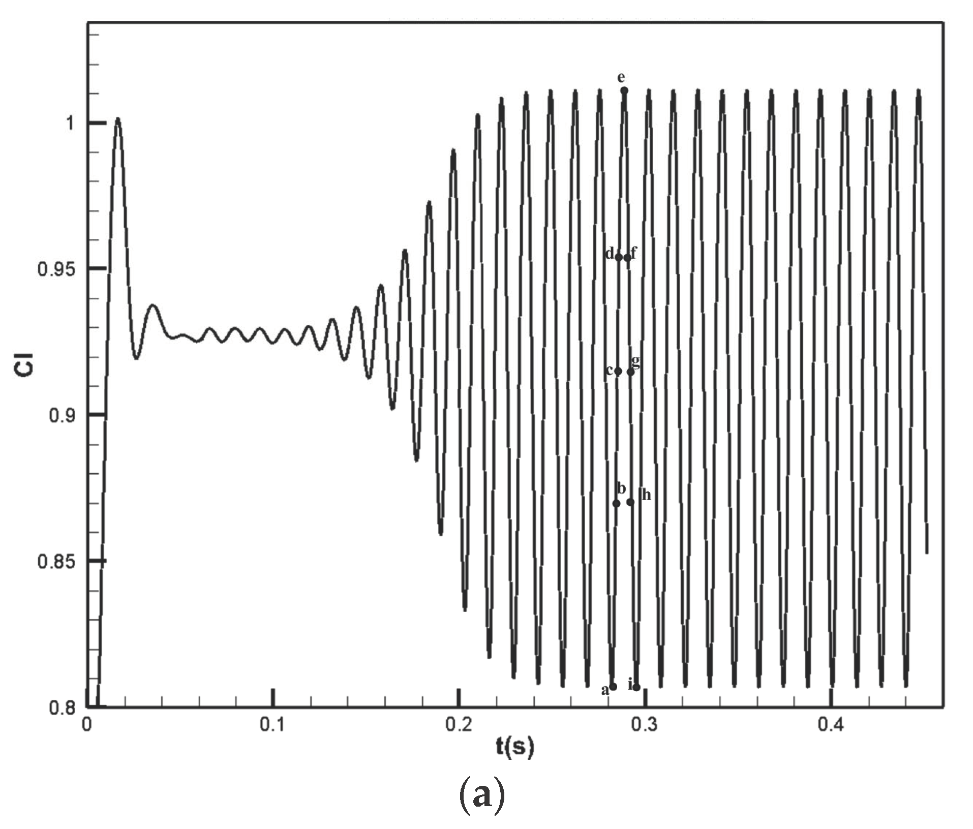
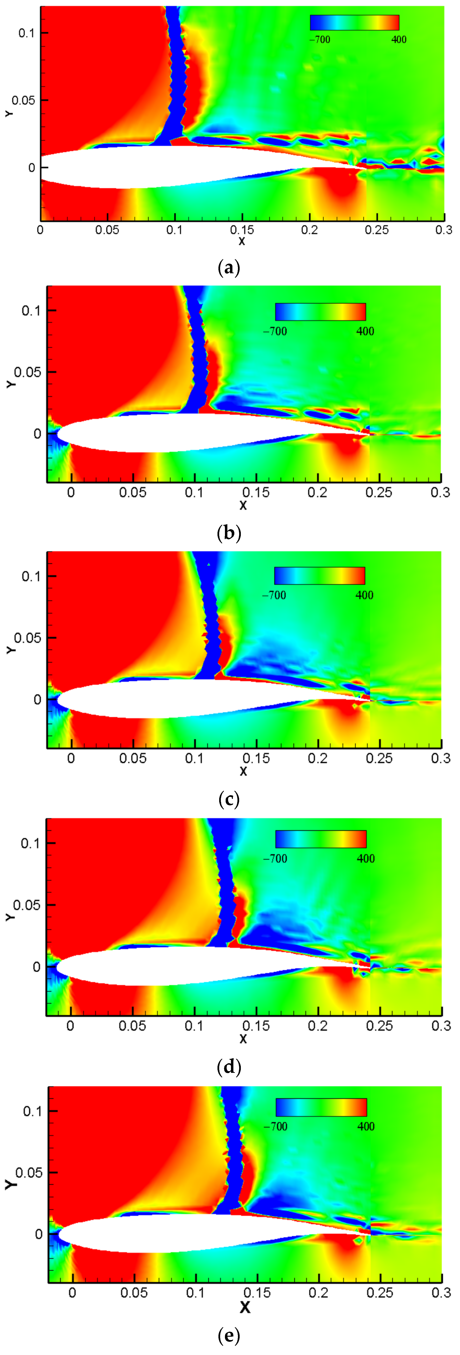
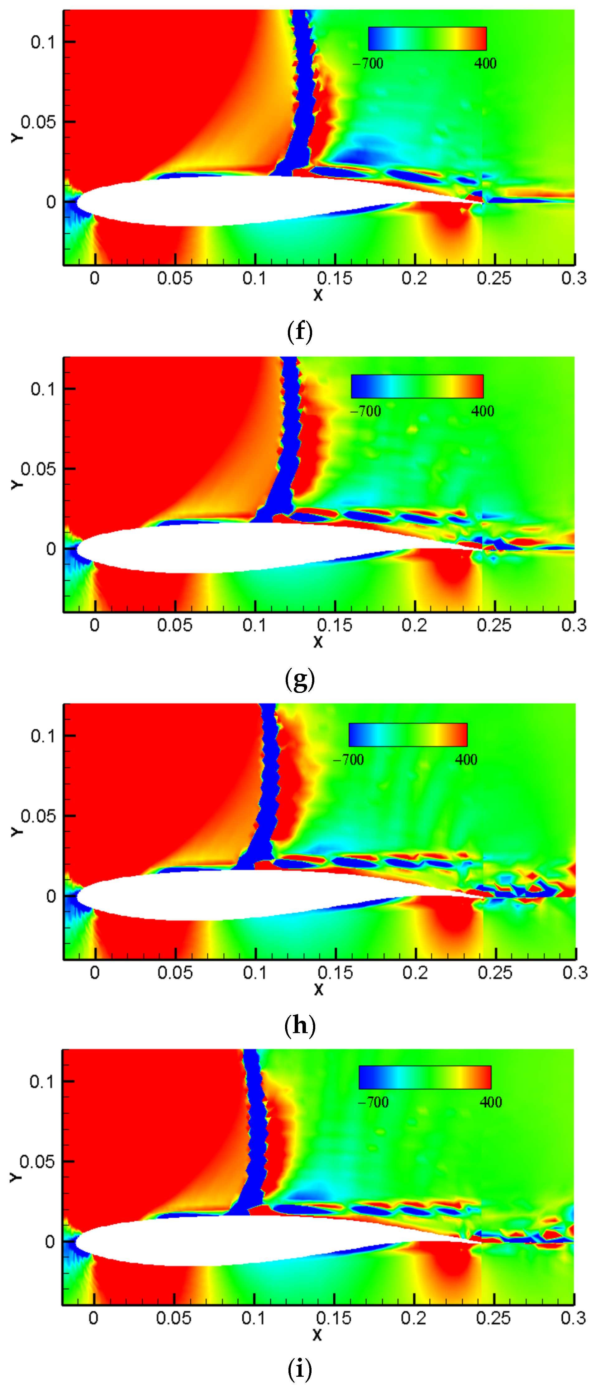
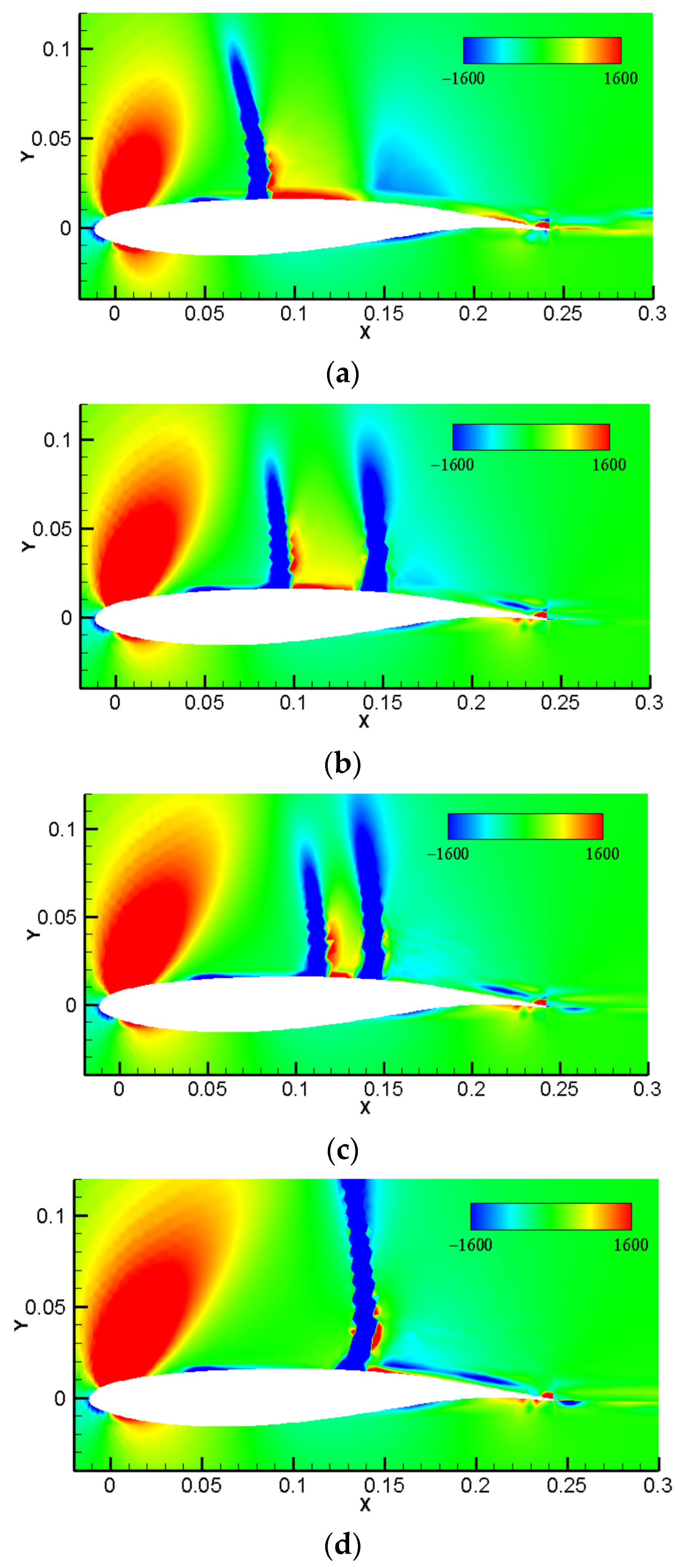
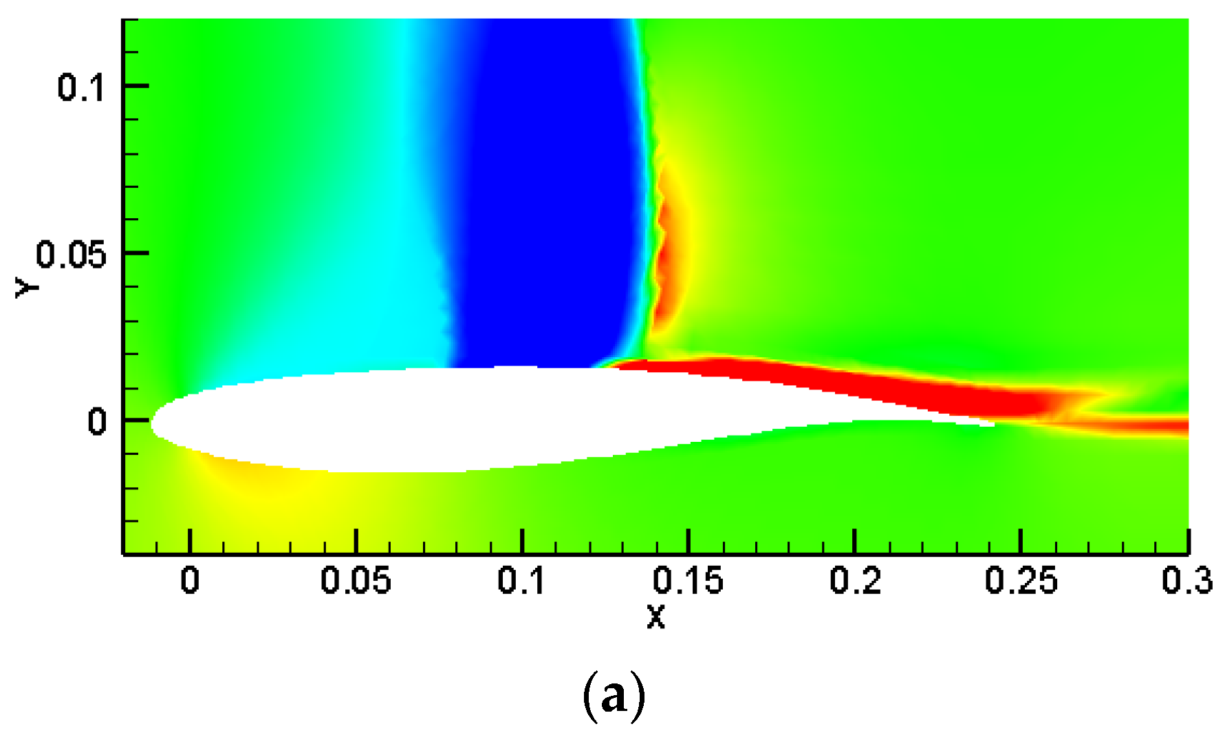
3.2.1. Instantaneous Flow Structure

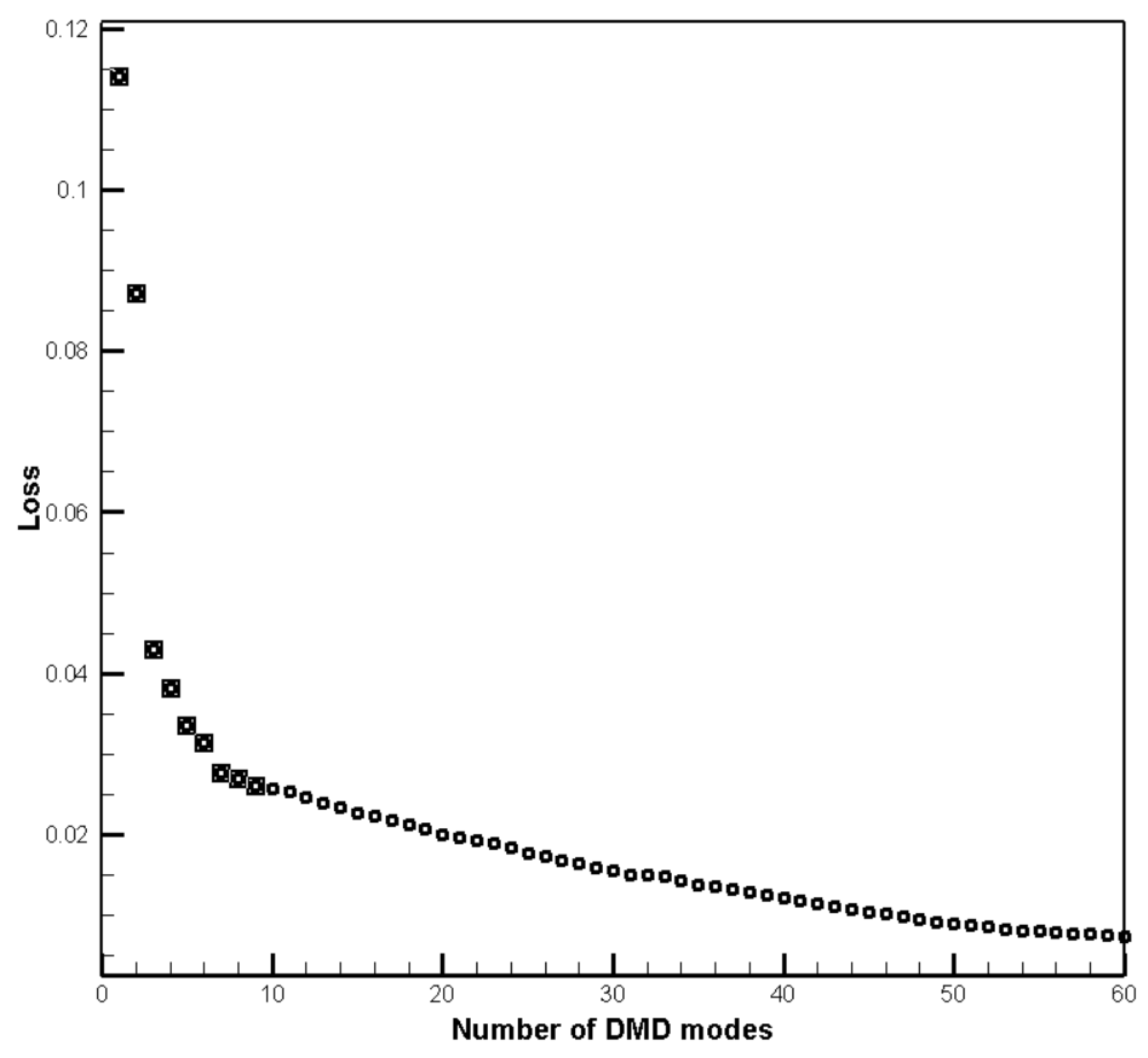
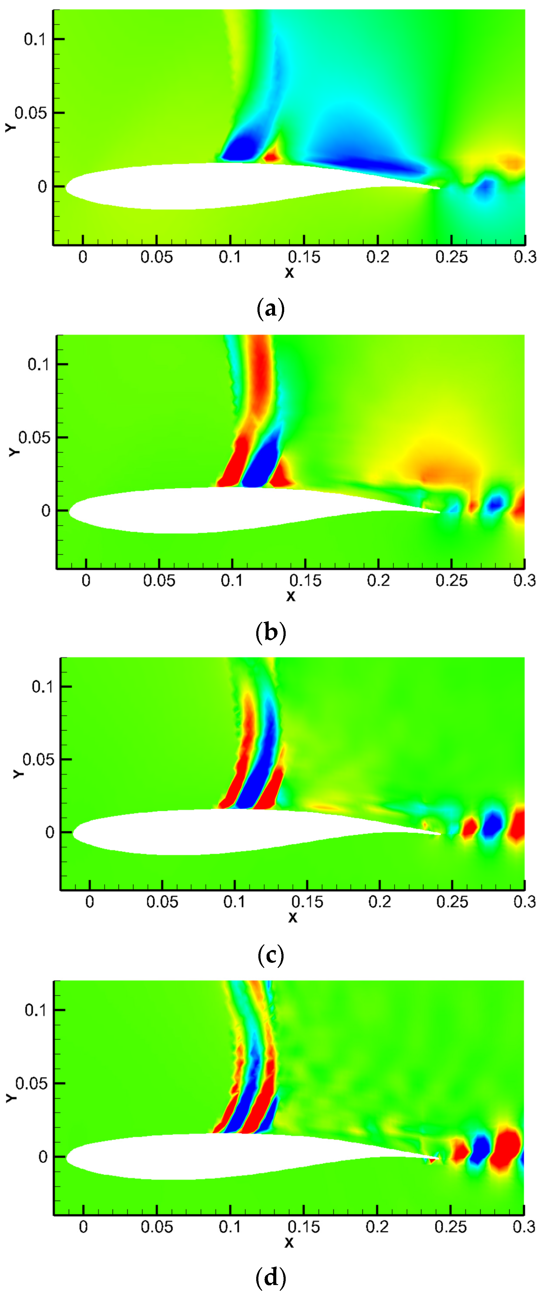
In order to study the buffet flow behavior in one period, we extracted instantaneous velocity field snapshots at nine different time points, a–i, based on URANS numerical simulation results within a buffet period, as shown in Figure 3, to investigate the flow structure of the stationary airfoil in the buffet flow.

Based on the recorded instantaneous velocity snapshots, the velocity divergency snapshots of the stationary airfoil in the transonic buffet flow field can be obtained by using the velocity divergency formula $divU={\displaystyle \frac{\partial u}{\partial x}}+{\displaystyle \frac{\partial v}{\partial y}}$, where u and v are the velocity components in the x, y directions, respectively, as shown in Figure 4. (In the following sections, unless stated, the horizontal coordinates of the flow field denote the x-axis direction coordinate parallel to the flow field, and the vertical coordinate is the y-axis direction coordinate perpendicular to the flow field, all expressed in meters.) The time at which the shock wave is located in the most upstream position is set as t₀. In Figure 4a, it can be seen that the flow separation occurs at the root of the shock, and vortex shedding structure appears. When the shock moves downstream, as shown in Figure 4b, its separated region decreases until the shock moves to its most downstream position, as illustrated in Figure 4e. Thereafter, the shock wave starts to move to the front position, and the separated region gradually increases until the shock reaches its most upstream position, as shown in Figure 4i, preparing for the next buffet period. Figure 4 shows that the transonic buffet is a self-sustained oscillation of the shock wave, and the duration time for the shock wave to move upstream is almost the same as that of its rearward movement, which is half of the buffet period.

3.2.2. Fluidic Mode

A total of 150 velocity snapshots of the flow field were collected under the computational conditions. About 50 snapshots per shock oscillation period were sampled for a total of three buffet periods. The extracted velocity snapshot samples were decomposed according to DMD to obtain the principal modes from the simulated data. These modes were employed to analyze the flow feature.

All Ritz eigenvalues can be obtained from the DMD method, and their distribution in the unit circle is shown in Figure 5a.

The modal energy criterion proposed in the literature [19,20] (shown in Equation (9)) was used to order the modes at different frequencies, according to which the modal contributions to the overall flow field were ranked.

$$I_i={\displaystyle \sum _{j=1}^{N-1}\left|a_i{\left({\lambda }_i\right)}^{j-1}\right|{‖{\phi }_i‖}_{\mathrm{F}}^2\Delta t}$$

(9)

where I_i stands for the ith order modal energy, and ${‖\bullet ‖}_{\mathrm{F}}$ is Frobenius norm. The detailed derivation and meaning of this formula can be found in [19].

The loss function defined in the literature [21], representing the error between the reconstructed flow field and the real flow field by taking the first j modes, is expressed as follows,

$${loss}_j={\displaystyle \frac{{‖V_1^N-\Phi \left(1:j\right)D_{aj}{{\Lambda }^{i-1}}_j‖}_F}{{‖V_1^N‖}_{\mathrm{F}}}}$$

(10)

where $\Phi \left(1:j\right)$ represents the first j-order modes, $D_{aj}$ represents the first j-order matrices, and ${{\Lambda }^{i-1}}_j$ represents the first j rows of ${\Lambda }^{i-1}$.

Figure 6 shows the relationship between the modes obtained by ordering the energy criterion according to Equation (9) and the loss function defined by Equation (10). In Figure 6, we can see that the first nine modes are able to maintain the loss function below 2.5%.

The distribution of the selected first nine-order modes in the unit circle is shown as the red squares in Figure 5a, and its local enlargement is shown in Figure 5b. As can be seen, all modes are basically in the vicinity of the unit circle, indicating that the system is mainly in a critical stable state under simple harmonic motion. It is also consistent with the actual physical phenomena. The growth rates and reduced frequencies of the first nine-order modes are shown in

Table 1. Dynamical parameters of extracted DMD modals of the fixed airfoil.

Order	Growth Rate	Frequency (Hz)	Loss Function
1	0	0	0.114
2–3	5.37 × 10−6	73.18	0.043
4–5	−2.45 × 10−5	146.36	0.033
6–7	6.47 × 10−5	219.56	0.027
8–9	8.38 × 10−5	293.54	0.024

, which indicates that the growth rates of the modes are very small due to the critical stable state, and the frequency of each order mode follows the buffet frequency or its higher harmonics.

The literature [18] points out that there is some phase difference between the imaginary part and the real part of the DMD mode, but the difference in the flow field characteristics is little. Based on this fact, only the real parts were analyzed for the first nine modes, as shown in Figure 5 in this paper. The modal growth rate and frequency of the first-order mode were both zero, representing the time-averaged flow field characteristics. The contours of the real parts from the remaining four pairs of conjugate modes are shown in Figure 7.

In Figure 7a, the contour displays the range of the shock motion and shock-induced separation, which is from the root of the shock to the trailing edge of the airfoil. It reveals that there are fluid modes containing shock motion and separation in the buffet flow. The contours of the real parts of the modes 4–5, 6–7, and 8–9 order show that the obvious vortex shedding structures appear in the wake, indicating that the vortex motion mode exists in the buffet flow. Modes 2–8 fully reveal that the buffet flow is the result of the interaction between the shock motion and vortex structure.

3.3. Flow Field Buffet Characteristics of Pitching Airfoils

The same flow conditions as those for the fixed airfoil were used to study the flow characteristics of the pitching airfoil when the buffet occurred. The sinusoidal pitching motion of the airfoil is given as

$$\alpha ={\alpha }_0+{\alpha }_m\sin \left(\omega t\right)$$

(11)

where ${\alpha }_0={3.5}^{\circ }$ is the mean angle of attack, ${\alpha }_m={2.2}^{\circ }$ is the maximum pitching amplitude, and ω is angular frequency set to 515 rad/s, i.e., 82 Hz, close to the buffet frequency of 73 Hz.

The temporal curves of the aerodynamic lift response to the prescribed pitch excitation are shown in Figure 8a, and its corresponding frequency content is shown in Figure 8b. From the figure, we can see that the lift response is dominated by the excitation frequency. The lift coefficient contains a main peak at the excitation frequency, with a secondary and a triple frequency that have very small amplitudes. Compared to the lift response to the fixed airfoil, the component of the buffet frequency is eliminated. It can be concluded that the aerodynamic response frequency is locked in the excitation frequency. The conclusion is consistent with Ref. [22], whereby the buffet flow response vanishes while the airfoil is oscillating at a frequency close to the buffet frequency.

3.3.1. Instantaneous Flow Structure

Compared with the stationary case of the airfoil, the shock movement phenomena in the pitching case are more complicated. In order to investigate the unsteady characteristics of the flow field during a buffet cycle, the six time instants corresponding to a–f in Figure 8a were selected, at which changes of the flow field are dramatic. The flow feature of the pitching airfoil in one period is demonstrated in Figure 9 by means of the velocity divergence snapshots corresponding to six moments.

A comparison of Figure 4 with Figure 9 demonstrates that in the pitching case, the range of the buffet separation region is larger than that in the fixed airfoil, and the regular vortex shedding of the wake in the fixed airfoil is replaced by irregular flow. Specifically, examining the flows in Figure 4a and Figure 9a together, we can see that the most upstream position of the shock wave in the flow field under pitching oscillation is more forward, starting from the chordwise position about 0.07, while that of the fixed wing case starts from the chordwise position near 0.1. Furthermore, the most downstream position of the shock wave is at the chordwise position near 0.13. It is closer to the trailing edge compared to the fixed case where it is at the chordwise position near 0.11, as displayed in Figure 4e. This observation indicates that when the structure undergoes elastic oscillation in the buffeting flow, the range of the shock wave motion is larger compared to that of the fixed structure. When the shock reaches the most upstream position and starts to move downstream, as shown in Figure 9b, a secondary shock wave is generated near the trailing edge, which is related to the interaction between the supersonic flow and the separation vortex. The secondary one continues moving upstream as the primary shock moves downstream, as seen in Figure 9c. Eventually, the two shocks meet and merge into a single one to move downstream, as depicted in Figure 9d.

In one buffet cycle, the duration time of the backward movement of the shock wave accounts for about five eighths of the buffet period, rather than half the period. It is quite different from the fixed case, where the period of the forward motion is almost the same as that of the rearward motion.

3.3.2. Fluidic Modes

The velocity snapshot samples extracted from the flow field of the pitching airfoil were decomposed by the DMD method, and the distribution of the Ritz eigenvalues in the unit circle is shown in Figure 10.

Similar to the study of the case where the airfoil is stationary in the flow field, the analysis of the flow field with the airfoil in pitching motion started with the sorting of the DMD modal orders by calculating the modal energies, and then the loss function was calculated based on the sorted modes. The relationship between the loss function and the selected modal orders is illustrated in Figure 11.

In Figure 11, it can be seen that in the pitching case, six modes were able to make the loss function less than 2%. The first nine modes were selected for the flow field analysis in the fixed airfoil case, and as a comparison, the same number of modes were also selected for airfoil pitching oscillation. The selected modal parameters are presented in

Table 2. Dynamical parameters of extracted DMD modes of the pitching airfoil.

Order	Growth Rate	Frequency (Hz)	Loss Function
1	0	0	0.061
2–3	−1.97 × 10−6	81.99	0.027
4–5	−1.08 × 10−5	163.99	0.023
6–7	−1.00 × 10−5	245.32	0.015
8–9	2.22 × 10−5	327.28	0.012

.

In Table 2, it can be seen that the first nine extracted DMD modes’ frequencies exhibit multiples of the pitching motion frequency, which implies that the structural elastic oscillation changed the characteristics of the flow field induced by buffet (shock oscillations), and the buffet flow response vanished for airfoils oscillating at a frequency close to the buffet frequency.

It can also be observed in Table 2 that among the nine modes selected, the growth rate and frequency of the first order mode are zero, representing the average flow in the flow field. We performed a flow velocity field contour analysis for the remaining four pairs of conjugate modes, and the corresponding contours of real parts are shown in Figure 12.

The shock motion and flow separation in the pitching case are given in Figure 12a,b. Figure 12b–d show that the range of shock motion is larger than that of the fixed case. In addition, the shape of the separated flow is irregular compared to the fixed case depicted in Figure 7b–d. Furthermore, there are other round-trip motions of the shock between the first and second shocks, as seen in Figure 12c,d. These observations demonstrate the complexity of the flow in this case, suggesting that structural elastic motions may play an important role in changing the feature of the buffet flow.

4. Conclusions

Numerical simulations were conducted to compute a transonic unsteady flow field around an OAT15A airfoil that was in stationary and harmonically pitching conditions in a transonic buffeting flow, using the URANS method with the sst-kω model. Velocity divergence snapshots and the DMD method were employed to investigate the unsteady aerodynamics and the feature of the flows. The main conclusions are as follows:

(1)

When the airfoil is in pitching motion, the oscillation frequency has a significant effect on the flow characteristics. If the pitching frequency is close to the buffeting frequency of the flow, the aerodynamics may manifest as a harmonic vibration with only the pitching frequency of the structure as the fundamental frequency, and the frequency of the flow field disappears.

(2)

Velocity divergence snapshots show that for a given pitching motion, compared with the corresponding buffet characteristics of the stationary airfoil, the interaction of two shocks exists in the former, which leads to an increased range of shock motion. The wake shows obvious disordered motions compared with that of the latter, which results in a more complex unsteady shock behavior of the flow under elastic oscillation.

(3)

The DMD modes extracted by ordering the modes at different frequencies according to the modal energy criterion can obtain the principal modes, which reflectthe periodicity of the transonic shock oscillations, and facilitate the study of the dominant mode characteristics in the periodic flow.

References

1. Dolling, D. Fifty years of shock-wave/boundary-layer interaction research: What next? AIAA J. 2001, 39, 517–1531. [Google Scholar] [CrossRef]
2. Lee, B.H.K. Oscillatory shock motion caused by transonic shock boundary-layer interaction. AIAA J. 1990, 28, 942–944. [Google Scholar] [CrossRef]
3. Lee, B.H.K. Self-sustained shock oscillations on airfoils at transonic speeds. Prog. Aerosp. Sci. 2001, 37, 147–196. [Google Scholar] [CrossRef]
4. Xiao, Q.; Tsai, H.M.; Liu, F. Numerical study of transonic buffet on a supercritical airfoil. AIAA J. 2006, 44, 620–628. [Google Scholar] [CrossRef]
5. Crouch, J.D.; Garbaruk, A.; Magidoy, D. Predicting the onset of flow unsteadiness based on global instability. J. Comput. Phys. 2007, 224, 924–940. [Google Scholar] [CrossRef]
6. Crouch, J.D.; Garbaruk, A.; Magidoy, D.; Travin, A. Origin of transonic buffet on airfoils. J. Fluid Mech. 2009, 628, 357–369. [Google Scholar] [CrossRef]
7. Jacquin, L.; Molton, P.; Deck, S.; Maury, B.; Soulevant, D. Experimental study of shock oscillation over a transonic supercritical profile. AIAA J. 2009, 47, 1985–1994. [Google Scholar] [CrossRef]
8. Masini, L.; Timme, S.; Ciarella, A.; Peace, A. Influence of vane vortex generators on transonic wing buffet: Further analysis of the BUCOLIC experimental dataset. In Proceedings of the 52nd 3AF International Conference on Applied Aerodynamics, Lyon, France, 17–19 March 2017. [Google Scholar]
9. Nitzsche, J. A numerical study on aerodynamic resonance in transonic separated flow. In Proceedings of the International Forum on Aeroelasticity and Structural Dynamics, Seattle, WA, USA, 22–24 June 2009. [Google Scholar]
10. Gao, C.Q.; Zhang, W.W.; Ye, Z.Y. Study on the effects of elastic characteristics on transonic buffet onset. Eng. Mech. 2017, 34, 243–247. [Google Scholar]
11. Zhang, W.W.; Gao, C.Q.; Ye, Z.Y. Research advances of wing/airfoil transonic buffet. Acta Aeronaut. Astronaut. Sin. 2015, 36, 1056–1075. [Google Scholar]
12. Raveh, D.E. Numerical study of an oscillating airfoil in transonic buffeting flows. AIAA J. 2009, 47, 505–515. [Google Scholar] [CrossRef]
13. Raveh, D.E.; Dowell, E.H. Frequency lock-in phenomenon for oscillating airfoils in buffeting flows. J. Fluids Struct. 2011, 27, 89–104. [Google Scholar] [CrossRef]
14. Raveh, D.E.; Dowell, E.H. Aeroelastic responses of elastically suspended airfoil systems in transonic buffeting flows. AIAA J. 2014, 52, 926–934. [Google Scholar] [CrossRef]
15. Gao, C.Q.; Zhang, W.W. Transonic aeroelasticity: A new perspective from the fluid mode. Prog. Aerosp. Sci. 2020, 113, 1–19. [Google Scholar] [CrossRef]
16. Han, B.; Xu, M.; Chen, G.G.; Cai, T.X.; Wang, W.H.; Guan, S.X. Numerical investigation of transonic buffet on a prescribed-pitching OAT15A airfoil. AIP Adv. 2022, 12, 035301. [Google Scholar] [CrossRef]
17. Nie, X.Y. Numerical analysis of geometrical nonlinear aeroelasticity with CFD/CSD method. Int. J. Nonlinear Sci. Numer. Simul. 2021, 22, 243–253. [Google Scholar] [CrossRef]
18. Kou, J.Q.; Zhang, W.W.; Gao, C.Q. Modal analysis of transonic buffet based on POD and DMD method. Acta Aeronaut. Astronaut. Sin. 2016, 37, 2679–2689. [Google Scholar]
19. Kou, J.Q.; Zhang, W.W. An improved criterion to select dominant modes from dynamic mode decomposition. Eur. J. Mech. B Fluids 2017, 62, 109–129. [Google Scholar] [CrossRef]
20. Jovanovic, M.R.; Schmidp, J.; Nicholsj, W. Sparsity-promoting dynamic mode decomposition. Phys. Fluids 2014, 26, 024103. [Google Scholar] [CrossRef]
21. Kou, J.Q.; Zhang, W.W. Dynamic mode decomposition with exogenous input for data-driven modeling of unsteady flows. Phys. Fluids 2019, 31, 057106. [Google Scholar] [CrossRef]
22. Gao, C.Q.; Zhang, W.W.; Li, X.T.; Liu, Y.; Quan, J.; Ye, Z.; Jiang, Y. Mechanism of frequency lock-in transonic buffeting flow. J. Fluid Mech. 2017, 88, 528–561. [Google Scholar] [CrossRef]
Figure 1. Computational grid. (a) Overview of computational grid. (b) Close-up view of the airfoil.
Applsci 14 07149 g001
Figure 2. Comparison results of airfoil time-averaged pressure coefficient between the simulation and experiment.
Applsci 14 07149 g002
Figure 3. Flow lift coefficient of the fixed airfoil. (a) Lift coefficient time history (a–i stand for different time points). (b) Frequency content of the lift coefficient.
Applsci 14 07149 g003aApplsci 14 07149 g003b
Figure 4. Snapshots of instantaneous velocity divergence in one buffet period for the fixed airfoil. (a) t = t0. (b) t = t0 + T/8. (c) t = t0 + T/4. (d) t = t0 + 3/8T. (e) t = t0 + T/2. (f) t = t0 + 5/8T. (g) t = t0 + 3/4T. (h) t = t0 + 7/8T. (i) t = t0 + T.
Applsci 14 07149 g004aApplsci 14 07149 g004b
Figure 5. DMD modal eigenvalues of the fixed airfoil. (a) The distribution of all eigenvalues in unit circle. (b) The distribution of first 9 modal eigenvalues extracted in unit circle.
Applsci 14 07149 g005
Figure 6. Relationship of the loss function with the numbers of selected DMD orders for fixed airfoil.
Applsci 14 07149 g006
Figure 7. The first 4 pairs of conjugate modal contours of streamwise velocity for the fixed airfoil. (a) DMD modes 2–3. (b) DMD modes 4–5. (c) DMD modes 6–7. (d) DMD modes 8–9.
Applsci 14 07149 g007
Figure 8. Flow lift coefficient of pitching airfoil. (a) Lift coefficient time history (a–f stand for different time points). (b) Frequency content of the lift coefficient.
Applsci 14 07149 g008
Figure 9. Snapshots of instantaneous velocity divergence in one buffet period for the pitching airfoil. (a) t = t0. (b) t = t0 + T/8. (c) t = t0 + 4/8T. (d) t = t0 + 5/8T. (e) t = t0 + 6/8T. (f) t = t0 + T.
Applsci 14 07149 g009aApplsci 14 07149 g009b
Figure 10. DMD modal eigenvalues of pitching airfoil. (a) The distribution of all eigenvalues in the unit circle. (b) The distribution of first 9 modal eigenvalues extracted in unit circle.
Applsci 14 07149 g010
Figure 11. Relationship of the loss function with the numbers of DMD orders in pitching airfoil.
Applsci 14 07149 g011
Figure 12. The first 4 pairs of conjugate modal real part contours of streamwise velocity for the pitching airfoil. (a) DMD modes 2–3. (b) DMD modes 4–5. (c) DMD modes 6–7. (d) DMD modes 8–9.
Applsci 14 07149 g012aApplsci 14 07149 g012b