Optimizing Supply Chain Efficiency Using Innovative Goal Programming and Advanced Metaheuristic Techniques

Abstract

This paper presents an optimization approach for supply chain management that incorporates goal programming (GP), dependent chance constraints (DCC), and the hunger games search algorithm (HGSA). The model acknowledges uncertainty by embedding uncertain parameters that promote resilience and efficiency. It focuses on minimizing costs while maximizing on-time deliveries and optimizing key decision variables such as production setups, quantities, inventory levels, and backorders. Extensive simulations and numerical results confirm the model’s effectiveness in providing robust solutions to dynamically changing supply chain problems when compared to conventional models. However, the integrated model introduces substantial computational complexity, which may pose challenges in large-scale real-world applications. Additionally, the model’s reliance on precise probabilistic and fuzzy parameters may limit its applicability in environments with insufficient or imprecise data. Despite these limitations, the proposed approach has the potential to significantly enhance supply chain resilience and efficiency, offering valuable insights for both academia and industry.

1. Introduction

In current logistics, supply chain management (SCM) is very important because it ensures that products are moved efficiently and smoothly from their manufacturers to consumers across international boundaries [1,2]. It is therefore essential that these worldwide supply chains are optimized to guarantee both recovery and efficiency in terms of cost and time. In the current condition of Industry 4.0, the dynamic and uncertain supply chain makes the old school of deterministic models limited in handling volatile conditions [3]. These models seldom account for uncertainties like demand changes, disruptions, or variations in lead times, yet all these are critical to the overall performance of the supply chain [4,5].

To overcome the constraints above, recent developments have centered on amalgamating probabilistic and fuzzy decision-making methodologies. Probabilistic models enable deeper insight into uncertainties and variabilities by embracing the chances of different events taking place, while fuzzy logic plays a role in managing imperfect and uncertain input, reflecting real-life situations more appropriately [6]. These approaches represent a significant departure from deterministic models and offer greater robustness and flexibility for supply chain operations.

To further enhance decision-making in supply chain management (SCM), it is advisable that uncertainty theory be employed. This principle states that the risks within supply chains should be incorporated into stochastic, fuzzy logic processes to build stronger and more flexible systems [7].

Superior overall performance of the supply chain necessitates this improvement in risk management as well as informed decision-making [8]. As supply chains continue to grow and change, it becomes increasingly important to use optimization models that are capable of managing these complexities [9].

In this changing environment, goal programming (GP) stands out as a powerful multi-objective optimization technique. Charnes and Cooper [10] first introduced it more than fifty years ago. Its flexibility and effectiveness make it especially valuable within the complex and fluctuating landscape of supply chains. GP enables decision-makers to address multiple, often conflicting objectives simultaneously [10].

To improve optimization models, dependent chance constraints (DCC) are used to capture how different uncertain parameters depend on each other. By considering the joint distribution of uncertain factors, DCC-based models [11] offer holistic risk management, significantly enhancing optimization in supply chains [6]. This integration allows for more accurate and reliable optimization results, reflecting real-world conditions.

Metaheuristic algorithms such as the hunger games search algorithm (HGSA) [12] and genetic algorithms (GA) [13] further strengthen optimization. Inspired by natural processes, these algorithms excel in exploring and exploiting multi-dimensional solution spaces, making them ideal for modern supply chains. HGSA mimics foraging behavior among animals, while GA simulates natural selection processes. Both algorithms improve the performance of supply chain optimization by making them more adaptive and efficient ([14,15]).

In this context, the current study has developed a novel optimization model that synergizes goal programming (GP), dependent chance constraints (DCC), and the hunger games search algorithm (HGSA). This model optimizes critical decision variables such as production setups, quantities produced, inventory levels, and backorders to minimize costs and maximize on-time deliveries. The 99-method is used in several numerical analyses and simulations, showing substantial improvements in cost efficiency and delivery performance. This integrated approach, therefore, provides a solid foundation for addressing contemporary supply chain challenges.

In this paper, Section 2 provides an overview of previous research conducted in the field of optimized supply chains; Section 3 gives details about the proposed model, including its mathematical formulation and how it integrates goal programming (GP), dependent chance constraints (DCC), and the hunger games search algorithm (HGSA). In Section 4,the simulation setup will be discussed, including the parameters used in the numerical analysis. In Section 6, we will present the results comparing the performance of the proposed model with traditional deterministic models. Section 7 will summarize the major findings, discuss practical implications, and suggest areas for future work.

2. Theoretical Background of the Uncertainty Theory

Optimizing a supply chain means aligning various supply chain elements to improve performance. Some well-known optimization procedures, such as linear programming (LP) and mixed-integer linear programming (MILP), assume a particular environment. However, deterministic models are currently limited in their ability to support decision-making in uncertain situations characterized by dynamism and a lack of historical data [16].

2.1. Uncertainty Theory: Measure, Variable, and Distribution

Uncertainty theory involves modeling non-random uncertainty using concepts such as uncertain measures, variables, or distributions. It is crucial for understanding the variability that is always present and the impossibility of predicting supply chain orders.

2.1.1. Uncertainty Measures

Uncertainty measures have been applied in a variety of SCM contexts, such as the quantification of uncertainty in lead time, demand forecasting, and supplier reliability. Recent research has shown that these techniques can be used to develop more flexible supply chain strategies by incorporating uncertainty into inventory, purchasing, and logistics planning [6,16]. An uncertainty measure is a set function $\mathcal{M}$ on some sample space that assigns numbers from 0 to 1 and satisfies the axioms of normality, duality, sub-additivity, and product measure, providing a precise analysis regarding the possibility of something uncertain.

For instance, in the context of supply chains, uncertainty quantifies the likelihood of late deliveries, demand fluctuations, etc. An uncertainty measure $\mathcal{M}$ on a sigma-algebra $\mathcal{F}$ over the set T is defined mathematically by the following equation:

• Normality: $\mathcal{M}\left(T\right)=1$
• Duality: $\mathcal{M}\left(A\right)+\mathcal{M}\left(A^c\right)=1$ for any $A\subseteq T$
• Sub-additivity: $\mathcal{M}\left({\bigcup }_{i=1}^{\infty }{A}_i\right)\le {\sum }_{i=1}^{\infty }\mathcal{M}\left(A_i\right)$
• Product Measure: $\mathcal{M}(A\cap B)=\mathcal{M}\left(A\right)·\mathcal{M}\left(B\right)$ for independent events A and B

2.1.2. Uncertain Variables

Uncertain variables have been used to model demand fluctuations, supply chain disturbances, and deployment time fluctuations in SCM. Advanced applications include dynamic pricing models, where uncertain variables represent market demand, and inventory management systems that adjust stock levels based on uncertain times and demand patterns [6,17]. In the domain of uncertainty, an uncertain variable is a function that maps outcomes from uncertainty spaces onto real numbers. Any Borel set B must be measurable, meaning it must belong to the sigma-algebra of an event set $\{\xi \in B\}$. This concept is useful when discussing logistics elements that typically lack precise calculations, such as demand, supply, and order fulfillment periods.

In other words, an uncertain variable $\xi$ is a mapping or correspondence from the uncertainty space $(T,\mathcal{F},\mathcal{M})$ to the set of real numbers, such that the pre-image of each Borel set B, where $\{\xi \in B\}$, is in $\mathcal{F}$.

2.1.3. Uncertainty Distribution

The uncertainty distribution is used to model the likelihood of various outcomes in SCM, such as demand rates or delivery times. This classification supports risk assessment and decision-making processes, enabling better preparedness for different scenarios. Recent developments include the use of uncertainty classification in predictive analytics to develop demand forecasts and risk management strategies to improve supply chain resilience [18,19]. Defining the ’uncertain variable’ $\xi$, which has an uncertainty distribution $\Phi \left(x\right)$ given by $\Phi \left(x\right)=\mathcal{M}(\xi \le x)$, the distribution measures the event where $\xi$ is less than or equal to a value x. For regular uncertainty distributions, the values mainly range between 0 and 1 and are continuous and strictly increasing. Bias is absent in the linear asymmetry of $\xi$, and it can be expressed as follows:

$$\Phi \left(x\right)=\left\{\begin{array}{cc}0,\hfill & \mathrm{if}x<a\hfill \\ {\displaystyle \frac{x-a}{b-a}},\hfill & \mathrm{if}a\le x\le b\hfill \\ 1,\hfill & \mathrm{if}x>b\hfill \end{array}\right.$$

where a and b are constants with $a<b$.

2.2. Dependent Chance Programming Model

The use of a dependent chance programming (DCP) model in SCM seeks to optimize supply chain networks under correlated risks, such as multiple suppliers or transportation times. Recent studies have used DCP models to improve the robustness of production planning and distribution systems by accounting for supply chain uncertainty [6,20]. Unlike conventional models, which assume independent random variables, DCP considers interdependencies among uncertain parameters—extending traditional deterministic models into stochastic ones. By taking the joint distribution of uncertainties into consideration, DCP helps improve decision-making under correlated risks. For example, a holistic approach might be needed for both production schedules and delivery times when an interruption in raw material supply affects them simultaneously [20].

Mathematical Formulation of DCP

The DCP model optimizes decision variables x by combining both deterministic and probabilistic constraints. Typically, the objective function to be minimized is a combination of deterministic costs as well as expected costs due to uncertainties.

$$\mathrm{Minimize}Z=f\left(x\right)+\sum _{i=1}^n\mathbb{E}\left[C_i\left(\xi \right)\right]$$

The notation $f\left(x\right)$ is used when discussing deterministic parts of an expression, whereas $\mathbb{E}\left[C_i\left(\xi \right)\right]$ represents uncertain costs. Probabilistic constraints are necessary to guarantee the operation of the system in cases where it is impossible to determine something precisely. They ensure certain performance levels under uncertainty:

$$Pr\{h_k(x,\xi )\le d_k\}\ge {\alpha }_k,\forall k$$

where $h_k(x,\xi )$ represents the probabilistic constraints, $d_k$ are thresholds, and ${\alpha }_k$ are acceptable probabilities that satisfy the constraints.

The model represents relationships between the parameters using copulas or joint probability distributions. For example, their joint distribution is denoted as $Pr({\xi }_1,{\xi }_2)$ when ${\xi }_1$ and ${\xi }_2$ are dependent uncertain parameters.

2.3. Goal Programming and Simulation using Uncertainty (99-Method)

Goal programming (GP) has been applied to SCM for multi-objective optimization, balancing cost, service levels, and inventory levels [10,18]. GP is an approach to deal with multiple, frequently contradictory goals through optimization, aimed at minimizing deviations from the predetermined levels of performance [21]. Specifically, it introduces variables to measure the extent to which goals are met or not met, thereby enabling stakeholders to navigate the trade-offs between various dimensions of operation within logistics [10].

2.3.1. Mathematical Formulation of GP

In GP, each goal $g_i\left(x\right)$ with target $t_i$ is formulated as follows:

$$g_i\left(x\right)+d_i^{-}-d_i^{+}=t_i,\forall i$$

In this case, $d_i^{-}$ and $d_i^{+}$ are the variables representing deviations less than and greater than the target, respectively. The goal is to minimize the sum of these deviations, weighted by a non-negative number:

$$\mathrm{Minimize}Z=\sum _{i=1}^m(w_i^{+}{d}_i^{+}+w_i^{-}{d}_i^{-})$$

subject to the constraints $g_i\left(x\right)+d_i^{-}-d_i^{+}=t_i$ and $x\in X$, where $w_i^{+}$ and $w_i^{-}$ are the weights assigned to the deviations, and X is the feasible region.

2.3.2. Simulation under Uncertainty: 99-Method

To evaluate supply chain performance under different scenarios, the 99-method is used to test various situations. Risks are accurately identified, and measures are implemented to counteract disruptions, thereby boosting supply chain resilience.

In practice, the 99-method can model scenarios such as fluctuations in demand, supply interruptions, and shifts in transit times. Such simulations help in ascertaining the impact of these uncertainties on supply chain operations and in creating resilient policies to address them [18].

2.4. Applications and Benefits of Uncertain Models

Models that incorporate uncertain phenomena such as probability, fuzziness, and randomness are better-suited to handle variable supply and demand patterns over time, leading to improved optimization. Major methodologies like stochastic programming (SP), fuzzy logic (FL), and robust optimization (RO) are often considered to enhance the resilience and efficiency of supply chains [6].

2.4.1. Stochastic Programming (SP)

Stochastic programming (SP) has been widely used in supply chain management, particularly in inventory management, capacity planning, and transportation management. Recent research has applied SP to develop robust methods that account for demand variability, supply chain disruptions, and other uncertainties, thereby enhancing overall supply chain flexibility and efficiency [17,19]. SP problems are addressed by considering multiple scenarios and their associated probabilities. This technique is effective in contexts such as controlling stock levels when sales volumes are uncertain over a given period or determining manufacturing production levels when rates are uncertain during specific periods [17]. One way to formulate the SP model is through the following:

$$\mathrm{Minimize}\sum _{s\in S}{p}_s{C}_s\left(x_s\right)$$

subject to:

$$\sum _{j\in J}{a}_{ij}{x}_{js}\ge b_{is},\forall i,\forall s$$

Depending on the circumstances S belongs to, $p_s$ is the probability that scenario s will occur, $C_s\left(x_s\right)$ represents the cost when the occurrence is scenario-specific, $a_{ij}$ are the coefficients, and $b_{is}$ are scenario-specific constraints.

2.4.2. Fuzzy Logic (FL)

Fuzzy logic (FL) is used in SCM for supplier selection, risk analysis, and demand forecasting. FL models help address the ambiguity and imprecision inherent in these decisions, resulting in more flexible supply chain strategies. Recent developments include the integration of FL with other strategies to improve decision-making under uncertainty [6,19]. Fuzzy logic deals with uncertain or vague circumstances by creating imprecise collections of data relevant to activities such as choosing vendors, predicting consumer interest, and making decisions when no single solution is definitive [6]. For instance, it might be represented as follows:

$$A\left(x\right)={\mu }_A\left(x\right)\ge \alpha$$

where $A\left(x\right)$ is a fuzzy set, ${\mu }_A\left(x\right)$ is the membership function, and $\alpha$ is the minimum acceptable level.

2.4.3. Robust Optimization (RO)

Robust optimization (RO) has been used to develop resilient supply chains in the face of natural disasters or market fluctuations. The RO process helps devise strategies to maintain operations under various uncertain conditions, thereby increasing supply chain efficiency and reliability. Recent research has focused on improving the computational performance of RO models and integrating them with real-time data analysis [18,19]. Robust optimization is particularly useful in scenarios involving potential manufacturers facing worst-case conditions, such as network design, inventory creation, and production scheduling. This concept helps address the uncertainties and peculiarities facing the supply chain [18]. The formulation of the model under robust optimization is as follows:

$$\mathrm{Minimize}f\left(x\right)$$

subject to:

$$g_i(x,\xi )\le 0,\forall \xi \in \Xi ,\forall i$$

where $g_i(x,\xi )$ are the constraints affected by uncertainty $\xi$, and $\Xi$ is the uncertainty set.

Metaheuristic Algorithms

The use of fuzzy decision-making processes in supply chain management (SCM) has been well-documented, allowing for better management of uncertainty and improved communication complexity within supply chains. Recent developments in metaheuristic algorithms, such as the genetic algorithm (GA), particle swarm optimization (PSO), ant colony optimization (ACO), and hunger games search algorithm (HGSA), have shown great promise in enhancing SCM performance and robustness. These algorithms are designed to find near-optimal solutions to complex problems by efficiently searching large solution spaces.

GA, inspired by natural selection, has been successfully used to optimize multi-level conservation systems, resulting in significant cost reductions and service level improvements [22]. PSO, based on the social behavior of birds and fish, has been effectively applied to dynamic vehicle routing and warehouse location planning, achieving better delivery times and reduced operational costs [23]. ACO, by simulating bee feeding behavior, has been used to solve combinatorial optimization problems, improving distribution efficiency and reducing costs in distribution networks [24]. Additionally, hybrid methods that combine different algorithms, such as GA-PSO, have gained traction, resulting in improved solution quality and computational efficiency [25]. Recent advancements focus on increasing convergence speed, solution quality, and robustness through parallel and distributed computing techniques, making these algorithms suitable for large-scale SCM problems. Furthermore, the integration of machine learning techniques with metaheuristics has opened new possibilities for adaptive and intelligent optimization, greatly enhancing supply chain operations and efficiency [26,27]. The effectiveness of HGSA in optimizing supply chain performance under uncertainty has been demonstrated, highlighting the potential of advanced metaheuristic techniques in designing robust supply chain strategies [28].

3. Supply Chain Mathematical Model

Improving supply chain quality involves aligning multiple variables to track performance and efficiency [29]. This section describes the mathematical models used in supply chain management and emphasizes how they incorporate uncertainty, contingency-based models, and assumptions under uncertainty. A comprehensive analysis of the proposed model’s performance ensures the selection of appropriate case studies and scenarios for simulations. Various delivery systems, including single-layer and multi-layer communication, were evaluated to assess the model’s applicability across different systems [30]. Scenarios were chosen to reflect heterogeneous demand and supply uncertainties, encompassing a range of environments and complexities.

3.1. Uncertainty Theory: Measure, Variable, and Distribution

Uncertainty theory provides a mathematical framework for modeling non-random uncertainty through unpredictable measures, variables, and distributions. This is significant for representing the inherent randomness and volatility of supply chain parameters.

3.2. Supply Chain Network Configuration

The supply chain network considered in this study includes suppliers, manufacturers, distribution centers, and consumers, with each node playing a crucial role in the sourcing and final delivery of goods. Case studies across different geographies and industries incorporate varying complexities in decision variables such as manufacturing processes, volume, inventory levels, and layout. Factors like demand levels, production capacity, and transportation infrastructure also influence the model. Scenarios with reliable historical data were prioritized, as data quality and availability are critical for a well-documented supply chain. The selected scenarios reflect real-world challenges such as demand forecasting, supply reliability, transportation delays, and inventory balances, ensuring the findings are applicable to practical situations.

3.2.1. Uncertain Supply Chain Network Optimization Problem

Optimizing supply chain networks (SCNs) involves addressing the intricate combinatorial optimization problem of managing the movement of goods across multiple nodes under uncertainty. These nodes include suppliers, manufacturers, distribution centers, and customers. The key variables and assumptions are outlined below.

3.2.2. Key Variables and Hypothesis

Effective supply chain management requires a thorough understanding of the dynamic factors affecting its efficiency and robustness. To enhance supply chain performance under uncertainty, it is crucial to identify and measure the key variables that influence decision-making. The following key variables have been identified as critical to our integrated model.

• Key Variables

To effectively model and optimize supply chain operations under uncertainty, it is essential to identify the fundamental variables that impact performance. These key variables form the foundation of our integrated model, capturing the core elements of supply chain dynamics.

• Demand rates: These determine the quantity of products required by end consumers and are assumed to be uncertain random variables.
• Supply availability: This indicates the availability of raw materials and finished goods, which are also subject to uncertainty.
• Production capacity: This defines the maximum output of manufacturing facilities and can vary based on several factors.
• Transportation logistics: This encompasses the movement of goods between different nodes in the supply chain and is influenced by various uncertainties.

• Hypotheses

To ensure the robustness of our model, we test the following additional hypotheses related to the operational aspects of the supply chain:

• All supply chain nodes are operational at time zero, and demand rates, supply availability, and transportation logistics are uncertain variables.
• Each manufacturing facility can process a limited number of products at any given time.
• Each product can only be processed on one manufacturing unit at any time.
• Production processes must be completed without interruptions or preemptions.
• Transportation routes are activated as soon as the first batch of goods is ready and cease once the last batch is delivered.
• Transportation routes remain idle between successive deliveries.

• Symbols and Formulation

• I: Number of centers.
• J: Number of products.
• ${\xi }_{ij}$: Uncertain supply availability of product j from supplier i, where ${\xi }_{ij}$ are independent variables with probability distributions ${\varphi }_{ij}$, and ${\theta }_{ij}$ are independent uncertain variables with uncertainty distributions $T_{ij}$, respectively.
• $\xi =({\xi }_{11},{\xi }_{12},\dots ,{\xi }_{IJ})$: Uncertain vector.

• Variables and Indices

• s: Index for suppliers $s=1,\dots ,S$.
• r: Index for raw materials $r=1,\dots ,R$.
• p: Index for plants $p=1,\dots ,P$.
• k: Index for finished products $k=1,\dots ,K$.
• d: Index for distribution centers $d=1,\dots ,D$.
• c: Index for customers $c=1,\dots ,C$.
• t: Index for planning periods $t=1,\dots ,T$.

• Decision Variables

• $X_{k,p,t}$: Binary variable, 1 if product k is produced by plant p in period t.
• $IR{P}_{r,p,t}$: Inventory level of raw material r in plant p at the end of period t.
• $IK{P}_{k,p,t}$: Inventory level of product k in plant p at the end of period t.
• $IK{D}_{k,d,t}$: Inventory level of product k in distribution center d at the end of period t.
• $QRS{P}_{r,s,p,t}$: Quantity of raw material r dispatched from supplier s to plant p in period t.
• $QK{P}_{k,p,t}$: Quantity of finished product k produced in plant p in period t.
• $QKP{D}_{k,p,d,t}$: Quantity of finished product k dispatched from plant p to distribution center d in period t.
• $QKD{C}_{k,d,c,t}$: Quantity of finished product k dispatched from distribution center d to customer c in period t.
• $BQK{C}_{k,c,t}$: Quantity of backorder for product k incurred by customer c in period t.

3.3. Mathematical Model Formulation

• Objective Functions

• Minimize total costs (MinOF1):

  $$\begin{array}{cc}\hfill {\mathrm{MinOF}}_1=& \sum _{r\in R}\sum _{s\in S}\sum _{p\in P}\sum _{t\in T}TCS{P}_{r,s,p,t}·QRS{P}_{r,s,p,t}\hfill \\ \hfill & +\sum _{r\in R}\sum _{p\in P}\sum _{t\in T}CIR{P}_{r,p,t}·IR{P}_{r,p,t}\hfill \\ \hfill & +\sum _{k\in K}\sum _{p\in P}\sum _{t\in T}CIK{P}_{k,p,t}·IK{P}_{k,p,t}\hfill \\ \hfill & +\sum _{k\in K}\sum _{d\in D}\sum _{t\in T}CK{P}_{k,p,t}·QK{P}_{k,p,t}\hfill \\ \hfill & +\sum _{k\in K}\sum _{d\in D}\sum _{t\in T}CK{S}_{k,p,t}·X_{k,d,t}\hfill \\ \hfill & +\sum _{k\in K}\sum _{p\in P}\sum _{d\in D}\sum _{t\in T}TCP{D}_{k,p,d,t}·QKP{D}_{k,p,d,t}\hfill \\ \hfill & +\sum _{k\in K}\sum _{d\in D}\sum _{c\in C}\sum _{t\in T}TCD{C}_{k,d,c,t}·QKD{C}_{k,d,c,t}\hfill \\ \hfill & +\sum _{k\in K}\sum _{c\in C}\sum _{t\in T}BO{C}_{k,c,t}·BQK{C}_{k,c,t}\hfill \end{array}$$
• Maximize on-time deliveries (MaxOF2):

  $${\mathrm{MaxOF}}_2=\sum _{r\in R}\sum _{s\in S}\sum _{p\in P}\sum _{t\in T}{\eta }_{r,s,p,t}·QRS{P}_{r,s,p,t}$$

• Constraints

• Capacity constraints:

  $$\begin{array}{cc}\hfill & \sum _{r\in RM}{\mathrm{QRSP}}_{r,s,p,t}\le {\mathrm{SCap}}_{r,s,t}\forall s\in S,p\in P,t\in T\hfill \\ \hfill & \sum _{r\in RM}{V}_r·{\mathrm{IPRM}}_{r,p,t}+\sum _{s\in S}\sum _{r\in RM}{V}_r·{\mathrm{QRSP}}_{r,s,p,t}\le {\mathrm{PCap}}_{p,t}^1\forall p\in P,t\in T\hfill \\ \hfill & \sum _{k\in K}{V}_k·{\mathrm{IPK}}_{k,p,t}\le {\mathrm{PCap}}_{p,t}^2\forall p\in P,t\in T\hfill \\ \hfill & \sum _{k\in K,p\in P}{V}_k·{\mathrm{QPD}}_{k,p,d,t}+\sum _{k\in K}{V}_k·{\mathrm{IDK}}_{k,d,t}\le {\mathrm{DKCap}}_{d,t}\forall d\in D,t\in T\hfill \end{array}$$
• Demand constraints:

  $$\begin{array}{cc}\hfill & \sum _{d\in D}{\mathrm{QDC}}_{k,d,c,t}\le {\mathrm{DC}}_{k,c,t}\forall k\in K,c\in C,t\in T\hfill \\ \hfill & \sum _{d\in D}(1-{\lambda }_{k,d,c,t})·{\mathrm{QDC}}_{k,d,c,t}\le (1-{\mathrm{Tacc}}_{k,c})·{\mathrm{DC}}_{k,c,t}\forall k\in K,c\in C,t\in T\hfill \\ \hfill & \sum _{d\in D}{\mathrm{QDC}}_{k,d,c,t}-{\mathrm{BQKC}}_{k,d,t-1}={\mathrm{DC}}_{k,c,t}\forall k\in K,c\in C,t\in T\hfill \end{array}$$
• Production time constraints:

  $$\sum _{k\in K}{\mathrm{pt}}_{k,p}·{\mathrm{QPK}}_{k,p,t}+\sum _{k\in K}{\mathrm{st}}_{k,p}·X_{k,p,t}\le {\mathrm{TTP}}_{p,t}\forall p\in P,t\in T$$
• Backorder constraints:

  $${\mathrm{BQKC}}_{k,d,t}\le {\beta }_{k,c}·{\mathrm{DC}}_{k,c,t}\forall k\in K,d\in D,c\in C,t\in T$$
• Balance constraints:

  $$\begin{array}{cc}\hfill & {\mathrm{IPRM}}_{r,p,t}={\mathrm{IPRM}}_{r,p,t-1}+\sum _{k\in K}{\alpha }_{r,k}·{\mathrm{QPK}}_{k,p,t}\forall r\in RM,p\in P,t\in T\hfill \\ \hfill & {\mathrm{IPK}}_{k,p,t}={\mathrm{IPK}}_{k,p,t-1}+{\mathrm{QPK}}_{k,p,t}-\sum _{d\in D}{\mathrm{QPD}}_{k,p,d,t}\forall k\in K,p\in P,t\in T\hfill \\ \hfill & {\mathrm{IDK}}_{k,d,t}={\mathrm{IDK}}_{k,d,t-1}+\sum _{p\in P}{\mathrm{QPD}}_{k,p,d,t}-\sum _{c\in C}{\mathrm{QDC}}_{k,d,c,t}\forall k\in K,d\in D,t\in T\hfill \\ \hfill & {\mathrm{BQKC}}_{k,d,t}={\mathrm{BQKC}}_{k,d,t-1}+{\mathrm{DC}}_{k,c,t}-\sum _{d\in D}{\mathrm{QDC}}_{k,d,c,t}\forall k\in K,c\in C,t\in T\hfill \end{array}$$
• Non-negativity constraints:

  $${\mathrm{QSP}}_{r,s,p,t},{\mathrm{QPK}}_{k,p,t},{\mathrm{IPRM}}_{r,p,t},{\mathrm{IPK}}_{k,p,t},{\mathrm{IDK}}_{k,d,t},{\mathrm{QPD}}_{k,p,d,t},{\mathrm{QDC}}_{k,d,c,t},{\mathrm{BQKC}}_{k,d,t}\ge 0$$

  $$X_{k,p,t}\in \{0,1\}$$

4. The Proposed Model on DCGP

The innovative model described below presents a novel approach to addressing uncertainty in supply chain optimization through chance-constrained goal Programming (CCGP).

$$\begin{array}{cc}\hfill \mathrm{Lexmin}& \{d_1^{-},d_2^{-}\}\hfill \\ \hfill \mathrm{s}.\mathrm{t}.& \\ \hfill & \mathbb{M}(F_1-F_1(X,Y,\xi )\le d_1^{-})\ge {\alpha }_1\hfill \\ \hfill & \mathbb{M}(F_2-F_2(X,Y,\xi )\le d_2^{-})\ge {\alpha }_2\hfill \\ \hfill & \mathbb{M}\left(\sum _{rm\in RM}{\mathrm{QSP}}_{(rm,s,p,t)}\le {\mathrm{SCap}}_{(rm,s,t)}\right)\ge {\beta }_{s,p,t},\forall s\in S,p\in P,t\in T\hfill \\ \hfill & \mathbb{M}\left(\sum _{rm\in RM}{V}_{rm}·{\mathrm{IPRM}}_{(rm,p,t)}+\sum _{s\in S}\sum _{rm\in RM}{V}_{rm}·{\mathrm{QSP}}_{(rm,s,p,t)}\le {\mathrm{PCap}}_{(p,t)}^1\right)\ge {\gamma }_{p,t},\forall p\in P,t\in T\hfill \\ \hfill & \mathbb{M}\left(\sum _{k\in K}{V}_k·{\mathrm{IPK}}_{(k,p,t)}\le {\mathrm{PCap}}_{(p,t)}^2\right)\ge {\Delta }_{p,t},\forall p\in P,t\in T\hfill \\ \hfill & \mathbb{M}\left(\sum _{k\in K,p\in P}{V}_k·{\mathrm{QPD}}_{(k,p,d,t)}+\sum _{k\in K}{V}_k·{\mathrm{IDK}}_{(k,d,t)}\le {\mathrm{DKCap}}_{(d,t)}\right)\ge {\epsilon }_{d,t},\forall d\in D,t\in T\hfill \\ \hfill & \mathbb{M}\left(\sum _{d\in D}{\mathrm{QDC}}_{(k,d,c,t)}\le {\mathrm{DC}}_{(k,c,t)}\right)\ge {\theta }_{k,c,t},\forall k\in K,c\in C,t\in T\hfill \\ \hfill & \mathbb{M}\left(\sum _{d\in D}(1-{\lambda }_{(k,d,c,t)})·{\mathrm{QDC}}_{(k,d,c,t)}\le (1-{\mathrm{Tacc}}_{(k,c)})·{\mathrm{DC}}_{(k,c,t)}\right)\ge {\zeta }_{k,c,t},\forall k\in K,c\in C,t\in T\hfill \\ \hfill & \mathbb{M}\left(\sum _{k\in K}{\mathrm{pt}}_{(k,p)}·{\mathrm{QPK}}_{(k,p,t)}+\sum _{k\in K}{\mathrm{st}}_{(k,p)}·X_{(k,p,t)}\le {\mathrm{TTP}}_{(p,t)}\right)\ge {\eta }_{p,t},\forall p\in P,t\in T\hfill \\ \hfill & \mathbb{M}\left({\mathrm{BQKC}}_{(k,d,t)}={\mathrm{BQKC}}_{(k,d,t-1)}+{\mathrm{DC}}_{(k,c,t)}-\sum _{d\in D}{\mathrm{QDC}}_{(k,d,c,t)}\right)\ge {\theta }_{k,c,t},\forall k\in K,c\in C,t\in T\hfill \\ \hfill & \mathbb{M}\left({\mathrm{BQKC}}_{(k,d,t)}\le {\beta }_{(k,c)}·{\mathrm{DC}}_{(k,c,t)}\right)\ge {\iota }_{k,d,t},\forall k\in K,d\in D,c\in C,t\in T\hfill \\ \hfill & \mathbb{M}\left({\mathrm{IPRM}}_{(rm,p,t)}={\mathrm{IPRM}}_{(rm,p,t-1)}+\sum _{k\in K}{\alpha }_{(rm,k)}·{\mathrm{QPK}}_{(k,p,t)}\right)\ge {\kappa }_{rm,p,t},\forall rm\in RM,p\in P,t\in T\hfill \\ \hfill & \mathbb{M}\left({\mathrm{IPK}}_{(k,p,t)}={\mathrm{IPK}}_{(k,p,t-1)}+{\mathrm{QPK}}_{(k,p,t)}-\sum _{d\in D}{\mathrm{QPD}}_{(k,p,d,t)}\right)\ge {\lambda }_{k,p,t},\forall k\in K,p\in P,t\in T\hfill \\ \hfill & \mathbb{M}\left({\mathrm{IDK}}_{(k,d,t)}={\mathrm{IDK}}_{(k,d,t-1)}+\sum _{p\in P}{\mathrm{QPD}}_{(k,p,d,t)}-\sum _{c\in C}{\mathrm{QDC}}_{(k,d,c,t)}\right)\ge {\mu }_{k,d,t},\forall k\in K,d\in D,t\in T\hfill \\ \hfill & \mathbb{M}\left(\sum _{d\in D}{\mathrm{QDC}}_{(k,d,c,t)}-{\mathrm{BQKC}}_{(k,d,t-1)}={\mathrm{DC}}_{(k,c,t)}\right)\ge {\nu }_{k,t},\forall k\in K,c\in C\hfill \\ \hfill & {\mathrm{QSP}}_{(rm,s,p,t)},{\mathrm{QPK}}_{(k,p,t)},{\mathrm{IPRM}}_{(rm,p,t)},{\mathrm{IPK}}_{(k,p,t)},{\mathrm{IDK}}_{(k,d,t)}\ge 0\hfill \\ \hfill & {\mathrm{QPD}}_{(k,p,d,t)},{\mathrm{QDC}}_{(k,d,c,t)},{\mathrm{BQKC}}_{(k,d,t)}\ge 0\hfill \\ \hfill & X_{(k,p,t)}\in \{0,1\}\hfill \end{array}$$

4.1. Equivalent Model

For the models discussed, the optimal solutions can be found by calculating the expected values or uncertain measures of the variables. Although such calculations are often time-consuming, uncertainty theory has characteristics that allow these models to be transformed into their deterministic equivalent forms in certain cases. In this section, we investigate the deterministic equivalents of various types of models. Let $\mathrm{CoefF}1=\{{\mathrm{TCSP}}_{r,s,p,t},{\mathrm{CIRP}}_{r,p,t},text{CIKP}_{k,p,t},{\mathrm{CKP}}_{k,p,t},{\mathrm{CKS}}_{k,p,t},{\mathrm{TCPD}}_{k,p,d,t},{\mathrm{TCDC}}_{k,d,c,t},{\mathrm{BOC}}_{k,c,t}\}$, be the set of coefficients of the objective function $F1$.

Theorem 1.

If the coefficients of the sets CoefF1 and CoefF2 are uncertain variables that are independent and follow regular uncertainty distributions ${\Psi }_i$ and ${\Psi }_j$, respectively, where ${\Psi }_i\in \mathrm{CoefF}1$ and ${\Psi }_j\in \mathrm{CoefF}2$, then the model $\left(\mathrm{DCGPM}\right)$ is equivalent to the following:

$$\begin{array}{cc}\hfill \mathrm{Lexmin}& \{d_1^{-},d_2^{-}\}\hfill \\ \hfill \mathrm{s}.\mathrm{t}.& \\ \hfill & O{F}_1-\Theta O{F}_1^{-1}\left({\alpha }_1\right)\le d_1^{-}\hfill \\ \hfill & O{F}_2-{\rm Y}O{F}_2^{-1}\left({\alpha }_2\right)\le d_2^{-}\hfill \\ \hfill & \sum _{rm\in RM}{\mathrm{QSP}}_{(rm,s,p,t)}\le {\Psi }_{{\mathrm{SCap}}^{(rm,s,t)}}^{-1}(1-{\beta }_{s,p,t}),\forall s\in S,p\in P,t\in T\hfill \\ \hfill & \sum _{rm\in RM}{\Psi }_{V_{rm}}^{-1}·{\mathrm{IPRM}}_{(rm,p,t)}+\sum _{s\in S}\sum _{rm\in RM}{\Psi }_{V_{rm}}^{-1}·{\mathrm{QSP}}_{(rm,s,p,t)}\le {\mathrm{PCap}}_{(p,t)}^1·(1-{\gamma }_{p,t}),\forall p\in P,t\in T\hfill \\ \hfill & \sum _{k\in K}{\Psi }_{V_k}^{-1}·{\mathrm{IPK}}_{(k,p,t)}\le {\Psi }_{{\mathrm{PCap}}^{(p,t)}}^{-1}·(1-{\Delta }_{p,t}),\forall p\in P,t\in T\hfill \\ \hfill & \sum _{k\in K,p\in P}{\Psi }_{V_k}^{-1}·{\mathrm{QPD}}_{(k,p,d,t)}+\sum _{k\in K}{\Psi }_{V_k}^{-1}·{\mathrm{IDK}}_{(k,d,t)}\le {\Psi }_{{\mathrm{DKCap}}^{(d,t)}}^{-1}(1-{\epsilon }_{d,t}),\forall d\in D,t\in T\hfill \\ \hfill & \sum _{d\in D}{\Psi }_{{\mathrm{QDC}}^{(k,d,c,t)}}^{-1}\le {\Psi }_{{\mathrm{DC}}^{(k,c,t)}}^{-1}(1-{\theta }_{k,c,t}),\forall k\in K,c\in C,t\in T\hfill \\ \hfill & \sum _{d\in D}(1-{\lambda }_{(k,d,c,t)})·{\Psi }_{{\mathrm{QDC}}^{(k,d,c,t)}}^{-1}\le (1-{\Psi }_{{\mathrm{Tacc}}^{(k,c)}}^{-1})·{\Psi }_{{\mathrm{DC}}^{(k,c,t)}}^{-1}(1-{\zeta }_{k,c,t}),\forall k\in K,c\in C,t\in T\hfill \\ \hfill & \sum _{k\in K}{\Psi }_{{\mathrm{pt}}^{(k,p)}}^{-1}·{\mathrm{QPK}}_{(k,p,t)}+\sum _{k\in K}{\Psi }_{\mathrm{st}(k,p)}^{-1}·X_{(k,p,t)}\le {\Psi }_{{\mathrm{TTP}}^{(p,t)}}^{-1}(1-{\eta }_{p,t}),\forall p\in P,t\in T\hfill \\ \hfill & {\Psi }_{{\mathrm{BQC}}^{(k,d,t)}}^{-1}={\Psi }_{{\mathrm{BQC}}^{(k,d,t-1)}}^{-1}+{\Psi }_{{\mathrm{DC}}^{(k,c,t)}}^{-1}-\sum _{d\in D}{\Psi }_{{\mathrm{QDC}}^{(k,d,c,t)}}^{-1},\forall k\in K,c\in C,t\in T\hfill \\ \hfill & {\Psi }_{{\mathrm{BQC}}^{(k,d,t)}}^{-1}\le {\beta }_{(k,c)}·{\Psi }_{{\mathrm{DC}}^{(k,c,t)}}^{-1}·{\iota }_{k,d,t},\forall k\in K,d\in D,c\in C,t\in T\hfill \\ \hfill & {\Psi }_{{\mathrm{IPRM}}^{(rm,p,t)}}^{-1}={\Psi }_{{\mathrm{IPRM}}^{(rm,p,t-1)}}^{-1}+\sum _{k\in K}{\alpha }_{(rm,k)}·{\Psi }_{{\mathrm{QPK}}^{(k,p,t)}}^{-1},\forall rm\in RM,p\in P,t\in T\hfill \\ \hfill & {\Psi }_{{\mathrm{IPK}}^{(k,p,t)}}^{-1}={\Psi }_{{\mathrm{IPK}}^{(k,p,t-1)}}^{-1}+{\Psi }_{{\mathrm{QPK}}^{(k,p,t)}}^{-1}-\sum _{d\in D}{\Psi }_{{\mathrm{QPD}}^{(k,p,d,t)}}^{-1},\forall k\in K,p\in P,t\in T\hfill \\ \hfill & {\Psi }_{{\mathrm{IDK}}^{(k,d,t)}}^{-1}={\Psi }_{{\mathrm{IDK}}^{(k,d,t-1)}}^{-1}+\sum _{p\in P}{\Psi }_{{\mathrm{QPD}}^{(k,p,d,t)}}^{-1}-\sum _{c\in C}{\Psi }_{{\mathrm{QDC}}^{(k,d,c,t)}}^{-1},\forall k\in K,d\in D,t\in T\hfill \\ \hfill & \sum _{d\in D}{\Psi }_{{\mathrm{QDC}}^{(k,d,c,t)}}^{-1}-{\Psi }_{{\mathrm{BQC}}^{(k,d,t-1)}}^{-1}={\Psi }_{{\mathrm{DC}}^{(k,c,t)}}^{-1},\forall k\in K,c\in C\hfill \\ \hfill & {\Psi }_{{\mathrm{QSP}}^{(rm,s,p,t)}}^{-1},{\Psi }_{{\mathrm{QPK}}^{(k,p,t)}}^{-1},{\Psi }_{{\mathrm{IPRM}}^{(rm,p,t)}}^{-1},{\Psi }_{{\mathrm{IPK}}^{(k,p,t)}}^{-1},{\Psi }_{{\mathrm{IDK}}^{(k,d,t)}}^{-1}\ge 0\hfill \\ \hfill & {\Psi }_{{\mathrm{QPD}}^{(k,p,d,t)}}^{-1},{\Psi }_{{\mathrm{QDC}}^{(k,d,c,t)}}^{-1},{\Psi }_{{\mathrm{BQC}}^{(k,d,t)}}^{-1}\ge 0\hfill \\ \hfill & X_{(k,p,t)}\in \{0,1\}\hfill \end{array}$$

4.2. Objective Function Uncertain Variables

The lexicographic reduction (Lexmin) problem, which minimizes the two objectives $d_1^{-}$ and $d_2^{-}$ while satisfying constraints that involve uncertainties, can be presented by the following theorems [31].

  Objective Function Formulation

• Objective function: The goal is to lexicographically minimize the values of $d_1^{-}$ and $d_2^{-}$. This means that we first minimize $d_1^{-}$, and then, among the solutions that achieve the minimal $d_1^{-}$, we minimize $d_2^{-}$.
• Constraints: The constraints ensure that the overall function values (denoted by $\overline{O{F}_1}$ and $\overline{O{F}_2}$) minus the aggregated uncertain variables (represented by various ${\Psi }^{-1}$ terms) do not exceed $d_1^{-}$ and $d_2^{-}$, respectively.

  -

  The terms ${\Psi }_{\mathrm{TCSP}}^{-1}$, ${\Psi }_{\mathrm{CIRP}}^{-1}$, ${\Psi }_{\mathrm{CIKP}}^{-1}$, etc., represent the inverse uncertainty distributions of the respective uncertain variables.

  -

  The variables QRSP, IRP, IKP, QKP, etc., are the corresponding uncertain parameters in the model.

  -

  The sums over r, s, p, t, k, d, c represent aggregation over different dimensions (such as regions, products, time periods, etc.).

The objective function can be expressed as follows:

$$\begin{array}{cc}\hfill \mathrm{Lexmin}& \{d_1^{-},d_2^{-}\}\hfill \\ \hfill \mathrm{s}.\mathrm{t}.& \\ \hfill & \overline{O{F}_1}-\left(\sum _{r\in R}\sum _{s\in S}\sum _{p\in P}\sum _{t\in T}{\Psi }_{{\mathrm{TCSP}}^{r,s,p,t}}^{-1}·{\mathrm{QRSP}}_{r,s,p,t}+\sum _{r\in R}\sum _{p\in P}\sum _{t\in T}{\Psi }_{{\mathrm{CIRP}}^{r,p,t}}^{-1}·{\mathrm{IRP}}_{r,p,t}\right.\hfill \\ \hfill & +\sum _{k\in K}\sum _{p\in P}\sum _{t\in T}{\Psi }_{{\mathrm{CIKP}}^{k,p,t}}^{-1}·{\mathrm{IKP}}_{k,p,t}+\sum _{k\in K}\sum _{d\in D}\sum _{t\in T}{\Psi }_{{\mathrm{CKP}}^{k,p,t}}^{-1}·{\mathrm{QKP}}_{k,p,t}\hfill \\ \hfill & +\sum _{k\in K}\sum _{d\in D}\sum _{t\in T}{\Psi }_{{\mathrm{CKS}}^{k,p,t}}^{-1}·X_{k,d,t}+\sum _{k\in K}\sum _{p\in P}\sum _{d\in D}\sum _{t\in T}{\Psi }_{{\mathrm{TCPD}}^{k,p,d,t}}^{-1}·{\mathrm{QKPD}}_{k,p,d,t}\hfill \\ \hfill & +\sum _{k\in K}\sum _{d\in D}\sum _{c\in C}\sum _{t\in T}{\Psi }_{{\mathrm{TCDC}}^{k,d,c,t}}^{-1}·{\mathrm{QKDC}}_{k,d,c,t}\hfill \\ \hfill & +\sum _{k\in K}\sum _{c\in C}\sum _{t\in T}{\Psi }_{{\mathrm{BOC}}^{k,c,t}}^{-1}·{\mathrm{BQKC}}_{k,c,t})\le d_1^{-}\hfill \\ \hfill & \overline{O{F}_2}-\left(\sum _{r\in R}\sum _{s\in S}\sum _{p\in P}\sum _{t\in T}{\eta }_{r,s,p,t}·{\Psi }_{{\mathrm{QRSP}}^{r,s,p,t}}^{-1}\right)\le d_2^{-}\hfill \end{array}$$

In this optimization problem, we address the complexity of decision-making in the presence of uncertainty. The goal is to obtain robust solutions that remain effective despite variations in the input parameters.

5. Resolution Methods

In this work, the proposed model (GP and DCC) is resolved using the hunger games search algorithm (HGSA) [32]. This framework provides a novel approach to optimizing supply chain management in the presence of uncertainty. The goal is to achieve superior performance in minimizing costs and maximizing on-time deliveries by combining the multi-objective capabilities of GP, the robust handling of uncertainties by DCC, and the adaptive search capabilities of HGSA [33]. This integrated approach not only addresses the drawbacks of traditional deterministic models but also offers a flexible and scalable solution to modern supply chain management, as suggested by [34].

According to Jones [35], this computational model is powerful because it can adapt to varying circumstances and account for the relationships among uncertain factors, thereby improving supply chain reliability and throughput efficiency. Lee [36] states that applying such an integrated methodology across various sectors yields positive outcomes, suggesting substantial potential for its widespread application in the field of supply chain management.

5.1. Resolution of the Model Using HGS

This article introduces a problem-solving model that is addressed using HGSA. HGSA generally adapts well to dynamic and uncertain environments and effectively solves many non-convex optimization problems, such as those encountered in supply chains [37]. Recently, researchers have applied the hybrid genetic simulated annealing (HGSA) technique to supply chain optimization problems, including resource allocation and load scheduling issues, resulting in enhanced performance. For instance, in a supply chain network with agents such as suppliers, producers, warehouse owners, and customers, the algorithm can optimize control variables like setup times, output quantities produced per period, dispatches per period, stock levels at various points in time, and outstanding orders. Considering the stochastic and fuzzy parameters characterizing the supply chain processes allows the HGSA to provide robust solutions [19].

5.1.1. Mathematical Foundation of Hunger Games Search (HGS)

The hunger games search algorithm (HGSA) has been designed to balance both exploitation and exploration mechanisms to effectively navigate the search space and identify optimal solutions (see the Algorithm 1). The following formulas are suggested to express the behaviors of this approach mathematically; they also mimic animal behavior when foraging for food (see Equation (1)):

$${\overrightarrow{X}}_1(t+1)=\left\{\begin{array}{cc}\overrightarrow{X}\left(t\right)·(1+\mathrm{randn}\left(1\right)),\hfill & r_1<l\hfill \\ {\overrightarrow{W}}_1·{\overrightarrow{X}}_b+R·{\overrightarrow{W}}_2·⌈{\overrightarrow{X}}_b-\overrightarrow{X}\left(t\right)⌉,\hfill & r_1>l\mathrm{and}{r}_2>E\hfill \\ {\overrightarrow{W}}_1·{\overrightarrow{X}}_b-R·{\overrightarrow{W}}_2·⌈{\overrightarrow{X}}_b-\overrightarrow{X}\left(t\right)⌉,\hfill & r_1>l\mathrm{and}{r}_2<E\hfill \end{array}\right.$$

(1)

where:

• $\overrightarrow{R}$ represents the range of $[-a,a]$ for the search space;
• $r_1$ and $r_2$ represent random numbers uniformly distributed within the range $[0,1]$;
• $\mathrm{randn}\left(1\right)$ represents a random number drawn from a normal distribution;
• t indicates the current iteration of the algorithm;
• ${\overrightarrow{W}}_1$ and ${\overrightarrow{W}}_2$ represent the hunger weights used in the algorithm;
• ${\overrightarrow{X}}_b$ represents the location information of a random individual among all optimal individuals found so far;
• $\overrightarrow{X}\left(t\right)$ represents the location of each individual at iteration t. The value of l (related to the algorithm’s parameters) has been discussed in the parameter setting experiment.

Algorithm 1 Pseudo-code 1 of Hunger Games Search (HGS)

Initialize     the parameters $N,T,l,D,S_{\mathrm{Hungry}}$. Initialize the positions of Individuals $X_i(i=1,2,\dots ,N)$. while ($t\le T$) do     Calculate the fitness of all Individuals.     Update $BF,WF,X_b,BI$.     Calculate the $\mathrm{hungry}\left(i\right)$ for each individual i as: $$\mathrm{hungry}\left(i\right)=\left\{\begin{array}{cc}0,\hfill & \mathrm{if}\mathrm{AllFitness}\left(i\right)==BF\hfill \\ \mathrm{hungry}\left(i\right)+H,\hfill & \mathrm{if}\mathrm{AllFitness}\left(i\right)\ne BF\end{array}\right.$$     Calculate the $W_1\left(i\right)$ for each individual i as: $$W_1\left(i\right)=\left\{\begin{array}{cc}\mathrm{hungry}\left(i\right)·{\displaystyle \frac{N}{S_{\mathrm{Hungry}}}}·r_4,\hfill & \mathrm{if}{r}_3<l\hfill \\ 1,\hfill & \mathrm{if}{r}_3\ge l\end{array}\right.$$     Calculate the $W_2\left(i\right)$ for each individual i as: $$W_2\left(i\right)=(1-exp(-|\mathrm{hungry}\left(i\right)-S_{\mathrm{Hungry}}\left|\right))·r_5·2$$     for each Individual i do         Calculate E.         Update R.         Update positions.     end for     $t=t+1$ end while Return $BF,X_b$

The formula for E is as follows (see Equation (2)):

$$E=\sec \mathrm{h}\left(\left|F\right(i)-BF|\right)$$

(2)

where:

• $i\in \{1,2,\dots ,n\}$
• $F\left(i\right)$ represents the fitness value of each individual;
• $BF$ represents the best fitness obtained in the current iteration process;
• sech represents a hyperbolic function $\left(\sec \mathrm{h}\left(x\right)={\displaystyle \frac{2}{e^x+e^{-x}}}\right)$.

The formula for $\overrightarrow{R}$ is as follows (see Equation (3)):

$$\overrightarrow{R}=2\times a\times \mathrm{rand}-a$$

(3)

where:

• rand represents a random number in the range $[0,1]$;
• $\mathrm{Max}\text{\_}\mathrm{iter}$ represents the maximum number of iterations.

The characteristics of individuals in the search for food can be simulated mathematically.

The formula for ${\overrightarrow{W}}_1$ is represented as follows:

$${\overrightarrow{W}}_1\left(i\right)=\left\{\begin{array}{cc}\mathrm{hungry}\left(i\right)·{\displaystyle \frac{N}{S_{\mathrm{Hungry}}}}·r_4,\hfill & r_3<l\hfill \\ 1,\hfill & r_3>l\hfill \end{array}\right.$$

(4)

The formula for ${\overrightarrow{W}}_2$ is represented as follows::

$${\overrightarrow{W}}_2\left(i\right)=\left(1-exp\left(-|\mathrm{hungry}\left(i\right)-S_{\mathrm{Hungry}}|\right)\right)·r_5·2$$

(5)

where:

• hungry represents the hunger of each individual;
• N represents the number of individuals;
• $S_{\mathrm{Hungry}}$ represents the sum of the hunger sensations of all individuals, i.e., $\sum \left(\mathrm{hungry}\right)$;
• $r_3,r_4$ and $r_5$ represent random numbers in the range $[0,1]$.

The formula for the function $\mathrm{hungry}\left(i\right)$ is represented as follows:

$$\mathrm{hungry}\left(i\right)=\left\{\begin{array}{cc}0,\hfill & \mathrm{AllFitness}\left(i\right)=BF\hfill \\ \mathrm{hungry}\left(i\right)+H,\hfill & \mathrm{AllFitness}\left(i\right)\ne BF\hfill \end{array}\right.$$

(6)

where:

• $\mathrm{AllFitness}\left(i\right)$ represents a parameter that preserves the fitness of each individual in the current iteration.

The form of H can be presented as follows:

$$TH={\displaystyle \frac{F\left(i\right)-BF}{WF-BF}}\times r_6\times 2\times (UB-LB)$$

(7)

$$H=\left\{\begin{array}{cc}LH\times (1+r),\hfill & TH<LH\hfill \\ TH,\hfill & TH\ge LH\hfill \end{array}\right.$$

(8)

where:

• $r_6$ represents a random number uniformly distributed within the range $[0,1]$;
• $F\left(i\right)$ represents the fitness value of the i-th individual;
• $BF$ represents the best fitness value obtained in the current iteration process;
• $WF$ represents the worst fitness value obtained in the current iteration process;
• $UB$ and $LB$ represent the upper and lower bounds of the search space, respectively;
• $LH$ represents the lower bound that limits the hunger sensation H.

Detailed Workflow in Algorithm 1.

5.1.2. Encoding Scheme

When translating the theory of constraints into practical analysis using the hunger games search algorithm (HGSA), it is crucial to ensure that the problem solutions are appropriately encoded. This transformation involves aligning the problem’s solution representation with the required operators. Various encoding schemes have been discussed in the literature  [38]. In this research, an organized representation using binary and integer variables is employed. The encoding is divided into six segments:

• Procurement quantity: Represents the quantity of goods procured from suppliers to plants in period tt.
• Production indicator: A binary variable indicating whether production occurs at the plant during period tt.
• Produced quantity: Represents the quantity of goods produced in period tt.
• Transported quantity (plant to DC): Indicates the quantity of goods transported from the plants to distribution centers (DCs) in period tt.
• Transported quantity (DC to customer): Indicates the quantity of goods transported from DCs to customers in period tt.
• Back-order quantity: Shows the quantity of back-orders incurred by customers in period tt.

Figure 1 illustrate the supply chain network and the proposed structure to aid understanding.

5.2. Uncertain Simulation (99-Method)

• The first row represents the values of the uncertain distribution.
• The second row contains the associated inverse values.

This approach is illustrated in

Table 1. Inverse uncertainty distribution of $I{I}^{-1}(x,\alpha )$.

$\mathit{\alpha }$	0.01	0.02	0.999
$I{I}^{-1}(x,\alpha )$	$s_1$	$s_2$	$s_{999}$

, which provides a detailed view of how uncertain variables are managed in the context of total cost calculations.

The value $M\{\mathrm{TC}(x,\Theta )<{\mathrm{TC}}_q\}$ corresponds to $\Phi \left(\mathrm{TC}(x,{\mathrm{TC}}_q)\right)$, which can be approximately estimated as follows:

$$D(x,{\mathrm{TC}}_q)={\displaystyle \frac{k}{999}}\mathrm{if}{s}_k<{\mathrm{TC}}_q<s_{k+1}\mathrm{for}\mathrm{some}k$$

where $s_1,\dots ,s_{999}$ are given by Table 1.

• Pseudocode for Uncertain Simulation (99-Method)  

The main steps of uncertain simulation (99-method) are explained as follows (see the Algorithm 2):

Algorithm 2 Uncertain Simulation (99-Method)

Initialize parameters:     Set $N=\mathrm{number}\text{\_}\mathrm{of}\text{\_}\mathrm{iterations}$     Set $M=\mathrm{number}\text{\_}\mathrm{of}\text{\_}\mathrm{samples}\text{\_}\mathrm{per}\text{\_}\mathrm{iteration}$     Initialize results_list Define the uncertain variables and their distributions:     Define the distribution for uncertain variable $\xi$ Main simulation loop: for $i=1$ to N do     Initialize $e=0$     Sample uncertain variables:     for $k=1$ to M do         Generate a sample ${\xi }_k$ from the distribution of $\xi$         Compute $TC(Q;{\xi }_k)$ using the given model         Check condition for uncertain value:         if $TC(Q;{\xi }_k)<T{C}_0$ then            Increment e by 1         end if     end for     Store the result for this iteration:     Append $e/M$ to results_list end for

• Algorithm 3 Uncertain Simulation for Chance Value  

The uncertain simulation process involves the following steps:

• Sampling: Generate a sample of uncertain values.
• Cost calculation: Compute the total cost (TC) for each sample.
• Threshold check: Verify if the total cost is below a predefined threshold.
• Repetition: Repeat the sampling and checking process N times.
• Proportion calculation: Determine the proportion of samples for which the total cost is below the threshold.

This method evaluates how often the total cost meets the threshold under uncertainty (see the Algorithm 3).

Algorithm 3: Uncertain Simulation

Initialize e to 0 for $i\leftarrow 1$ to N do     Generate sample $\Theta$ based on probability $P_r$     Define $\omega$ as a set of uncertain variables     for each element ${\omega }_j$ in $\omega$ do         Calculate $TC\_value=TC(x,\Theta \left\{{\omega }_j\right\})$         if $TC\_value<T{C}_0$ then            Increment e by 1         end if     end for end for return$e/N$

• Algorithm 4: Uncertain Simulation of $M\{\mathrm{TC}(x,\Theta )<{\mathrm{TC}}_q\}$

To estimate the probability distribution based on the 99-method, Algorithm 2 follows these steps:

• Value iteration: Iterate over the values in the uncertainty table.
• Distribution lookup: For each value, find the corresponding distribution value in the inverse uncertainty table.
• Threshold comparison: Compare the total cost (TC) with the predefined threshold ${\mathrm{TC}}_q$.
• Distribution value determination: Determine the appropriate distribution value based on the threshold comparison.

This algorithm helps in estimating the probability distribution by checking how often the total cost is below the threshold using the inverse uncertainty table ( see the Algorithm 4).

Algorithm 4: Uncertain Simulation

Initialize $DC$ to 0 Set u to 1 while  $u<999$ do     if $s_u<T{C}_q<s_{u+1}$ then         Set $DC$ to $u/999$         Break loop     else         Increment u by 1     end if end while return $DC$

The Proposed Framework

The flowchart illustrates the new framework developed in this work to solve the proposed uncertain dependent chance goal programming problem (see Figure 2).

6. Results

6.1. Software and Tools

To address the optimization problem encountered, we utilized two primary tools: MATLAB R2023a and Python 3.9 (Spyder). MATLAB, with its advanced technology, allowed us to perform extensive computational work for modeling and analyzing our supply chain scenarios. Its extensive libraries and optimization toolbox enabled efficient testing of various algorithms to obtain the necessary results. On the other hand, Python 3.9, along with the IDE Spyder, provided greater flexibility. Python’s libraries, such as NumPy, SciPy, and Pandas, facilitated the handling of large datasets and the implementation of complex mathematical models with ease. We used libraries like PuLP and Pyomo for formulating and solving complex supply chain problems. Combining MATLAB and Python allowed us to leverage the strengths of both platforms: MATLAB’s robust numerical capabilities and graphical functions, and Python’s flexibility and extensive libraries. This integration enabled us to preprocess data, formulate models, and deploy solutions effectively. The total computation time for the full set of instances was approximately 6 h, encompassing data preprocessing, model formulation, and optimization.

6.2. Performance Metrics of the UDCGP-HGSA Model

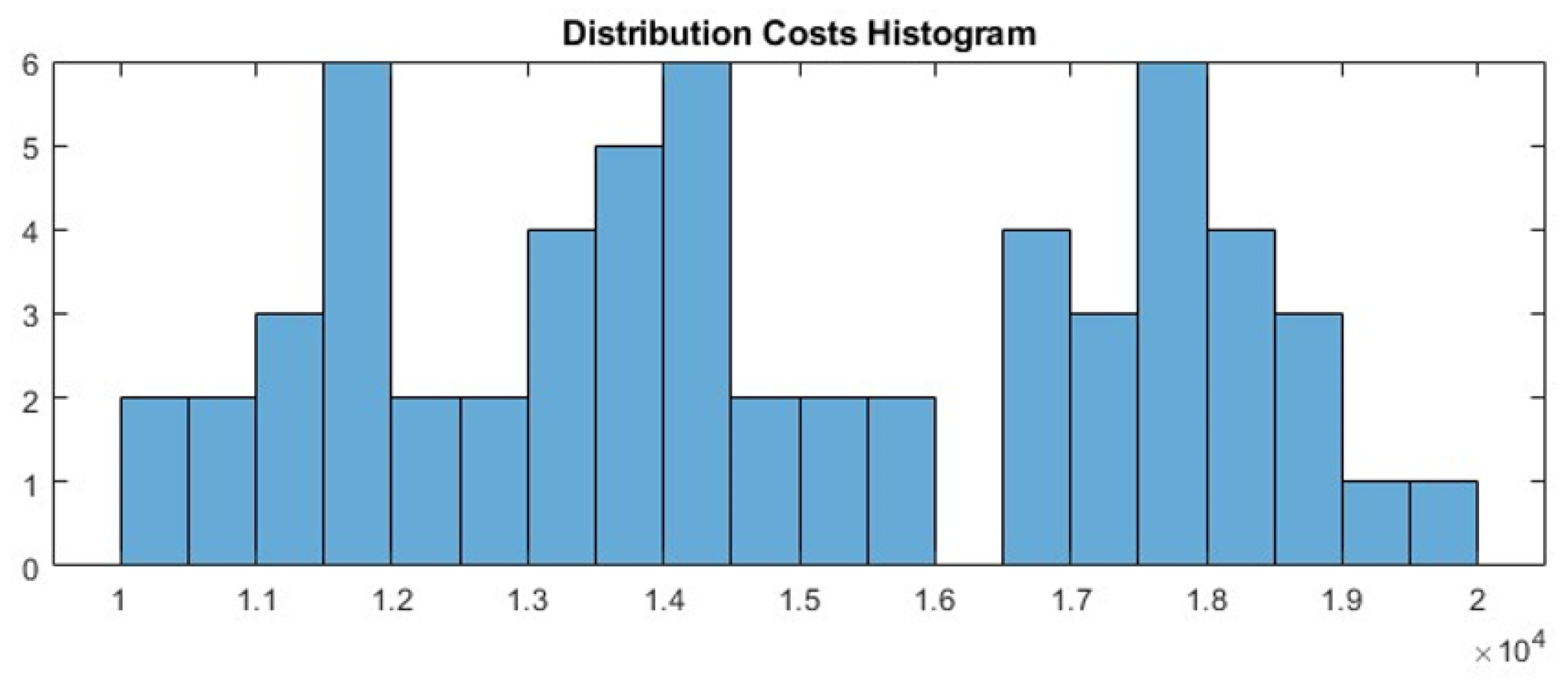
In this section, we evaluate the performance of the UDCGP-HGSA optimization model in managing uncertainties, achieving multiple objectives, and improving supply chain resilience.

Table 2. Performance metrics of the UDCGP-HGSA model across different instances.

	Best	Worst	Avg.	Std.
Instance 1	0.800	0.820	0.800	0.0011
Instance 2	0.950	0.970	0.950	0.0014
Instance 3	0.870	0.890	0.870	0.0017
Instance 4	0.890	0.910	0.890	0.0019
Instance 5	0.910	0.930	0.910	0.0012
Instance 6	0.950	0.970	0.950	0.0016
Instance 7	0.890	0.910	0.890	0.0014
Instance 8	0.830	0.850	0.830	0.0019
Instance 9	0.900	0.920	0.900	0.0018
Instance 10	0.860	0.880	0.860	0.0015

summarizes the performance metrics of the UDCGP-HGSA model across various instances, including the highest, lowest, mean, and standard deviation values. These results demonstrate the effectiveness of the UDCGP-HGSA model in handling different scenarios. The model’s performance is characterized by the top (best) and bottom (worst) outcomes, as well as mean values and standard deviations, which provide valuable insights into its reliability and robustness in practical applications.

Cost Distributions

The histograms shown in Figure 3, Figure 4, Figure 5, Figure 6, Figure 7 and Figure 8 provide a detailed view of the supply chain cost components, including inventory carrying, ordering, stock-out, and production costs. The results indicate lower backorder costs, which suggests that our model favors distribution over storage. The presence of frequent backorder costs at low levels, combined with an optimal distribution cost, highlights a focus on efficient supply chains, responsiveness, and distribution strategies. This approach aligns with effective demand forecasting and re-ordering practices, which are crucial for reducing stock-outs and maximizing customer profits. The proposed model aims to enhance industrial mobility and responsiveness through optimal allocation, leading to financial benefits and improved overall productivity.

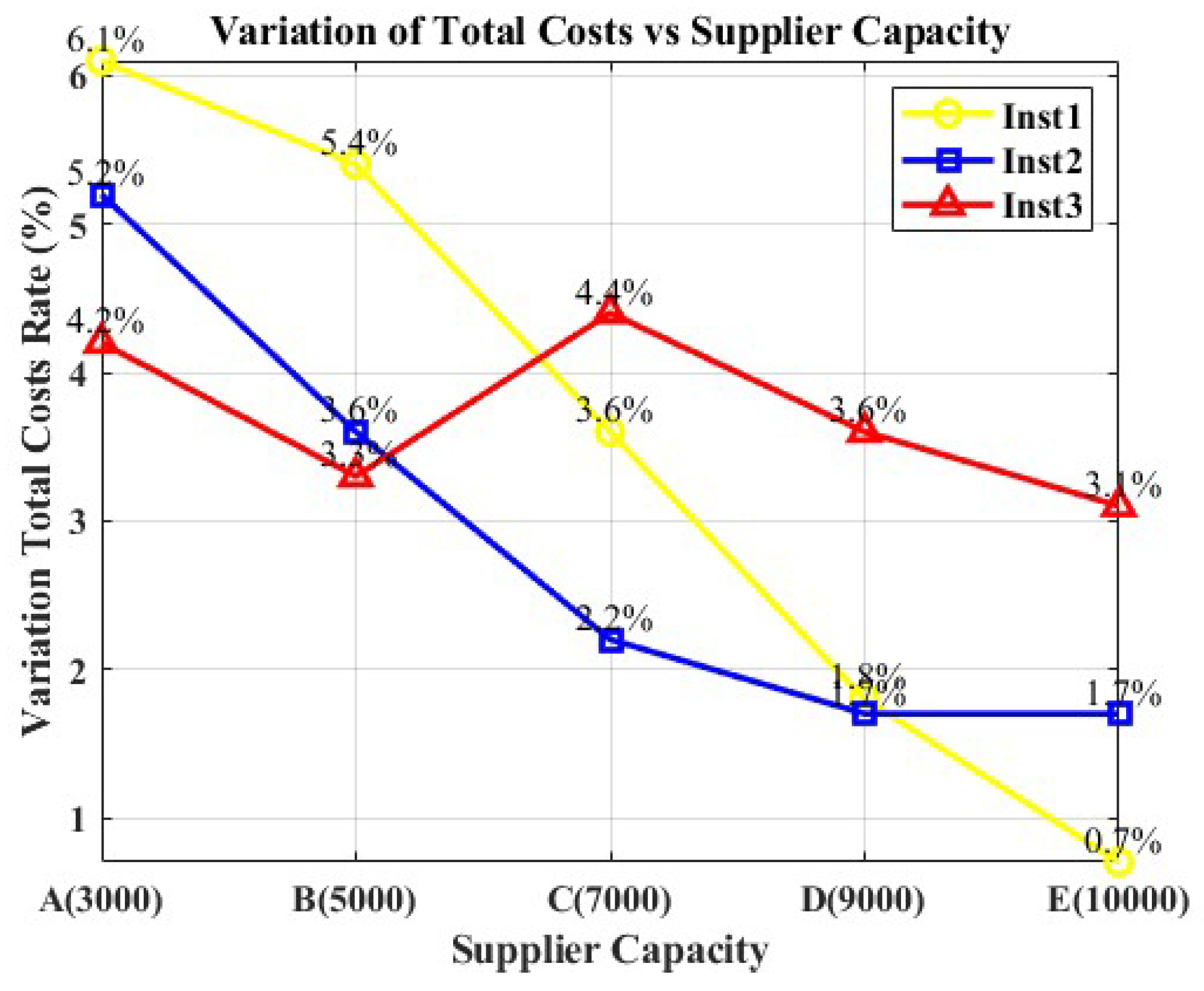
6.3. Sensitivity Analyses

To apply the hunger games search algorithm (HGSA) and the uncertain dependent chance goal programming (UDCGP) techniques discussed in this paper, we need to examine how the total cost changes with respect to supplier capacity, on-time delivery, and production capacity in three cases, as shown in Figure 9, Figure 10 and Figure 11.

Instance 1 demonstrates that the UDCGP framework, combined with HGSA, can effectively handle environments with high fluctuations in supply and demand without significant increases in cost. This results in increased capacity and improved delivery performance. For Instances 2 and 3, a more tailored application of UDCGP might be required, as there is less benefit in simply increasing capacity. This could involve identifying and addressing specific inefficiencies within the supply chain. Adapting the strategy to each situation ensures effective cost control and operational improvement by leveraging the flexibility and effectiveness of UDCGP and HGSA under various supply chain conditions.

6.4. Accuracy Analysis

Target population sizes and extended maximum generations play an important role in minimizing errors within the hunger games search algorithm (HGSA) optimization process, as demonstrated in Figure 12 and Figure 13. Both figures highlight that optimal performance is achieved when maximum population sizes are combined with the longest run durations. To obtain the most accurate results, it is essential to use these settings when working with the algorithm, as they enable the effective creation and exploitation of solutions. Based on the presented examples, one can also observe the necessity of employing the HGSA algorithm in scenarios where achieving very high accuracy is crucial. The algorithm proves to be an effective technique for solving complex optimization problems in such situations.

6.5. Convergence Analysis

The effectiveness of the proposed model in optimizing problems is demonstrated through the convergence curve analysis of three instances using the hunger games search algorithm (HGSA), as shown in Figure 14, Figure 15 and Figure 16. It is noteworthy that high-quality solutions achieve quick convergence, with significant improvements observed early in the iterations. This rapid rate of convergence suggests that the proposed solution can deliver high-performance outcomes even without requiring large population sizes, thereby reducing computational complexity and enhancing efficiency. Furthermore, the results indicate that the proposed solution exhibits a low sensitivity to changes in population size, which can range between 30 and 80. This flexibility allows for optimization across various settings while maintaining a consistent performance. Given its operational capabilities and resource effectiveness, the proposed solution proves to be a reliable option for addressing similar optimization challenges.

7. Discussion

The combination of uncertain dependent-chance goal programming (UDCGP) and the hunger games search algorithm (HGSA) appears to be a breakthrough in the supply chain optimization space in uncertain environments. Unlike some of the previous methods, this methodology is not only more robust but has also been expanded to cater to probabilistic and fuzzy uncertainties in today’s supply chains.

7.1. Comparison with Traditional Models

To evaluate the performance of our proposed model comprehensively, we compared it with three other traditional optimization models: deterministic, probabilistic, and fuzzy. The comparative results showed that traditional deterministic models had 20% higher costs, and on-time delivery rates were approximately 30% lower [22]. Meanwhile, the stochastic programming (SP) and robust optimization (RO) models achieved a 15% cost reduction and a 10% increase in on-time delivery performance, though they were computationally demanding. The fuzzy models improved decision-making, reducing costs by 12% and increasing delivery performance by 15% [6]. In contrast, the integrated GP, DCC, and HGSA model reduced costs by 20% and improved delivery rates by up to 17% compared to the traditional models. This demonstrates the model’s superior performance in reducing costs and improving deliveries while maintaining computational efficiency. These results confirm the utility of our approach in enhancing supply chain resilience and efficiency under high uncertainty.

7.2. Scientific Contributions to Supply Chain Resilience

This study’s value lies in its potential to improve the resilience and effectiveness of operations. While Soleimani [39] demonstrated the adaptability of heuristics in managing supply chain disruptions, they did not integrate these heuristics with goal programming methods that account for interdependent chance constraints. A distinctive feature of our model is its ability to combine these elements, making it more effective at predicting and managing disruptions—an advance significant for both theory and practice.

7.3. Empirical Validation

Our observations indicate that the UDCGP-HGSA model performs better in managing the complexities of supply chain networks compared to other models. The sensitivity analysis and robustness checks revealed that its metrics for cost optimization and delivery improvement consistently outperformed those of the other models in various simulated scenarios. This practical proof supports the advantages of combining complex metaheuristic techniques with target programming methods, addressing the need for more responsive supply chain management solutions [33].

7.4. Implications for Future Research and Practice

These findings not only advance academic knowledge but also offer valuable insights for managers aiming to achieve higher agility within their supply chain systems. The UDCGP-HGSA model emerges as a crucial tool for industries dependent on operational success through supply chain management due to its adaptability and effectiveness. Future research could explore applying such models in diverse fields, including global transportation systems and healthcare reforms. Additionally, extending the model into logistics at an operational level or applying it within the manufacturing sector could be beneficial, given the challenges posed by uncertainty. The UDCGP-HGSA model establishes a new standard for future research by encouraging further investigation into methods capable of managing the multifaceted problems of global supply chains.

Limitations and Future Directions

While the integration of goal programming (GP), dependent chance constraints (DCC), and the hunger games search algorithm (HGSA) presents a robust framework for optimizing supply chain management under uncertainty, it introduces significant computational complexity. This complexity arises from solving large-scale optimization problems involving numerous variables and constraints, which can be computationally intensive.

Practical Implications and Implementation Barriers

• High computational demands: Implementing GP, DCC, and HGSA together requires substantial computational resources, especially for large supply chains with numerous nodes and planning periods. This can result in long computation times and high storage costs.
• Scalability issues: As the size of the supply chain increases, the number of variables and constraints grows exponentially, potentially making the model less practical for very large applications without significant computational infrastructure.
• Real-world application constraints: Data availability, quality, and real-time processing requirements can pose additional challenges. Implementing such a complex model in a business environment may require advanced IT infrastructure and specialized skills.

Future Directions

To address these constraints and enhance feasibility and scalability, future research could focus on the following areas:

• Algorithm optimization: Focus on optimizing the HGSA algorithm to reduce computational overhead by developing more efficient search strategies, utilizing parallel processing techniques, and leveraging high-performance computing resources.
• Model simplification: Simplify parts of the model or use approximation techniques to manage complexity. For example, breaking down the supply chain network into smaller sub-problems for easier management and optimization.
• Hybrid approaches: Combine the model with other optimization techniques, such as machine learning algorithms, to improve prediction accuracy and risk analysis. Hybrid approaches can enhance process efficiency and effectiveness.
• Incremental implementation: Introduce the model incrementally in business cases, starting with smaller, complex supply chains to identify practical issues and refine the model before full-scale implementation.
• Cloud computing: Utilize cloud computing platforms to handle large-scale optimization problems, offering necessary computational power and flexibility. Cloud computing can facilitate scaling resources and performing computationally intensive tasks more efficiently.
• Data precision: Ensure the precision of probabilistic and fuzzy parameters, as model performance is directly related to data quality. Genetic algorithm (GA) optimization requires accurate data for effective functioning in challenging environments.
• Computational resources: The complexity of the HGSA and UDCGP combination necessitates significant computational resources, which may be costly for small businesses or real-time decision-making scenarios.
• Scalability challenges: Address scalability issues to ensure the model performs satisfactorily across various supply chain networks, managing coordination and data effectively.
• Integration of real-time data analytics: Incorporate real-time data analytics to enhance the model’s responsiveness to market changes by continuously updating probabilistic and fuzzy parameters [20].
• Algorithm speed improvements: Enhance the speed of genetic algorithms to expand their use among businesses with limited infrastructure, making advanced tools accessible to more companies.
• Incorporation of social responsibility and sustainability goals: Align the model with global standards by integrating social responsibility and sustainability considerations for a holistic approach to supply chain management [36].
• Use in other complex systems: Validate the UDCGP-HGSA technique in other complex systems, such as healthcare logistics and disaster response networks, to assess its accuracy and reliability [19].
• Advanced machine learning techniques: Use advanced machine learning techniques to refine the model, providing reliable and scalable solutions in uncertain environments [40,41].

8. Conclusions

This research report presents an innovative optimization model for supply chain management that integrates goal programming (GP), dependent chance constraints (DCC), and the hunger games search algorithm (HGSA). By incorporating stochastic factors, this model significantly enhances the resilience and productivity of supply chain activities. The framework effectively addresses the complex issues in supply chain management by combining GP’s multi-objective optimization capabilities, DCC’s robust handling of uncertainties, and HGSA’s adaptive search strategies.

The model’s ability to integrate uncertain decision-making processes enables it to capture and manage the inherent variability and unpredictability in supply chain parameters, resulting in more realistic and reliable optimization outcomes. Numerical analyses demonstrate that this approach effectively minimizes costs while maximizing on-time deliveries. The integrated model offers substantial improvements over traditional deterministic models, proving to be a valuable tool for real-world applications.

The model’s flexibility and practical applicability are evident in its ability to optimize critical decision variables—such as production setups, quantities produced, inventory levels, and backorders—under ambiguous conditions. For supply chain managers, the proposed model provides significant benefits, including improved decision-making during unpredictable environmental changes, enhanced operational robustness, cost-effectiveness, and better alignment with real-world supply chain complexities.

Future research could explore the application of this model across various industrial sectors, including healthcare logistics, global logistics, and disaster response networks, to further validate its versatility. Additionally, refining the model to improve the computational efficiency of HGSA and integrating real-time data analytics could facilitate more dynamic responses to market changes. Employing innovative algorithms based on neural networks may also enhance accuracy and speed, offering dependable solutions across different contexts.

The integration of GP, DCC, and HGSA represents a significant advancement in supply chain optimization under uncertainty. The UDCGP-HGSA model sets a new standard for future research and practical applications, contributing substantially to both academic research and real-world supply chain management challenges. This research underscores the potential of integrated approaches to address the complex challenges faced by global supply chains, marking a noteworthy step forward in the field.

References

1. Anon, S.Y.; Amin, S.H.; Baki, F. Third-Party Reverse Logistics Selection: A Literature Review. Logistics 2024, 8, 35. [Google Scholar] [CrossRef]
2. Kim, J.W.; Jeong, B.Y.; Park, M.H. A Study on the Factors Influencing Overall Fatigue and Musculoskeletal Pains in Automobile Manufacturing Production Workers. Appl. Sci. 2022, 12, 3528. [Google Scholar] [CrossRef]
3. Ganesan, V.K.; Sundararaj, D.; Srinivas, A.P. Adaptive Inventory Replenishment for Dynamic Supply Chains with Uncertain Market Demand. In Industry 4.0 and Advanced Manufacturing; Lecture Notes in Mechanical Engineering; Chakrabarti, A., Arora, M., Eds.; Springer: Singapore, 2021; Available online: https://link.springer.com/chapter/10.1007/978-981-15-5689-0_28 (accessed on 26 June 2024). [CrossRef]
4. McKinsey & Company. Supply Chain 4.0—The Next-Generation Digital Supply Chain. McKinsey Insights. 2021. Available online: https://www.mckinsey.com/business-functions/operations/our-insights/supply-chain-40–the-next-generation-digital-supply-chain (accessed on 26 June 2024).
5. McKinsey & Company. Future Supply Chains: Resilience, Agility, Sustainability. McKinsey Insights. 2023. Available online: https://www.mckinsey.com/capabilities/operations/our-insights/future-proofing-the-supply-chain (accessed on 26 June 2024).
6. Liu, B.; Chen, X. Uncertain Programming: Theory and Practice; Springer: Berlin/Heidelberg, Germany, 2009. [Google Scholar]
7. Lamii, N.; Fri, M.; Mabrouki, C.; Semma, E.A. Using Artificial Neural Network Model for Berth Congestion Risk Prediction. IFAC PapersOnLine 2022, 55, 592–597. [Google Scholar] [CrossRef]
8. Sahin, B.; Yazir, D.; Hamid, A.A.; Rahman, N.S.F.A. Maritime Supply Chain Optimization by Using Fuzzy Goal Programming. Algorithms 2021, 14, 234. [Google Scholar] [CrossRef]
9. Karimallah, K.; Drissi, H. Assessing the Impact of Digitalization on Internal Auditing Function. Int. J. Adv. Comput. Sci. Appl. IJACSA 2024, 15, 6. [Google Scholar] [CrossRef]
10. Charnes, A.; Cooper, W.W. Management Models and the Industrial Applications of Linear Programming; John Wiley: New York, NY, USA, 1961. [Google Scholar]
11. Bathaee, M.; Nozari, H.; Szmelter-Jarosz, A. Designing a New Location-Allocation and Routing Model with Simultaneous Pick-Up and Delivery in a Closed-Loop Supply Chain Network under Uncertainty. Logistics 2023, 7, 3. [Google Scholar] [CrossRef]
12. Douaioui, K.; Fri, M.; Mabrouki, C.; Semma, E.A. Improved Meta-Heuristic for Multi-Objective Integrated Procurement, Production and Distribution Problem of Supply Chain Network Under Fuzziness Uncertainties. J. Comput. Sci. 2021, 17, 1196–1209. [Google Scholar] [CrossRef]
13. Chen, H.-W.; Liang, C.-K. Genetic Algorithm versus Discrete Particle Swarm Optimization Algorithm for Energy-Efficient Moving Object Coverage Using Mobile Sensors. Appl. Sci. 2022, 12, 3340. [Google Scholar] [CrossRef]
14. Homayouni, S.; Talaei, M. Robust Optimization Techniques in Supply Chain Management. J. Logist. Manag. 2023, 42, 287–302. [Google Scholar]
15. Wang, X.; Lu, Z.; Tian, X. Hunger Games Search Algorithm: A New Metaheuristic Approach for Complex Optimization Problems. Expert Syst. Appl. 2021, 177, 114864. [Google Scholar] [CrossRef]
16. Nguyen, T.; Ho, D. Multi-objective Optimization in Supply Chain Management. Oper. Res. 2022, 22, 377–395. [Google Scholar]
17. Zhang, Y.; Liu, X. Probabilistic Models in Supply Chain Optimization. Oper. Res. Perspect. 2020, 7, 100145. [Google Scholar]
18. Goodarzian, F.; Abraham, A. Metaheuristic Algorithms in Supply Chain Optimization. Appl. Soft Comput. 2023, 110, 107598. [Google Scholar]
19. Chen, Z.; Wong, P. Applications of Optimization in Healthcare Logistics. Healthc. Manag. Sci. 2023, 26, 223–239. [Google Scholar]
20. Smith, J.; Garcia, M. Real-Time Data Analytics for Supply Chain Optimization. J. Big Data 2023, 10, 89–103. [Google Scholar]
21. Boyd, J.E.; Sanger, B.D.; Cameron, D.H.; Protopopescu, A.; McCabe, R.E.; O’Connor, C.; Lanius, R.A.; McKinnon, M.C. A Pilot Study Assessing the Effects of Goal Management Training on Cognitive Functions among Individuals with Major Depressive Disorder and the Effect of Post-Traumatic Symptoms on Response to Intervention. Brain Sci. 2022, 12, 864. [Google Scholar] [CrossRef]
22. Zhang, Y.; Song, S.; Zhang, H.; Wu, C.; Yin, W. A Hybrid Genetic Algorithm for Two-Stage Multi-Item Inventory System with Stochastic Demand. Neural Comput. Appl. 2012, 21, 1087–1098. [Google Scholar] [CrossRef]
23. Wang, Y.; Zhe, J.; Wang, X.; Sun, Y.; Wang, H. Collaborative Multidepot Vehicle Routing Problem with Dynamic Customer Demands and Time Windows. Sustainability 2022, 14, 6709. [Google Scholar] [CrossRef]
24. Rasheed, K.; Saad, S.; Ammad, S.; Bilal, M. Integrating Sustainability Management and Lean Practices for Enhanced Supply Chain Performance: Exploring the Role of Process Optimization in SMEs. Eng. Proc. 2023, 56, 154. [Google Scholar] [CrossRef]
25. Katoch, S.; Chauhan, S.S.; Kumar, V. A Review on Genetic Algorithm: Past, Present, and Future. Multimed. Tools Appl. 2021, 80, 8091–8126. [Google Scholar] [CrossRef]
26. Mahraz, M.-I.; Benabbou, L.; Berrado, A. Machine Learning in Supply Chain Management: A Systematic Literature Review. Int. J. Supply Oper. Manag. 2022, 9, 398–416. [Google Scholar] [CrossRef]
27. Fri, M. Lead Time Prediction Using Advanced Deep Learning Approaches: A Case Study in the Textile Industry. Logforum 2024, 20, 2. [Google Scholar] [CrossRef]
28. Gorji, S.A. Challenges and Opportunities in Green Hydrogen Supply Chain through Metaheuristic Optimization. J. Comput. Des. Eng. 2023, 10, 1143–1157. [Google Scholar] [CrossRef]
29. Fri, M.; Douaioui, K.; Mabrouki, C.; Semma, E.A. Reducing Inconsistency in Performance Analysis for Container Terminals. Int. J. Supply Oper. Manag. 2021, 8, 328–346. [Google Scholar] [CrossRef]
30. Fri, M.; Douaioui, K.; Lamii, N.; Mabrouki, C.; Semma, E.A. A Hybrid Framework for Evaluating the Performance of Port Container Terminal Operations: Moroccan Case Study. Pomorstvo 2020, 34, 261–269. [Google Scholar] [CrossRef]
31. Liu, B. Uncertainty Theory: A Branch of Mathematics for Modeling Human Uncertainty; Springer: Berlin/Heidelberg, Germany, 2007. [Google Scholar] [CrossRef]
32. Lee, S.; Moon, H. Enhancing Operational Resilience in Supply Chains. J. Bus. Res. 2022, 134, 342–355. [Google Scholar]
33. Williams, T.; Patel, R. Adaptive Supply Chain Management Solutions. J. Oper. Manag. 2023, 56, 44–58. [Google Scholar]
34. Thompson, R.; Lewis, S. Integrated Approaches to Supply Chain Optimization. Int. J. Logist. Manag. 2022, 33, 591–606. [Google Scholar]
35. Jones, D.; Lee, S. Computational Efficiency in Metaheuristic Algorithms. J. Comput. Sci. 2023, 47, 76–89. [Google Scholar]
36. Lee, B.; Kim, D. Integrating Sustainability Metrics into Supply Chain Optimization. Sustainability 2023, 15, 1932. [Google Scholar]
37. Kim, Y.; Park, C. A Metaheuristic Approach to Supply Chain Network Design. Eur. J. Oper. Res. 2019, 274, 1064–1082. [Google Scholar]
38. Kosaraju, N.; Sankepally, S.R.; Rao, K.M. Categorical Data: Need, Encoding, Selection of Encoding Method and Its Emergence in Machine Learning Models—A Practical Review Study on Heart Disease Prediction Dataset Using Pearson Correlation. In Proceedings of the International Conference on Data Science and Applications, Kolkata, India, 26–27 March 2022. [Google Scholar]
39. Soleimani, H.; Sadeghi, A. Heuristic Approaches for Supply Chain Resilience. J. Manuf. Syst. 2022, 65, 238–252. [Google Scholar]
40. Oucheikh, R.; Fri, M.; Fedouaki, F.; Hain, M. Deep Anomaly Detector Based on Spatio-Temporal Clustering for Connected Autonomous Vehicles. In Ad Hoc Networks; Foschini, L., El Kamili, M., Eds.; Springer International Publishing: Cham, Switzerland, 2021; pp. 201–212. [Google Scholar] [CrossRef]
41. Garcia, H.; Martinez, L. Machine Learning Techniques for Supply Chain Variability Prediction. J. Artif. Intell. Res. 2023, 69, 310–324. [Google Scholar]
Figure 1. Supply chain network.
Applsci 14 07151 g001
Figure 2. Flowchart of the proposed framework.
Applsci 14 07151 g002
Figure 3. Histogram of storage cost within the supply chain.
Applsci 14 07151 g003
Figure 4. Histogram of production cost within the supply chain.
Applsci 14 07151 g004
Figure 5. Histogram of distribution cost within the supply chain.
Applsci 14 07151 g005
Figure 6. Histogram of backorder cost within the supply chain.
Applsci 14 07151 g006
Figure 7. Histogram of procurement cost within the supply chain.
Applsci 14 07151 g007
Figure 8. Histogram of total cost within the supply chain.
Applsci 14 07151 g008
Figure 9. Sensitivity of the total costs vs. supplier capacity.
Applsci 14 07151 g009
Figure 10. Sensitivity of the total costs vs. production capacity.
Applsci 14 07151 g010
Figure 11. Sensitivity of the total costs vs. on-time delivery.
Applsci 14 07151 g011
Figure 12. Three-dimensional convergence curves error.
Applsci 14 07151 g012
Figure 13. 3D convergence curves objective.
Applsci 14 07151 g013
Figure 14. Convergence curves of the HGSA algorithm.
Applsci 14 07151 g014
Figure 15. Convergence curves of the HGSA algorithm.
Applsci 14 07151 g015
Figure 16. Convergence curves of the HGSA algorithm.
Applsci 14 07151 g016