Abstract
While machine learning methods have been successful in predicting air pollution, current deep learning models usually focus only on the time-based connection of air quality monitoring stations or the complex link between PM2.5 levels and explanatory factors. Due to the lack of effective integration of spatial correlation, the prediction model shows poor performance in PM2.5 prediction tasks. Predicting air pollution levels accurately over a long period is difficult because of the changing levels of correlation between past pollution levels and the future. In order to address these challenges, the study introduces a Convolutional Long Short-Term Memory (ConvLSTM) network-based neural network model with multiple feature extraction for forecasting PM2.5 levels in air quality prediction. The technique is composed of three components. The model-building process of this article is as follows: Firstly, we create a complex network layout with multiple branches to capture various temporal features at different levels. Secondly, a convolutional module was introduced to enable the model to focus on identifying neighborhood units, extracting feature scales with high spatial correlation, and helping to improve the learning ability of ConvLSTM. Next, the module for spatiotemporal fusion prediction is utilized to make predictions of PM2.5 over time and space, generating fused prediction outcomes that combine characteristics from various scales. Comparative experiments were conducted. Experimental findings indicate that the proposed approach outperforms ConvLSTM in forecasting PM2.5 concentration for the following day, three days, and seven days, resulting in a lower root mean square error (RMSE). This approach excels in modeling spatiotemporal features and is well-suited for predicting PM2.5 levels in specific regions.
1. Introduction
Fine particles (PM2.5) with a diameter of less than 2.5 μm are a major contributor to air pollution in cities [1,2,3,4,5]. Chronic exposure to high PM2.5 levels has been linked to negative effects on human organs and can possibly result in cardiovascular illnesses [3]. Prior research [3,6,7] identified two types of models, including a deterministic model and a statistical model, used to predict PM2.5 levels. Wang, W, Geng, G, and others predicted the concentration of PM2.5 using deterministic models by simulating the physical transport and chemical reactions of air pollutants [7]. Despite advancements in these methods, the high computational expenses and the unpredictability of the photochemical diffusion process and emissions prevent their use in assessing air quality over large areas [8]. The statistical model utilizes machine learning or deep learning technology to handle the complex connection between PM2.5 levels and external variables [9,10], achieving prediction accuracy comparable to deterministic models [11,12]. Statistical models are commonly used to forecast job outcomes due to their impressive efficiency, affordability, and expertise needed [10,13,14,15,16,17]. With the improvement of computer capabilities and deep learning principles, these statistical models have the potential to excel in forecasting PM2.5 levels, thus expanding their application in the field of atmospheric environmental science [9,10,18].
Nowadays, machine learning and deep learning models are extensively used to monitor and predict air pollutant levels. Some instances are the LSTM model for both long-term and short-term memory [7], the MLP model for multi-layer perceptron [19,20], the BPNN model for back propagation neural network [21], the SVR model for support vector regression [21,22], the RNN model for recurrent neural networks [23,24,25,26,27], and the SVR model for backpropagation neural networks. The LSTM model, along with GRNN, BPNN, and RNN, is considered one of the deep learning prediction models. The LSTM model, when configured for analyzing historical time series data, can capture temporal autocorrelation, making it a common choice for prediction tasks. The LSTM model is noteworthy for its ability to handle gradient inflation and error back propagation disappearance, as well as its effectiveness in capturing both long-term and short-term information. A number of LSTM-based models for forecasting air quality have been reported, including the Convolutional LSTM extension (C-LSTM) [6], by Mao [7] and others. To forecast 24-h PM2.5 concentration, a TS-LSTME model has been created using the basic LSTM model with sliding prediction [17], convolutional LSTM (GC-LSTM) [17], and depth multiple output LSTM (DM-LSTM) [28,29,30]. Both the CNN LSTM and the RLSTM are LSTMs. Convolutional neural networks (CNN) with self-attention mechanisms in 3D can improve the capacity to learn features in comparison to regular CNNs [31,32,33,34].
However, LSTM-based models have several key limitations in PM2.5 concentration prediction tasks. Several research studies have demonstrated the significant impact of spatiotemporal correlation on air pollution fluctuations [3,11,16,22,32]. Previous studies typically considered the temporal correlation of air pollution. Conversely, the models did not effectively integrate spatial correlation, leading to a decrease in predictive accuracy for PM2.5 concentration. Mao [11] introduced a TS-LSTME model that utilized conventional LSTM models and sliding prediction to forecast the 24-h PM2.5 levels in the Jinjingji region. In the meantime, convolutional LSTM and its different versions acquire spatial characteristics through the utilization of predetermined convolutional kernels and layers of stacked RNN layers. Its actual receptive field is still smaller than the theoretical receptive field, making it unable to effectively learn long-range spatial dependencies; other methods are insufficient in learning long-term time dependence. To overcome these issues, this paper proposes a multi-scale feature extraction neural network model based on the ConvLSTM network with convolutional long short-term memory for predicting PM2.5 concentration in air pollution prediction. Multiscale characteristics provide richer information than single-granularity characteristics. This article constructs a network with multiple branches to extract temporal features of PM2.5 with different granularities. The introduction of convolution helps memory cells capture long-term spatial dependencies.
2. Materials and Methods
2.1. Research Area and Data Source
China has made considerable strides toward reducing harmful pollution. However, the control of air pollution in some areas remains a problem. This study collected hourly historical PM2.5 concentrations from 30 air quality monitoring stations in the Jilin Province from 1 January 2016 to 31 December 2022. PM2.5 concentration data were obtained from the national urban air quality real-time platform (http://www.weather.com.cn/ (accessed on 1 March 2024)) and meteorological data service center (http://data.cma.cn/en (accessed on 1 March 2024)). The adjacent short-term values interpolate the missing PM2.5 concentration data to verify the proposed model’s performance.
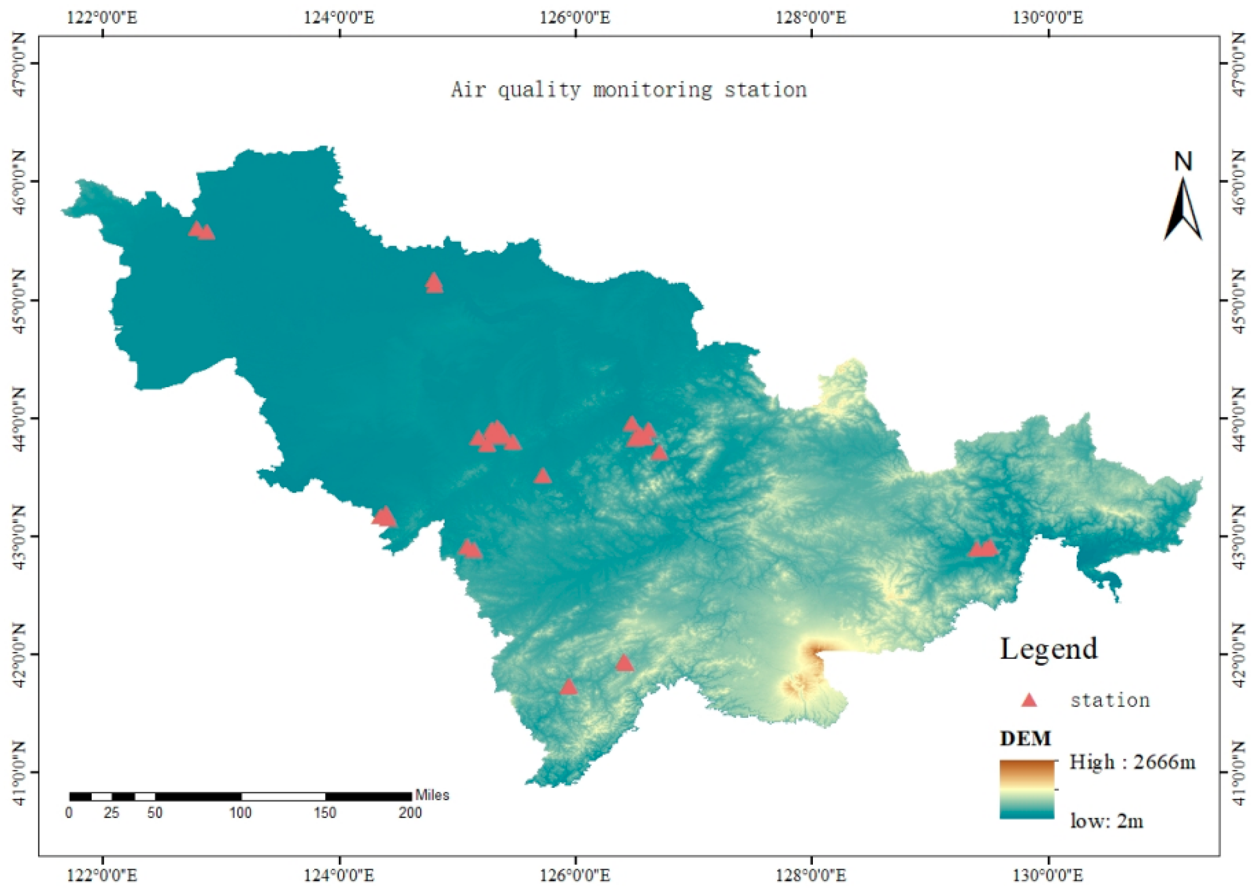
Two distinct types of information are included in our sample, (a) the geographical locations of all monitoring stations and (b) PM2.5 concentration data over time for each monitoring location. By using inverse distance weighted (IDW) interpolation, pollution data were matched to air quality monitoring stations. Figure 1 displays the study area and positions of the 30 air quality monitoring stations, while Table 1 presents the statistical data for these sites in the Jilin province.

Figure 1.
The study region along with the 30 stations for monitoring air quality.

Table 1.
Data set.
2.2. Regional Space Station Representation and Data Conversion
We developed a PM2.5 forecasting model utilizing a fusion of multiple time scales and regional space station representation and data conversion. Due to the uneven distribution of the 30 air quality monitoring stations in Jilin Province, the network is unable to use these irregular images as input.
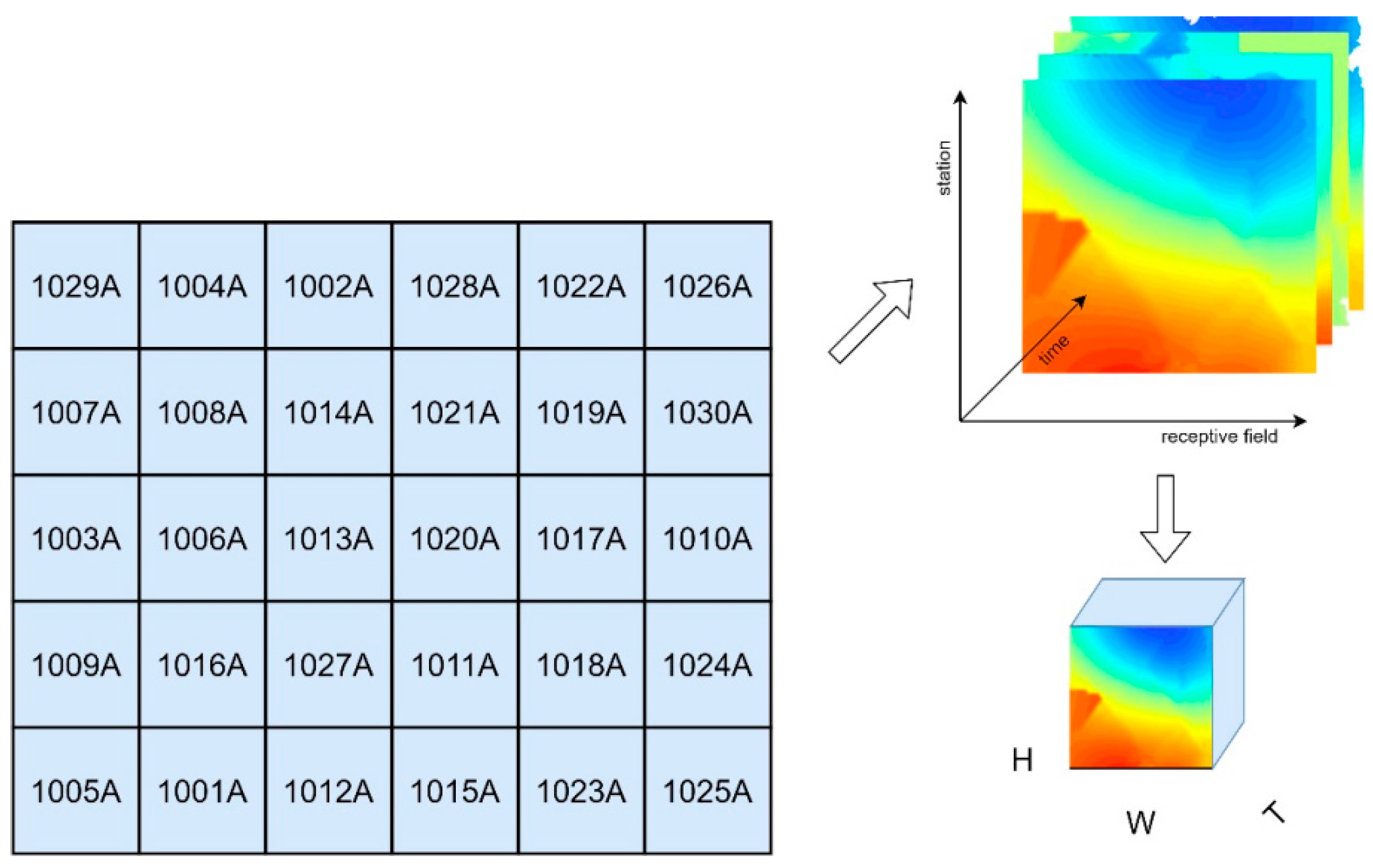
Considering Tobler’s first geographical law [3], the study area is segmented into discrete square or rectangular pixels arranged on a grid using a raster dataset to represent the location features of meteorological stations. A regional space station representation method is used to reorganize 30 air quality monitoring stations into a regular distribution and positional relationships (longitude and latitude) are used to adapt to the data input requirements of the ConvLSTM network, which is considered an approximate representation of the regional PM2.5 co. The codes in the blocks in the figure represent the numbering names of the 30 air quality monitoring stations. Figure 2 shows the reorganization and distribution of 30 air quality monitoring stations and their concentration distribution.

Figure 2.
Layout of 30 air quality monitoring stations in Jilin Province.
In the process of data conversion, we first define a space-time matrix of pollution in a given area. In the matrix Xt RH*W, H and W represent the proportional vertical and horizontal dimensions of the surveillance region, which can be thought of as the area PM2.5 approximate representation of the concentration distribution. We also represent the pollution map at time t by accommodating the positional relationship (longitude and latitude) data input requirements of the multi-branch network. It is assumed that the data at time t is Xt ∈ RH*W and the spatiotemporal series <X1, X2, …> ∈ RS*H*W includes numerous continuous frames of pollution images; S is the temporal depth, and at time t, the forecasting model predicts the most probable future sequence of K steps <Xt+1, …, Xt+k>.
2.3. Multi-Scale Feature Extraction
The primary goals of the initial phase involve establishing the spatiotemporal relationships among air quality monitoring stations and incorporating them into the model input matrix. The PM2.5 concentration at the appropriate location in space at time t, which is the matrix of WH, can be written as the input of our network as a matrix, Xt ∈ RH*W. Our model receives its input from a spatiotemporal matrix of contaminants that was created in chronological order. The time interval between two time points on the axis can be denoted as Ts, e, and l, where Ts is the starting point and e is the ending point, with e being greater than s. Additionally, l is the time granularity of the time granule, that is, the number of time points contained in Ts, e, l. Different lengths of PM2.5 data need to be generated prior to extracting PM2.5 temporal characteristics at different levels. We change the sliding window’s size to produce PM2.5 data of various lengths.
As seen in Figure 3, we create a network with numerous branches, each of which is capable of extracting temporal information at various sizes. Multi-scale features contain a greater amount of information compared to single-scale features. H*W is a matrix with dimensions of H and W, where * represents matrix multiplication. The multi-granularity feature method for predicting PM2.5 offers benefits in enhancing accuracy and overall performance.
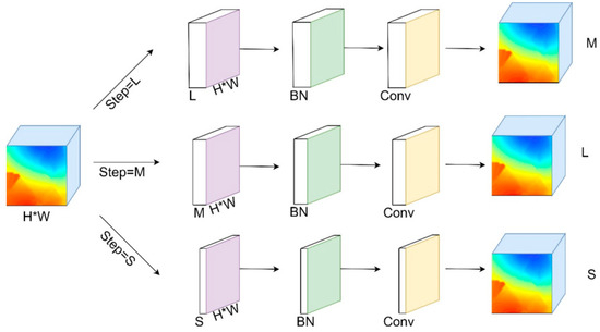
Figure 3.
Multi-branch network architecture.
Each branch in the multi-grain feature extractor has the same structure. The convolution method captures the characteristics of different regions while preserving spatial details of PM2.5. Various network branches can extract features of different sizes. One of the scale feature sequences can be written as Sn = [Sn + 1, Sn + 2,…, Sn + k] if the extraction process begins on day n.
2.4. ConvLSTM
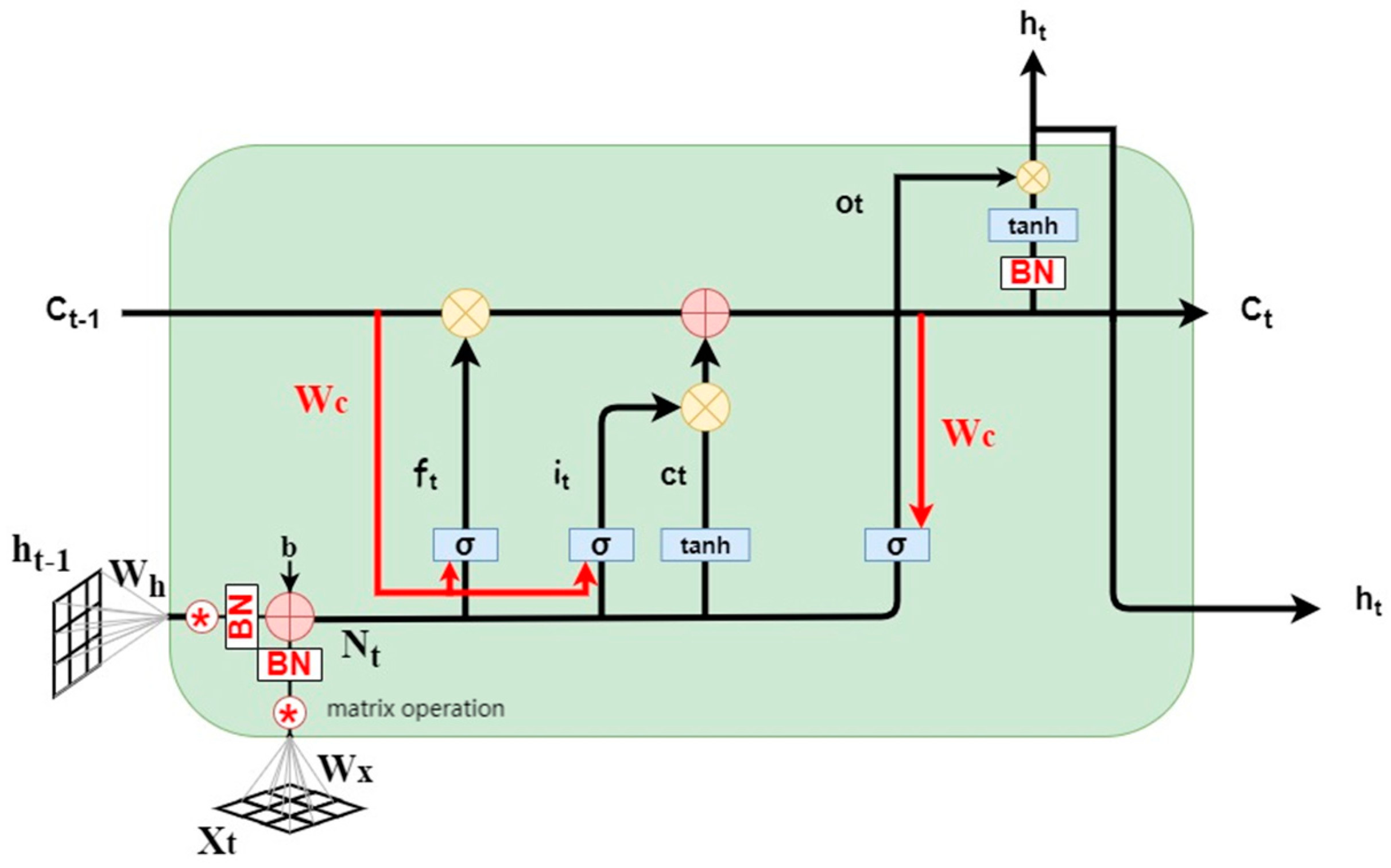
The ConvLSTM network enhances the traditional LSTM model by incorporating convolution operations, allowing it to capture both temporal and spatial correlations among air quality monitoring stations, thereby extracting intricate spatiotemporal correlation features related to air pollution. The structure is shown in Figure 4.

Figure 4.
ConvLSTM structure diagram.
The classic LSTM model is limited to capturing the temporal relationship of just one air quality monitoring station. The ConvLSTM network enhances traditional LSTM models by incorporating convolutional operations, similar to LSTM models, to capture temporal correlations and CNN to capture spatial correlations among air quality monitoring stations, ultimately extracting intricate spatiotemporal correlation features of air pollution (Figure 3) [35]. Furthermore, ConvLSTM networks are able to address the issues of gradient explosion and vanishing during error backpropagation, allowing for improved capture of long-term, short-term, and neighboring information compared to conventional LSTM networks. Similar to LSTM networks, ConvLSTM networks also provide information transmission through forget gates ft, input gates it, and output gates ot. Xt, Ct, and ht represent the input, internal, and external conditions at a specific time. The forget gate ft, input gate it, and output gate ot are determined using convolution and batch normalization, along with internal Ct−1 or Ct based on states Xt and ht−1. ConvLSTM networks outperform traditional LSTM models in capturing long-term information dependencies. The information transmission formula in the ConvLSTM network is as follows:
Nt is the middle variable of the input feature at the present time t computed by convolution; Wx and Wh are the weight matrices of Nt; BN is for batch normalization; Wci and Wcm are the weight matrices for variables connecting Ct−1 and input gate it and Ct−1 and forget gate ft; Wco is the weight matrix for variables connecting internal Ct and output gate it; BN, bi, bf, bc, and bo are the respective biases; and ◦ represents matrix operations.
The model is developed using multi-grain features to forecast PM2.5. This model consists of various branches, and the final prediction is generated by combining the results from these branches. The process of fusion is described as follows:
M signifies the number of branches. The forecasted outcome for the i-th division can be denoted as Pi. The final prediction is expressed in Pfusion.
3. Results
3.1. Experimental Data and Environment
Data were gathered in Jilin from 1 January 2016 to 31 December 2021 through the National Urban Air Quality Real-time Publishing Platform (is: http://www.weather.com.cn/; accessed in 1 March 2022). Thirty air quality monitoring stations’ historical hourly PM2.5 values are used to confirm the effectiveness of the suggested model. The missing PM2.5 concentration data are interpolated using nearby short-term values. PM2.5 data from 2016 to 2019 are used in the training. Following the training of the model’s parameters, PM2.5 data from the years 2020 and 2021 were utilized as a validation set to assess the effectiveness of the predictive model. Tensorflow and Keras are two of the packages utilized in the model creation, and Python is used for all method executions.
3.2. Evaluation Index
The PM2.5 prediction theory adopted in this paper can be regarded as a regression modeling problem. Therefore, statistically-based regression analysis metrics can effectively evaluate the performance of all models. This paper uses MAE (mean absolute error) and RMSE as classic statistical indicators. It is defined as follows:
where y-pred is the predicted value, y-true is the true value, and N is the number of samples.
3.3. Determination of Network Structure
Different scales of characteristics can be extracted from the structure of many branches. The variance of characteristics gradually diminishes as the number of model branches rises, which lowers prediction precision. In order to identify the network topology, a network comparison experiment with several branches is created and its RMSE and MAE are compared. Our method is executed five times independently with identical settings to minimize the influence of network initialization on the prediction outcomes, and the final result is calculated based on the average value. The prediction accuracy of time series models usually decreases with the increase of time. We observe the prediction results of the model for the next day, three days, and seven days to verify its performance in short-term, medium-term, and long-term prediction tasks.
In Table 2, the RMSE and MAE values for predicting PM2.5 levels one, three, and seven days ahead are displayed for a network with multiple branches. During the specified dates, it was found that the root mean square error (RMSE) and mean absolute error (MAE) of the prediction outcomes based on multi-scale features were lower compared to the RMSE and MAE of single-scale features. This distinction implies that multiscale characteristics may enhance PM2.5 forecast precision. The explanation might be that multi-scale characteristics represent various PM2.5 fluctuation patterns and can thus give more accurate information for PM2.5 prediction.
Table 2.
Prediction results with different structures.
Additionally, the network with three branches has the lowest RMSE and MAE during the next one, three, and seven days.
This study shows that networks with three branches perform better than those with two and four branches. Table 2 displays the RMSE and MAE of PM2.5 prediction results for one, three, and seven days ahead when the network is extensive. The root mean square error (RMSE) and mean absolute error (MAE) for the multi-scale forecast on the selected dates were determined to be less than the single-scale forecast results.
3.4. Input Length Analysis and Fusion Policy
The variations in input length can lead to changes in the PM2.5 patterns shown in each window, potentially impacting the forecast model’s accuracy. In the experimental setup, four distinct combinations of lengths were utilized as inputs for forecasting PM2.5 levels on the second, third, and seventh days. Subsequently, RMSE values were compared to identify the optimal input length.
In Table 3, there is a comparison of RMSEs for forecast results of the next day, three days, and seven days based on various input lengths. For projects with ‘forecast day = 1’, the RMSEs for the total input lengths of 4, 8, and 12 were less than the RMSEs for the remaining three combinations. Hence, this particular input mix is appropriate for forecasting PM2.5 levels for the next day. The RMSE for the third combination, where the predicted days were set to 3, was 0.4225, indicating the superior performance among the four length combinations.
Table 3.
Results of predictions with varying input lengths.
Hence, a mix of 12, 15, and 18 has been chosen to forecast PM2.5 levels for the upcoming three days. The lowest prediction error for PM2.5 over the next week was achieved by combining time intervals of 28, 35, and 42 days out of four different combinations. Hence, the mixture is utilized in forecasting PM2.5 levels for the upcoming week.
3.5. Comparison with Other Methods
SVR, LSTM, LSTME, T-LSTME, and ConvLSTM are some popular models. This article selects these models to compare with the proposed models to evaluate their performance. LSTME and TS-LSTME models consider past hourly PM2.5 levels, daily meteorological information, geographic factors, and human behavior, but do not factor in air quality monitoring. MLR, SVR, and LSTM models consider only past hourly PM2.5 levels. ConvLSTM has some capacity to extract the spatial–temporal connection from the spatial correlation between stations. The performance of each approach is evaluated by comparing the RMSE and MAE of the predicted results.
Table 4 demonstrates that ConvLSTM and the novel approach presented in this study outperform SVR, LSTM, and LSTME in forecasting PM2.5 levels. The significance of spatial correlation in PM2.5 prediction is underscored by this finding. Additional analysis of RMSE and MAE reveals that the proposed model has a lower prediction error compared to ConvLSTM, primarily because ConvLSTM lacks adequate modeling capabilities and struggles to capture long-range spatial correlations with fixed convolution kernels.
Table 4.
Prediction results of different models.
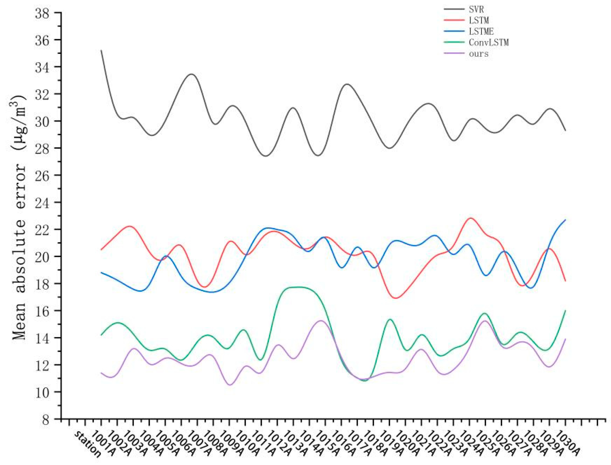
In Figure 5, We display the daily performance (MAE) of several models for 30 air quality monitoring sites in the province of Jilin. The outcomes demonstrate that the suggested model outperforms the SVR, LSTM, LSTME, and ConvLSTM models. The proposed model performs better than the ConvLSTM model in terms of accuracy at the majority of air quality monitoring locations.
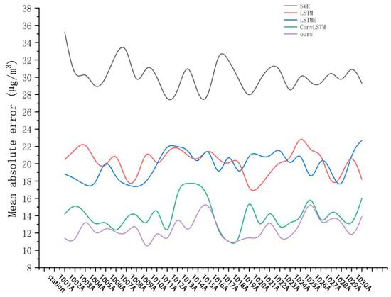
Figure 5.
Comparison of Model MAE Errors.
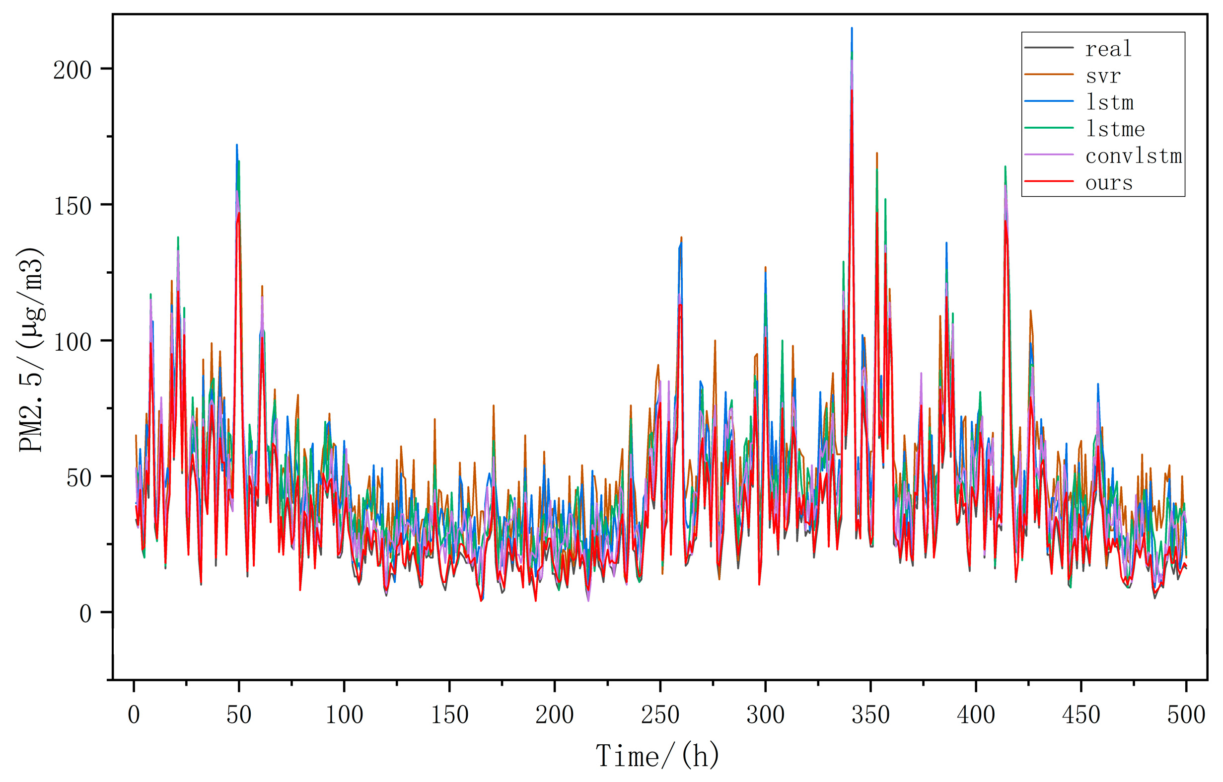
We choose the predicted data from the 1001A station for presentation from 26 February 2022 to 18 March 2022 to present the findings in an understandable manner. Gray represents the actual data value, while brown, blue, green, purple, and red represent the projected or predicted values from the different models used in this study. The data visualizations clearly show that while the prediction accuracy of the other two models aligns well with the actual data when the prediction interval is small, the model introduced in this study outperforms them in terms of accuracy. Simultaneously, the model presented in this study also surpasses the other two models in peak forecasting performance. Figure 6, Figure 7 and Figure 8 show that the longer the forecast period, the lower the accuracy of predicting peak values and future trends for each model. At a 7-day prediction time step, the forecast patterns of LSTM and ConvLSTM begin to diverge from the real data, evident in the predicted values from 100 to 200 h in Figure 8. The projected outcomes and upcoming patterns of the model discussed in this article may align more closely with the real data. Hence, the model presented in this study is capable of more accurately predicting PM2.5 levels over an extended period of time.
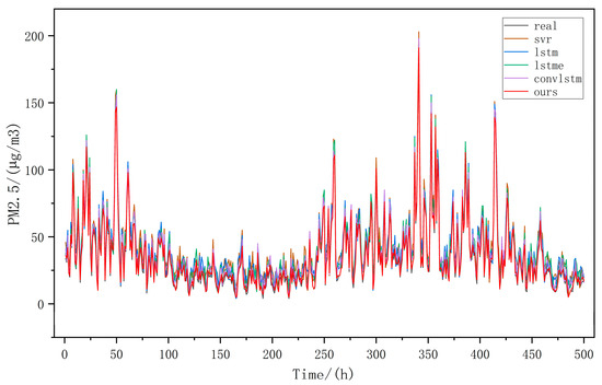
Figure 6.
Forecast outcomes from the three techniques over a 1-day prediction interval with MAE Errors. Comparison of prediction results of different models within 1-day prediction interval.
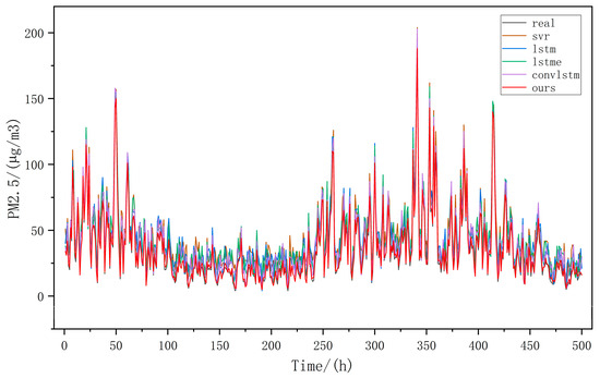
Figure 7.
Forecast outcomes from the three techniques over a 3-day prediction interval with MAE errors. Comparison of prediction results of different models within 3-day prediction interval.
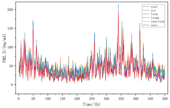
Figure 8.
Forecast outcomes from the three techniques over a 7-day prediction interval with MAE Errors. Comparison of prediction results of different models within 7-day prediction interval.
4. Conclusions
Forecasting the levels of PM2.5 is crucial for both individuals’ daily routines and environmental management. This paper suggests a fusion model that combines information from features at different spatiotemporal scales, considering their diverse effects on prediction outcomes. We evaluated our network on real-world datasets and experimental results showed that our model achieved state-of-the-art results. Our proposed model outperforms other models in the figures and tables, primarily because multi-granularity features offer richer temporal granularity and can capture more complex PM2.5 variations compared to single-granularity features. In upcoming projects, we plan to investigate methods for resolving the challenge of declining accuracy in predictions as time progresses. One idea is to use stochastic neural networks to model uncertainty and improve predictive performance. Furthermore, we will also try to conduct convolution computations in the frequency realm in order to accelerate the training procedure.
Author Contributions
Conceptualization, Y.S. and P.W.; methodology, S.L.; software, S.L. All authors have read and agreed to the published version of the manuscript.
Funding
This research is supported by grants from the Scientific Research Program of the Jilin Provincial Department of Education [JJKH20240424KJ http://jyt.jl.gov.cn (accessed on 1 June 2024)].
Institutional Review Board Statement
Not applicable.
Informed Consent Statement
Not applicable.
Data Availability Statement
The original contributions presented in the study are included in the article, further inquiries can be directed to the corresponding author.
Conflicts of Interest
The authors declare no conflicts of interest.
References
- Barzeghar, V.; Sarbakhsh, P.; Hassanvand, M.S.; Faridi, S.; Gholampour, A. Long-term trend of ambient air PM10, PM2.5, and O3 and their health effects in Tabriz city, Iran, during 2006–2017. Sustain. Cities Soc. 2020, 54, 101988. [Google Scholar] [CrossRef]
- Kampa, M.; Castanas, E. Human health effects of air pollution. Environ. Pollut. 2008, 151, 362–367. [Google Scholar] [CrossRef] [PubMed]
- Wang, W.; Zhao, S.; Jiao, L.; Taylor, M.; Zhang, B.; Xu, G.; Hou, H. Estimation of PM2.5 concentrations in china using a spatial back propagation neural network. Sci. Rep. 2019, 9, 13788. [Google Scholar] [CrossRef] [PubMed]
- National Urban Air Quality Report of China. 2019. Available online: https://www.mee.gov.cn/hjzl/dqhj/cskqzlzkyb/202001/P020200115538458118358.pdf (accessed on 2 July 2019).
- Li, T.; Shen, H.; Zeng, C.; Yuan, Q.; Zhang, L. Point-Surface Fusion of station measurements and satellite observations for mapping PM2.5 distribution in China: Methods and assessment. Atmos. Environ. 2017, 152, 477–489. [Google Scholar] [CrossRef]
- Wen, C.; Liu, S.; Yao, X.; Peng, L.; Li, X.; Hu, Y.; Chi, T. A novel spatiotemporal convolutional long short-term neural network for air pollution prediction. Sci. Total Environ. 2019, 654, 1091–1099. [Google Scholar] [CrossRef] [PubMed]
- Geng, G.; Zhang, Q.; Martin, R.V.; van Donkelaar, A.; Huo, H.; Che, H.; Lin, J.; He, K. Estimating long-term PM2.5 concentrations in China using satellite-based aerosol optical depth and a chemical transport model. Remote Sens. Environ. 2015, 166, 262–270. [Google Scholar] [CrossRef]
- Wang, W.; Jiao, L.; Zhao, S.; Liu, A. Modeling air quality prediction using a deep learning approach: Method optimization and evaluation. Sustain. Cities Soc. 2020, 65, 102567. [Google Scholar]
- Li, T.; Shen, H.; Yuan, Q.; Zhang, L. Geographically and temporally weighted neural networks for satellite- Based mapping of ground-level PM2.5. ISPRS J. Photogramm. Remote Sens. 2020, 167, 178–188. [Google Scholar] [CrossRef]
- Yuan, Q.; Shen, H.; Li, T.; Li, Z.; Li, S.; Jiang, Y.; Xu, H.; Tan, W.; Yang, Q.; Wang, J.; et al. Deep learning in environmental remote sensing: Achievements and challenges. Remote Sens. Environ. 2020, 241, 111716. [Google Scholar] [CrossRef]
- Lv, B.; Cai, J.; Xu, B.; Bai, Y. Understanding the rising phase of the PM2.5 concentration evolution in large China cities. Sci. Rep. 2017, 7, 46456. [Google Scholar] [CrossRef]
- Gupta, P.; Christopher, S.A. Particulate matter air quality assessment using integrated surface, satellite, and meteorological products: 2. A neural network approach. J. Geophys. Res. Atmos. 2009, 114, D20205. [Google Scholar] [CrossRef]
- Zhang, G.; Lu, H.; Dong, J.; Poslad, S.; Li, R.; Zhang, X.; Rui, X. A Framework to predict high-resolution spatiotemporal PM2.5 distributions using a deep-learning Model: A case study of Shijiazhuang, China. Remote Sens. 2020, 12, 2825. [Google Scholar] [CrossRef]
- Fan, Z.; Zhan, Q.; Yang, C.; Liu, H.; Bilal, M. Estimating PM2.5 concentrations using Spatially local xgboost based on full-covered Sara aod at the urban scale. Remote Sens. 2020, 12, 3368. [Google Scholar] [CrossRef]
- Shen, H.; Jiang, Y.; Li, T.; Cheng, Q.; Zeng, C.; Zhang, L. Deep learning-based air temperature mapping by fusing remote sensing, station, simulation and socioeconomic data. Remote Sens. Environ. 2020, 240, 111692. [Google Scholar] [CrossRef]
- Wan, R.; Mei, S.; Wang, J.; Liu, M.; Yang, F. Multivariate temporal convolutional network: A deep neural networks approach for multivariate time series forecasting. Electronics 2019, 8, 876. [Google Scholar] [CrossRef]
- Qi, Y.; Li, Q.; Karimian, H.; Liu, D. A hybrid model for spatiotemporal forecasting of PM2.5 based on graph convolutional neural network and long. Sci. Total Environ. 2019, 664, 1–10. [Google Scholar] [CrossRef]
- Shen, H.; Li, T. Progress of remote sensing mapping of atmospheric PM2.5. Acta Geod. Cartogr. Sin. 2019, 48, 1624–1635. [Google Scholar]
- Han, L.; Zhao, J.; Gao, Y.; Gu, Z.; Xin, K.; Zhang, J. Spatial distribution characteristics of PM2.5 and PM10 in Xi’an city predicted by land use regression models. Sustain. Cities Soc. 2020, 61, 102329. [Google Scholar] [CrossRef]
- Stadlober, E.; Hormann, S.; Pfeiler, B. Quality and performance of a PM10 daily forecasting model. Atmos. Environ. 2008, 42, 1098–1109. [Google Scholar] [CrossRef]
- Perez, P.; Reyes, J. An integrated neural network model for PM10 forecasting. Atmos. Environ. 2006, 40, 2845–2851. [Google Scholar] [CrossRef]
- Suarez Sanchez, A.; Garcia Nieto, P.J.; Riesgo Fernandez, P.; Del Coz Diaz, J.J.; Iglesias-Rodriguez, F.J. Application of an SVM-based regression model to the air quality study at local scale in the Aviles urban area (Spain). Math. Comput. Model. 2011, 54, 1453–1466. [Google Scholar] [CrossRef]
- Schneider, R.; Vicedo-Cabrera, A.M.; Sera, F.; Masselot, P.; Stafoggia, M.; de Hoogh, K.; Kloog, I.; Reis, S.; Vieno, M.; Gasparrini, A. A satellite-based spatio-temporal machine learning model to reconstruct daily PM2.5 concentrations across Great Britain. Remote Sens. 2020, 12, 3803. [Google Scholar] [CrossRef] [PubMed]
- Abirami, S.; Chitra, P. Regional air quality forecasting using spatiotemporal deep learning. J. Clean. Prod. 2021, 283, 125341. [Google Scholar] [CrossRef]
- Zhang, B.; Zou, G.; Qin, D.; Lu, Y.; Jin, Y.; Wang, H. A novel Encoder-Decoder model based on read-first LSTM for air pollutant prediction. Sci. Total Environ. 2021, 765, 144507. [Google Scholar] [CrossRef] [PubMed]
- Ma, J.; Ding, Y.; Cheng, J.C.P.; Jiang, F.; Gan, V.J.L.; Xu, Z. A Lag-FLSTM deep learning network based on Bayesian optimization for multi-sequential-variant PM2.5 prediction. Z. A lag-FLSTM deep learning network based on bayesian optimization for multi-sequential-variant PM2.5 prediction. Sustain. Cities Soc. 2020, 60, 102237. [Google Scholar] [CrossRef]
- Yan, R.; Liao, J.; Yang, J.; Sun, W.; Nong, M.; Li, F. Multi-hour and multi-site air quality index forecasting in Beijing using CNN, LSTM, CNN-LSTM, and spatiotemporal clustering. Expert Syst. Appl. 2021, 169, 114513. [Google Scholar] [CrossRef]
- Leng, X.; Wang, J.; Ji, H.; Wang, Q.; Li, H.; Qian, X.; Li, F.; Yang, M. Prediction of size-fractionated airborne particle-bound metals using MLR, BP-ANN and SVM analyses. Chemosphere 2017, 180, 513–522. [Google Scholar] [CrossRef] [PubMed]
- Li, X.; Peng, L.; Yao, X.; Cui, S.; Hu, Y.; You, C.; Chi, T. Long short-term memory neural network for air pollutant concentration predictions: Method development and evaluation. Environ. Pollut. 2017, 231, 997–1004. [Google Scholar] [CrossRef] [PubMed]
- Zhou, Y.; Chang, F.; Chang, L.; Kao, I.; Wang, Y. Explore a deep learning multi-output neural network for regional multi-step-ahead air quality forecasts. J. Clean. Prod. 2019, 209, 134–145. [Google Scholar] [CrossRef]
- Huang, C.; Kuo, P. A deep CNN-LSTM model for particulate matter (PM2.5) forecasting in Smart Cities. Sensors 2018, 18, 2220. [Google Scholar] [CrossRef]
- Li, T.; Shen, H.; Yuan, Q.; Zhang, X.; Zhang, L. Estimating ground-level PM2.5 by fusing satellite and station observations: Zhang, L. Estimating ground-level PM2.5 by fusing satellite and station observations:A geo-intelligent deep learning approach. Geophys. Res. Lett. 2017, 44, 11,985–11,993. [Google Scholar] [CrossRef]
- Li, T.; Wang, Y.; Yuan, Q. Remote sensing estimation of regional NO2 via space-time neural networks. Remote Sens. 2020, 12, 2514. [Google Scholar] [CrossRef]
- Tran, D.; Bourdev, L.; Fergus, R.; Torresani, L.; Paluri, M. Learning spatiotemporal features with 3D convolutional networks. In Proceedings of the IEEE International Conference on Computer Vision, Santiago, Chile, 7–13 December 2015; pp. 4489–4497. [Google Scholar] [CrossRef]
- Luo, W.; Li, Y.; Urtasun, R.; Zemel, R. Understanding the effective receptive field in deep convolutional neural networks. In Proceedings of the 30th International Conference on Neural Information Processing Systems (NIPS), Barcelona, Spain, 5–10 December 2016; pp. 4905–4913. [Google Scholar]


Disclaimer/Publisher’s Note: The statements, opinions and data contained in all publications are solely those of the individual author(s) and contributor(s) and not of MDPI and/or the editor(s). MDPI and/or the editor(s) disclaim responsibility for any injury to people or property resulting from any ideas, methods, instructions or products referred to in the content. |
© 2024 by the authors. Licensee MDPI, Basel, Switzerland. This article is an open access article distributed under the terms and conditions of the Creative Commons Attribution (CC BY) license (https://creativecommons.org/licenses/by/4.0/).