A Robust and Efficient Method for Effective Facial Keypoint Detection

Abstract

Facial keypoint detection technology faces significant challenges under conditions such as occlusion, extreme angles, and other demanding environments. Previous research has largely relied on deep learning regression methods using the face’s overall global template. However, these methods lack robustness in difficult conditions, leading to instability in detecting facial keypoints. To address this challenge, we propose a joint optimization approach that combines regression with heatmaps, emphasizing the importance of local apparent features. Furthermore, to mitigate the reduced learning capacity resulting from model pruning, we integrate external supervision signals through knowledge distillation into our method. This strategy fosters the development of efficient, effective, and lightweight facial keypoint detection technology. Experimental results on the CelebA, 300W, and AFLW datasets demonstrate that our proposed method significantly improves the robustness of facial keypoint detection.

1. Introduction

Face keypoint detection is a vital task in computer vision, aimed at locating specific keypoints on the face both effectively and efficiently. It is essential for various applications, including face recognition, expression analysis, and 3D face reconstruction, and holds significant potential for broader applications. Current methods for face keypoint detection fall into two main categories: traditional manual feature extraction techniques and more recent deep learning-based approaches. The prevailing research trend works on the end-to-end regression-based deep learning methods. To enhance efficiency, some network compression algorithms such as model pruning are commonly used. However, existing methods typically apply task-independent pruning techniques to improve detection efficiency.

Despite their effectiveness in general conditions, current face keypoint detection methods struggle with challenges such as large angles, occlusion, side views, partial occlusion, uneven lighting, and drastic expression changes. In such scenarios, the detection results become unstable. Efficiency is also a concern, as the precision of pruning-based model compression typically decreases with higher pruning ratios, making it difficult to balance efficiency and accuracy. Regression-based deep learning methods rely on the face’s inherent global template and lack robustness in extreme cases. Inspired by the heatmap approach used in human keypoint detection, we propose to enhance robustness by focusing on local apparent features. To address the diminishing learning ability due to pruning, external supervision signals, such as those provided by a teacher model through knowledge distillation, can be introduced. This approach aims to maintain accuracy while benefiting from combining pruning and distillation.

This paper proposes an effective, efficient, and lightweight method for face keypoint detection to address issues of unstable detection and accuracy loss in extreme conditions. Figure 1 illustrates the model’s approach. The approach combines regression with a heatmap for joint training, leveraging both global and local features for joint optimization. Additionally, we introduce a method that combines pruning and distillation. Specifically, after each pruning step, a distillation model is used for fine-tuning to maximize retention of pre-pruning detection performance and minimize accuracy loss. Extensive experimental results demonstrate that integrating a heatmap and regression improves accuracy, while the combination of distillation and pruning maintains performance with minimal accuracy loss. In Section 2, we review effective and efficient methods related to face keypoint detection. Section 3 presents our proposed method for combining distillation with pruning and regression with a heatmap. Section 4 details the experimental results, and Section 5 provides a summary and conclusions.

2. Related Work

The study of face keypoint detection has focused on both effectiveness and efficiency. In 2019, Guo et al. [1] proposed a lightweight and high-precision PFLD model, which significantly reduced computational costs while maintaining high accuracy. Wang et al. [2] introduced a new adaptive loss function, AWing, which better handles difficult samples and significantly enhances the performance of heatmap regression methods. In 2020, Wang et al. [3] proposed the HRNet network, which performed exceptionally well in multiple keypoint detection tasks, demonstrating the potential of high-resolution representation learning. Xu et al. [4] proposed a method for joint detection and the alignment of facial points, significantly improving both the accuracy and efficiency of detection and alignment. Browatzki et al. [5] addressed small sample learning scenarios by proposing a method for fast face alignment through reconstruction, effectively solving the keypoint detection problem in small sample cases. In 2021, Liu et al. [6] enhanced keypoint positioning accuracy with the attention-guided deformable convolutional network ADNet, improving the model’s performance in complex scenarios. In 2022, Li et al. [7] tackled the keypoint positioning problem from a coordinate classification perspective, achieving outstanding performance in facial keypoint detection. In 2023, Bai et al. [8] introduced Coke, a robust keypoint detection method based on contrastive learning, which improved the model’s adaptability to various deformations and occlusions. In the same year, Wan et al. [9] proposed a method for accurately locating facial keypoints using a heatmap transformer. In 2024, Yu et al. [10] presented Yolo-facev2, focusing on addressing scale variations and occlusion issues. Rangayya et al. [11] proposed the SVM-MRF method, which combines the KCM segmentation strategy of KTBD, significantly improving recognition accuracy. Inspired by MTCNN, Khan et al. [12] introduced an improved CNN-based face detection algorithm, MTCNN++, optimized for both detection accuracy and speed.

Regarding pruning, In 2020, Blalock et al. [13] outlined the current state of neural network pruning, evaluating the effectiveness of various methods in reducing model parameters and computational costs, while also analyzing the retention and stability of model performance post-pruning. In 2022, Vadera et al. [14] provided a detailed examination of several pruning techniques, including weight pruning, structural pruning, and layer pruning. The study compared the strengths and weaknesses of each method and offered practical recommendations for selecting appropriate techniques based on specific application needs. In 2023, Fang et al. [15] introduced DepGraph, a structural pruning method that utilizes graph theory to enhance the flexibility of the pruning process. This approach significantly improves parameter compression while maintaining the model’s performance. Sun et al. [16] presented a straightforward and effective pruning method tailored for large language models. This technique effectively reduces computational resource requirements while preserving the model’s reasoning capabilities, demonstrating promising pruning results.

In the area of distillation, In 2021, Ji et al. [17] introduced a distillation method that uses attention mechanisms to enhance the student model’s performance by aligning its feature maps with those of the teacher model. Yao et al. [18] introduced the Adapt-and-Distill method, where a pre-trained model is first adapted to a specific domain and then distilled into a compact, efficient version, balancing domain adaptability with efficiency. In 2022, Beyer et al. [19] emphasized the importance of the teacher model’s behavior during distillation, advocating for a patient and consistent teacher while highlighting that managing the complexity and stability of the teacher’s output is crucial for successful distillation. Park et al. [20] proposed pruning the teacher model before distillation, effectively reducing its complexity while maintaining accuracy, leading to a smaller and faster student model. In 2024, Waheed et al. [21] questioned the robustness of knowledge distillation, particularly when student models are exposed to out-of-distribution data, and explored the challenges that might arise under such conditions.

3. Methods

3.1. Basic Concepts

In this part, we delineate the fundamental definitions and symbols pertaining to Convolutional Neural Networks (CNNs) that are pertinent to our proposed methodology. The CNN architecture comprises two primary components: data representation layers and parameter layers. Specifically, feature maps and latent vectors encapsulate the representational aspect of the data, whereas convolutional layers and fully-connected layers constitute the parameter layers, responsible for learning and optimizing the model parameters.

In the context of a CNN, a feature map encapsulates data structured as a tensor $\mathbf{M}\in {\mathbb{R}}^{C\times H\times W}$, where C, H, and W, respectively, signify the dimensionality of channels, height, and width. For illustration, an RGB image input possesses a dimensionality of $3\times H\times W$. In this paper, we adopt the notation ${\mathbf{M}}_t\in {\mathbb{R}}^{C_t\times H_t\times W_t}$ to represent the t-th layer’s feature map.

Convolution operation. This fundamental mechanism within CNNs serves to abstract local patterns from the input data. For layer t, convolution is achieved through the employment of filters denoted as ${\mathbf{Z}}_t\in {\mathbb{R}}^{C_t\times C_{t-1}\times s_t\times s_t}$, where $C_{t-1}\times s_t\times s_t$ encapsulates the dimensionality of each individual filter’s parameters, and $C_t$ denotes the count of such filters. Critically, the value of $C_{t-1}$ must align with the channel count of the preceding feature map ${\mathbf{M}}_{t-1}$, ensuring compatibility during the convolution process. Each filter systematically traverses ${\mathbf{M}}_{t-1}$ in a dense fashion, applying itself to local neighborhoods, thereby generating a corresponding output map. These individual output maps, one per filter, are then concatenated along the channel dimension to produce the output feature map ${\mathbf{M}}_t\in {\mathbb{R}}^{C_t\times H_t\times W_t}$.

Fully connected layer. This layer constitutes a particular instantiation of the convolution operation, tailored for the global integration of information. We consider the feature map ${\mathbf{M}}_{t+1}\in {\mathbb{R}}^{C_{t+1}\times H_{t+1}\times W_{t+1}}$ as the input to this layer. Instead of conventional convolutional filters, it employs a set of filters denoted as $\mathbf{Z}\in {\mathbb{R}}^{D\times C_{t+1}\times H_{t+1}\times W_{t+1}}$, where each filter spans the entire spatial dimensions of the input feature map. In contrast to standard convolution, the layer outputs a condensed latent embedding, where the dimensions of height and width are reduced to unity, effectively collapsing the spatial information into a dense representation of the input data.

3.2. Keypoint Detection

Given a dataset $\mathbf{S}$, which includes L images $\mathbf{S}={\left\{s_l\right\}}_{l=1}^L$, and a corresponding label set $\mathbf{E}={\left\{e_l\right\}}_{l=1}^L$, we define the input to the network as ${\mathbf{s}}_l\in {\mathbb{R}}^{B\times C_0\times H_0\times W_0}$, where B is the batch size, $C_0$ is the number of channels, and $H_0$ and $W_0$ are the height and width of the image, respectively. We set $H_0=W_0=128$. This batch of images is used as input into the backbone network, such as ResNet-50 [22,23] or MobileNet [24,25,26]. For the layer L, the output is the feature map ${\mathbf{M}}_L\in {\mathbb{R}}^{B\times C_L\times H_L\times W_L}$, where $C_L$ is the number of channels, and $H_L$ and $W_L$ are the height and width of the feature map.

3.3. Regression

In the regression task, the label $e_l$ is typically composed of coordinate vectors x and y. We define the label set E, containing L images, as the set $(x_1,y_1),(x_2,y_2),\dots ,(x_L,y_L)$. To complete the regression task from the feature map to the label set, it is necessary to convert the feature map into a vector form. The operation of global average pooling is adopted to transform the feature map ${\mathbf{M}}_L\in {\mathbb{R}}^{B\times C_L\times H_L\times W_L}$ into ${\mathbf{G}}_L\in {\mathbb{R}}^{B\times C_L}$, retaining the important feature information of the image.

Assuming that the label has N coordinate points, the dimension of $y_l$ is $reg\_D=N\times 2$. To match the $C_L$ value of the vector ${\mathbf{G}}_L\in {\mathbb{R}}^{B\times C_L}$ with $reg\_D$, i.e., $C_L=reg\_D$, we build a regression head model based on the output feature map $\mathbf{F}$. We implement the transformation from ${\mathbf{G}}_L\in {\mathbb{R}}^{B\times C_L}$ to ${\mathbf{G}}_L^{\prime }\in {\mathbb{R}}^{B\times reg\_D}$ using a multi-layer perceptron composed of FC-BN-ReLU layers. The prediction vector for the target position is obtained. Since the label value of the keypoints is usually normalized between 0 and 1, to ensure the stability of the training gradient and that the output value approximates the real keypoint position, we apply a sigmoid operation to the output ${\mathbf{G}}_L^{\prime }\in {\mathbb{R}}^{B\times reg\_D}$ of the multi-layer perceptron, resulting in ${\mathbf{G}}_s\in {\mathbb{R}}^{B\times reg\_D}$. Finally, in the regression head, using MSE as the loss function, the squared difference of the corresponding elements between ${\mathbf{G}}_s$ and any two vectors ${\mathbf{g}}^{\prime }$ and ${\mathbf{e}}^{\prime }$ in the label set $\mathbf{E}$ is computed:

$${\mathit{loss}}_1=min{\displaystyle \frac{1}{B\times reg\_D}}\sum _{i=1}^B\sum _{j=1}^{reg\_D}{\left(g_{ij}-e_{ij}\right)}^2$$

(1)

3.4. Heatmap

To ensure the robustness of face keypoint detection in extreme cases, we propose to add a heatmap head network in addition to the backbone. The heatmap’s prediction output has the same dimensions as the backbone’s output, eliminating the need for global pooling. Since ${\mathbf{M}}_L\in {\mathbb{R}}^{B\times C_L\times H_L\times W_L}$ lacks detailed image features necessary for fine keypoint detection, we perform an upsampling operation on ${\mathbf{M}}_L$ to recover and enrich these details. The new output ${\mathbf{M}}_s\in {\mathbb{R}}^{B\times C_s\times H_s\times W_s}$ is obtained using bilinear interpolation.

To align the channel $C_L$ of the upsampled output ${\mathbf{M}}_s$ with the number of keypoints N in the label set $\mathbf{Y}$, we apply a nonlinear multi-layer convolutional network composed of Conv-BN-ReLU operations to ${\mathbf{M}}_s$, resulting in ${\mathbf{M}}_s^{\prime }\in {\mathbb{R}}^{B\times D\times H_s\times W_s}$, where $D=N$. To ensure that the output values approximate the real keypoint positions as probabilities, we apply a sigmoid operation to ${\mathbf{M}}_s^{\prime }$, limiting ${\mathbf{M}}_{\mathrm{mod}}\in {\mathbb{R}}^{B\times D\times H_s\times W_s}$ to the range $[0,1]$.

A Gaussian distribution is adopted with the standard deviation of $\sigma$ to transform the label set $\mathbf{E}$ into the heatmap $\mathbf{K}$. For each pixel value $M(x,y)$ in the image, x and y are the pixel coordinates, $(x_i,y_i)$ are the coordinates of the points in the set, and $\sigma$ controls the range of influence. The output is a matrix $\mathbf{K}\in {\mathbb{R}}^{B\times D\times H_K\times W_K}$, i.e., $B\times D$, representing $B\times D$ heatmap images. Each pixel value is calculated as the sum of the Gaussian effects from all points on that location.

$$M(x,y)=\sum _{i=1}^{L}exp\left(-{\displaystyle \frac{{(x-x_i)}^2+{(y-y_i)}^2}{2{\sigma }^2}}\right)$$

(2)

Finally, we compute the mean squared error (MSE) between the heatmap label $\mathbf{K}$ and the output ${\mathbf{M}}_{\mathrm{mod}}$ to obtain the scalar ${\mathrm{loss}}_2$. This MSE measures the variance between the corresponding elements of the two tensors at each feature map location. A smaller ${\mathrm{loss}}_2$ value indicates that the predicted keypoints are closer to their true positions.

$${\mathit{loss}}_2={\displaystyle \frac{1}{B\times D\times H^{\prime }\times W^{\prime }}}\sum _{b=1}^B\sum _{d=1}^D\sum _{h=1}^H\sum _{w=1}^W{(F_{\mathrm{mod}}-K)}^2$$

(3)

Our proposed face keypoint detection method combines regression and heatmap approaches by integrating ${\mathrm{loss}}_1$ (for the regression) and ${\mathrm{loss}}_2$ (for the heatmap) into a unified loss function, guiding model learning with $\mathrm{LOSS}={\mathrm{loss}}_1+{\mathrm{loss}}_2$.

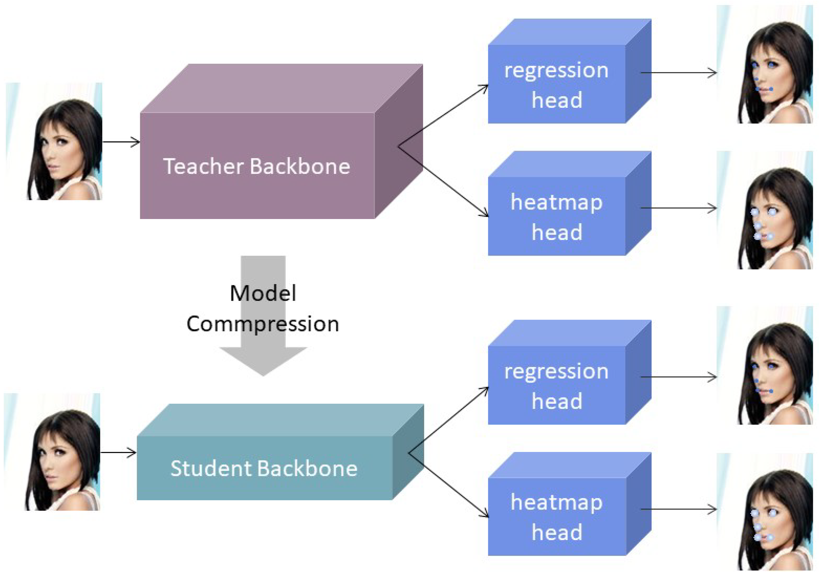
3.5. Model Compression

We introduce a model compression approach designed to distill a sizable Convolutional Neural Network (CNN) into a compressed yet performant counterpart, ensuring efficient execution while maintaining substantial accuracy levels. As depicted in Figure 2, our methodology follows a sequential paradigm, encompassing three crucial stages: an initial pre-training phase of the original network, a subsequent transfer of knowledge to an intermediary representation, and, finally, a model cutting step aimed at achieving the targeted compression level.

Pre-training of the network. Prior to the refinement and compression stages, the CNN undergoes an initial training phase on a comprehensive dataset, which serves as a foundation for subsequent learning on the targeted dataset. This pre-training strategy yields two pivotal benefits. Firstly, it functions as a potent regularization mechanism, bolstering the model’s ability to generalize beyond its training examples. By exposing the CNN to a vast corpus of data during pre-training, its parameters are optimized to capture the underlying data distribution more broadly, thereby mitigating the risk of overfitting to a limited subset of samples. Secondly, pre-training contributes to enhanced training stability and accelerated convergence. Convolutional networks, particularly those with intricate architectures and abundant parameters, can be susceptible to instabilities arising from random initialization of their parameters. By providing a supervised initialization through pre-training, the model is equipped with a robust starting point that fosters stable and efficient training processes.

We harness the extensive ImageNet dataset [27] as the cornerstone for pre-training. Prior to the targeted training phase on the specific image dataset, the CNN is initially pre-trained on ImageNet, a renowned benchmark in image recognition. Comprising 1.2 M images spanning 1000 prevalent categories, ImageNet offers a rich and diverse set of visual patterns to inform the CNN’s initial learning. This pre-training paradigm is universally applicable, benefiting both large-scale and more compact CNN architectures alike, by imparting a robust foundational knowledge base upon which further refinement can be built.

We introduce the notation Re for the pre-trained ResNet model and Mo for the MobileNet model, both of which constitute the CNN architectures pertinent to our methodology. These two models are further fine-tuned on the keypoint detection dataset with the LOSS function in a mini-batch manner. The LOSS function combines the output of the teacher model (Re) and the student model Mo with the joint modeling of regression and the heatmap. During this step, the two models are trained separately, with no interaction between them. With sufficient training, both models learn to detect face keypoints effectively.

In our approach, we designate the pre-trained ResNet and MobileNet models as Re and Mo, respectively, to distinguish their capacities. Subsequently, these models undergo additional training on the targeted image dataset, leveraging a mini-batch optimization strategy guided by a tailored LOSS function. This LOSS function integrates the predictions from both the teacher model (Re) and the student model Mo, incorporating joint modeling techniques for regression and heatmap generation. Notably, the training of Re and Mo proceeds independently. Through rigorous training, both models acquire the proficiency to accurately detect facial keypoints, demonstrating their effectiveness in learning the intricacies of the target task.

$$Lo\left(teacher\right)=LOSS$$

(4)

$$Lo\left(student\right)=LOSS$$

(5)

3.5.1. Knowledge Transfer

Following the above step, the teacher CNN (Re) is rendered static, and all the following optimization efforts are exclusively focused on the small CNN Mo. Given its inherently reduced parameter space, Mo inherently possesses a more constrained capacity for keypoint detection, translating to a comparatively diminished accuracy. To address this performance disparity, we introduce a mechanism aimed at transferring the keypoint detection to the smaller model. This approach endeavors to bridge the accuracy gap, empowering Mo to achieve a heightened level of precision that more closely aligns with that of Re.

Research has underscored the notion that the similarity of feature maps between a small and a large CNN, given identical input imagery, correlates strongly with the similarity of their predictions, thereby implying comparable capabilities. Leveraging this insight, we devise a transfer methodology aimed at aligning the feature maps of both networks at a designated layer. Specifically, the teacher model’s backbone produces a feature map ${\mathbf{M}}_r\in {\mathbb{R}}^{B\times C_{Lr}\times H_{Lr}\times W_{Lr}}$, whereas the student model’s backbone yields ${\mathbf{M}}_m\in {\mathbb{R}}^{B\times C_{Lm}\times H_{Lm}\times W_{Lm}}$. The disparity in these dimensions poses a challenge for direct knowledge transfer.

To overcome this obstacle, we employed average pooling to homogenize the dimensionality of both ${\mathbf{M}}_r$ and ${\mathbf{M}}_m$, yielding reduced representations ${\mathbf{M}}_r^{\prime }\in {\mathbb{R}}^{B\times C_{Lr}}$ and ${\mathbf{M}}_m^{\prime }\in {\mathbb{R}}^{B\times C_{Lm}}$, respectively. Furthermore, we utilized 1 × 1 convolutional layers to ensure that the vectors ${\mathbf{M}}_r\in {\mathbb{R}}^{B\times C_{La}}$ and ${\mathbf{A}}_m\in {\mathbb{R}}^{B\times C_{Lm}}$, derived from these reduced feature maps, share a common vector space dimensionality.

Finally, we adopted mean squared error (MSE) as the loss function, denoted as ${\mathrm{loss}}_3$, to quantify the discrepancy between corresponding elements in vectors ${\mathbf{a}}_r$ and ${\mathbf{a}}_m$ belonging to ${\mathbf{A}}_r$ and ${\mathbf{A}}_m$. This loss function computes the squared differences, facilitating the optimization process aimed at minimizing the divergence between the feature representations of the teacher and student models.

$${\mathit{loss}}_3=min{\displaystyle \frac{1}{B\times C_{Lm}}}\sum _{i=1}^B\sum _{j=1}^{C_{Lm}}{\left(a_{r_{ij}}-a_{m_{ij}}\right)}^2$$

(6)

3.5.2. Model Cutting

The overarching goal of this endeavor is to enhance the network’s efficiency by diminishing its parameter count, subsequently leading to a reduction in computational complexity. In the context of knowledge distillation, it is imperative that the parameter disparity between the teacher and student CNNs remains within a manageable threshold. This is due to the inherent learning constraints of the smaller CNN, where an excessively wide gap can hinder the effective transfer of knowledge. Consequently, the size of the student CNN cannot be overly diminutive, presenting a paradoxical challenge: maximizing efficiency while ensuring that the model does not sacrifice too much in terms of accuracy. To reconcile this dilemma, we introduce a model pruning or “cutting” strategy, tailored to strike an optimal balance between accuracy preservation and efficiency gains. This approach aims to meticulously identify and eliminate redundant or less impactful parameters, enabling the small CNN to achieve a highly efficient footprint while still retaining sufficient representational power to deliver acceptable levels of prediction accuracy.

We take the layer t in the network architecture as an example. The process of parameter reduction can be conceptualized as the elimination of insignificant filters within the tensor ${\mathbf{Z}}_t\in {\mathbb{R}}^{C_t\times C_{t-1}\times s\times s}$, essentially diminishing the count of filters in this layer. To quantify the significance of each filter, a logical approach involves assessing its impact on the subsequent feature maps, where less influential filters exhibit reduced effects. Specifically, upon hypothetically removing a filter, the dimensionality of ${\mathbf{Z}}_t$ would adjust to ${\mathbb{R}}^{C_{t-1}\times C_{t-1}\times s\times s}$, with corresponding alterations in the feature maps ${\mathbf{M}}_t\in {\mathbb{R}}^{C_{t-1}\times H\times W}$ and the subsequent convolutional kernel ${\mathbf{Z}}_{t+1}\in {\mathbb{R}}^{C_{t+1}\times C_{t-1}\times s\times s}$, leading to an altered feature map ${\mathbf{M}}_{t+1}\in {\mathbb{R}}^{C_{t+1}\times H\times W}$.

To objectively evaluate the importance of each filter, we leverage a subset of images and employ the adjacent, unmodified feature map ${\mathbf{M}}_{t+1}$ as a reference. By sequentially removing each filter and computing the resultant reconstruction error for the reference map, we can infer the significance of each filter. This methodology enables us to identify and prune those filters that contribute minimally to the overall representation, thereby refining the model’s efficiency without unduly compromising its accuracy.

$${\mathit{Score}}^{Ci}={\displaystyle \frac{{\sum }_{l=1}^L{∥{\mathbf{M}}_{t+1}^{Ci}\left(s_l\right)-{\mathbf{M}}_{t+1}\left(s_l\right)∥}_2^2}{L}}$$

(7)

Within the sampled subset $\left\{s_l\right|l=1,\dots ,L,L\ll N\}$, where L is significantly smaller than the number of training images N, ${\mathbf{M}}_{t+1}^i\left(s_l\right)$ denotes the transformed representation subsequent to the removal of the i-th filter from the set of filters at layer t. The significance metric is derived by assessing the impact of eliminating the i-th filter from ${\mathbf{Z}}_t$. By arranging these significance metrics in descending order, we can systematically prune filters with lower scores, guided by a predetermined pruning ratio $\alpha$. Specifically, we discard $⌈{\mathbf{Z}}_t\times \alpha ⌉$ filters while retaining $⌈{\mathbf{Z}}_t\times (1-\alpha )⌉$ filters, thereby generating a refined set of filters for the t-th layer, denoted as ${\mathbf{Z}}_t\in {\mathbb{R}}^{⌈C_t\times (1-\alpha )⌉\times C_{t-1}\times s\times s}$. This process ensures that the new filter configuration at each layer is optimized for both efficiency and performance considerations.

While the contribution of less significant filters may be modest, they nevertheless encode image representations that could potentially contribute positively to the model’s performance. Consequently, their straightforward elimination can result in a decrement in the network’s detection capabilities. To counteract this potential loss, a widely adopted strategy involves subjecting the pruned network to a retraining process, which enables the remaining filters to adapt and learn the requisite image representations more comprehensively. In this regard, we employed the entire dataset to retrain the downsized CNN, adhering to the same training paradigm outlined in Equation (8), thereby fostering the network’s ability to maintain or even enhance its detection accuracy.

$${\mathit{loss}}_t=LOSS+{\mathit{loss}}_3$$

(8)

Ultimately, we used an layer-wise pruning methodology where layers are successively reduced, commencing from layer T and progressing downwards to layer 1 within the transferred student model $St{u}^K$. For each intermediate layer t, the pruning process closely mirrors the above procedure. Notably, the pruning ratio $\alpha$ serves as a tunable parameter, allowing us to tailor the model’s efficiency to meet diverse requirements. However, it is imperative to strike a delicate balance between optimizing efficiency and preserving accuracy, as adjustments to $\alpha$ can have consequential impacts on both aspects. Following the completion of this top–down iterative pruning process across all layers, the resulting $S_{tu}$ represents the final compressed student model, optimized for both efficiency and performance.

4. Experimental Results

In this section, we evaluate the proposed methods. We first introduce the experimental setup in detail and then present the main results of regression combined with a heatmap network and pruning combined with distillation supervision.

4.1. Detailed Setup

Database: for this experiment, we used three datasets: 300W [28], AFLW [29], and CelebA. The 300W and AFLW datasets were utilized for training and testing, while the CelebA dataset was employed for ablation studies.

300W: this dataset includes annotations for five face datasets—LFPW, AFW, HELEN, XM2VTS, and IBUG—with 68 landmarks each. It includes [30,31,32] 3148 images for training and 689 images for testing. The test images are divided into a common subset and a challenge subset: the common subset consists of 554 images from LFPW and HELEN, and the challenge subset comprises 135 images from IBUG.

AFLW: this dataset contains 24,386 wild faces, sourced from Flickr, featuring extreme poses, expressions, and occlusions. The facial head poses range from 0° to 120° (yaw angle) and 90° (pitch and roll angles). AFLW provides up to 21 landmarks per face. We used 20,000 images for training and 4386 images for testing.

CelebA: for ablation and hyperparameter experiments, we used the CelebA dataset, which contains 10,177 identities and 202,599 face images. Each image is annotated with features, including face bounding boxes, five face keypoint coordinates, and 40 attribute labels. We split the dataset into training and validation sets, using 80% for training and 20% for validation.

Backbone network: for the teacher model, we used the popular ResNet-50 network, which is sufficiently deep to handle our tasks. The core idea is that, by introducing residual blocks, the input can bypass one or more convolutional layers and directly add to the output. This approach solves the problems of gradient vanishing in deep network training by using identity mapping. For the student model, we used the MobileNet network. Its core feature is depthwise convolution, which splits standard convolution into two independent operations: depthwise convolution and $1\times 1$ convolution. This greatly reduces parameters and computation, thereby improving training efficiency.

Data processing: the face images in the original CelebA dataset were cropped to allow the model to focus more on learning face features and keypoints. To increase the generalization of training, we performed data augmentation on the CelebA dataset by randomly flipping some images horizontally to simulate different shooting angles and cropping face images in different regions to increase data diversity and model robustness.

Training strategy: we set the epoch, batch size, and learning rate as follows. For the batch size, whether it is the combined training of regression and heatmap or the combined optimization of distillation and pruning, we fixed the value at 32. For the learning rate, the pre-trained model based on ImageNet was adjusted from 0.01 to 0.0001 every 20 epochs, for a total of 60 epochs.

Evaluation criteria: for the 300W, ALFW, and CelebA datasets, the evaluation metrics differed slightly. In the case of the 300W dataset, results were reported using two different normalizing factors. One used the eye-center distance as the inter-pupil normalizing factor, while the other was based on the inter-ocular distance, measured as the distance between the outer corners of the eyes. For the ALFW dataset, due to the presence of various facial profiles, the error was normalized according to the ground-truth bounding box size across all visible landmarks. For the CelebA dataset, the mean square error (MSE) was used as the evaluation metric. We compared the mean squared error (MSE) results for regression combined with the heatmap under different weight ratios, as well as the MSE results for pruning combined with distillation under various weight ratios. Additionally, we compared the MSE results across different pruning rates.

4.2. Main Results

This section begins with a detailed comparative analysis of the proposed method against existing facial keypoint detection methods. We then introduce the evaluation method that combines the heatmap and regression, as well as the evaluation method that combines distillation and pruning. Additionally, we discuss the impact of different loss weights on regression combined with the heatmap, distillation combined with pruning, and the effects of varying pruning rates.

4.2.1. Comparison with Existing Methods

We first compared the mobile–distill–prune model and ResNet-50 with state-of-the-art face landmark detection methods on a 300W dataset using a regression combined with a heatmap approach. The results are shown in

Table 1. Normalized mean error comparison of the 300W dataset’s common subset, challenging subset, and full set. The bold entries represent the model proposed in this paper.

Method	Common	Challenging	Fullset
Inter-pupil Normalization (IPN)
RCPR [33]	6.18	17.26	8.35
CFAN [34]	5.50	16.78	7.69
ESR [35]	5.28	17.00	7.58
SDM [36]	5.57	15.40	7.50
LBF [37]	4.95	11.98	6.32
CFSS [38]	4.73	9.98	5.76
3DDFA [39]	6.15	10.59	7.01
TCDCN [40]	4.80	8.60	5.54
MDM [41]	4.83	10.14	5.88
SeqMT [42]	4.84	9.93	5.74
RAR [43]	4.12	8.35	4.94
DVLN [44]	3.94	7.62	4.66
CPM [45]	3.39	8.14	4.36
DCFE [46]	3.83	7.54	4.55
TSR [47]	4.36	7.56	4.99
LAB [31]	3.42	6.98	4.12
PFLD 0.25X [1]	3.38	6.83	4.02
PFLD 1X [1]	3.32	6.56	3.95
Mobile–distill–prune-0.25X (vs. PFLD 0.25X [1])	3.36 (+0.59%)	6.78 (+0.73%)	3.98 (+0.99%)
Mobile–distill–prune-1X (vs. PFLD 1X [1])	3.24 (+2.4%)	6.54 (+0.3%)	3.89 (+1.5%)
ResNet-50	3.20	6.48	3.87
Inter-ocular Normalization (ION)
PIFA-CNN [48]	5.43	9.88	6.30
RDR [49]	5.03	8.95	5.80
PCD-CNN [32]	3.67	7.62	4.44
SAN [30]	3.34	6.60	3.98
PFLD 0.25X [1]	3.03	5.15	3.45
PFLD 1X [1]	3.01	5.08	3.40
Mobile–distill–prune-0.25X (vs. PFLD 0.25X [1])	3.02 (+0.3%)	5.14 (+0.19%)	3.44 (+0.28%)
Mobile–distill–prune-1X (vs. PFLD 1X [1])	2.98 (+0.99%)	5.04 (+0.78%)	3.38 (+0.58%)
ResNet-50	2.96	4.96	3.34

. To comprehensively evaluate model performance, we report two versions of the mobile–distill–prune model: mobile–distill–prune-0.25X and mobile–distill–prune-1X. Mobile–distill–prune-0.25X compresses the model by setting the pruning rate to 75%, while mobile–distill–prune-1X is the full model without pruning. Both models were trained using only the 300W training data. Additionally, we include the performance of ResNet-50 for comparison.

Although the performance of mobile–distill–prune-0.25X is slightly lower than that of mobile–distill–prune-1X, it still outperforms other competitors in many aspects, demonstrating excellent detection capabilities. This comparison shows that mobile–distill–prune-0.25X finds a good balance between model compression and detection accuracy. Despite significant reduction in model size through pruning, the detection accuracy does not drop substantially, making it an ideal compromise for practical applications.

ResNet-50 consistently shows the best overall performance among all the models tested, especially in handling challenging facial data. This indicates that ResNet-50 has strong feature extraction capabilities and robustness. However, this also highlights areas for improvement in the mobile–distill–prune model. By further optimizing the balance between pruning and distillation, the performance of the mobile–distill–prune model may be enhanced, bringing it closer to ResNet-50’s level of detection accuracy.

We further evaluated the performance differences of various methods on the AFLW dataset. The AFLW value results obtained by these methods are reported in

Table 2. Normalized mean error comparison on the AFLW–full dataset. The bold entries represent the model proposed in this paper.

Method	RCPR [33]	CDM [50]	SDM [36]	ERT [51]	LBF [37]	CFSS [38]	CCL [52]	Binary-CNN [53]	PCD-CNN [32]
AFLW	5.43	3.73	4.05	4.35	4.25	3.92	2.72	2.85	2.40
Method	TSR [47]	CPM [45]	SAN [30]	PFLD 0.25X [1]	PFLD 1X [1]	mobile–distill–prune-0.25X	mobile–distill–prune-1X	ResNet-50
AFLW	2.17	2.33	1.91	2.07	1.88	2.06	1.86	1.84

. As can be seen from the table, methods including TSR, CPM, SAN, PFLD, and our mobile–distill–prune series, as well as ResNet-50, significantly outperform other competing methods. Among these outstanding methods, our ResNet-50 achieved the best accuracy (NME 1.84), followed by our mobile–distill–prune-1X (NME 1.86). PFLD 1X ranked third with an NME value of 1.88.

In summary, our experiments demonstrate the advantages and disadvantages of different models on the 300W dataset through the combination of regression with a heatmap and the comprehensive application of distillation and pruning techniques. Although mobile–distill–prune-0.25X is slightly inferior to mobile–distill–prune-1X in performance, it achieves a satisfactory balance between model size and detection accuracy. ResNet-50 leads in overall performance, particularly when processing complex facial data. The experimental results verify the effectiveness of our proposed method and provide new insights and methodologies in the field of facial keypoint detection. By combining advanced deep learning techniques such as model distillation, pruning, and efficient neural network architecture design, we can significantly optimize the computational efficiency and applicability of the model while maintaining high accuracy. This provides an important reference for the future deployment of efficient and accurate facial feature point detection models in practical applications.

4.2.2. Regression Combined with Heatmap Results

To demonstrate the effectiveness of heatmaps in face keypoint detection, we conducted a series of comparative experiments to evaluate the detection performance when using only the regression model and when adding heatmaps. Figure 3 presents the experimental results of facial keypoint detection across various environments.

In the base regression model, we directly predicted the coordinates of the keypoints and obtained a mean square error (MSE LOSS) of 0.0556. Next, we added heatmaps as an intermediate representation for keypoint detection. By generating a heatmap on the label image, we further captured and utilized the heat value at the location of each keypoint in the image. The experimental results are presented in

Table 3. Comparison of the performance between regression alone and regression combined with heatmap.

Backbone	Algorithm	MSE	t-Test/p-Value	Levene-Test/ p-Value
MobileNet	regression	0.0556	T: 0.52, 0.97, 0.44	L: 0.73, 1.23, 0.06
			P: 0.59, 0.32, 0.65	P: 0.39, 0.26, 0.80
MobileNet	regression + heatmap	0.0462	T: 0.64, 0.93, 0.29	L: 0.03, 1.87, 1.28
			P: 0.52, 0.34, 0.76	P: 0.84, 0.34, 0.25

, which show that the MSE LOSS significantly decreased to 0.0462 after adding the heatmap, representing an improvement of 16.90%. To evaluate the generalization ability of our regression algorithm and the regression combined with the heatmap algorithm, we utilized a three-fold cross-validation method, involving pairwise combinations of three different test sets, thus yielding three validation values and corresponding p-values for each set of experiments. Performance metrics were collected for each fold to ensure robust evaluation. We applied the t-values to examine the mean differences in performance metrics across the folds. Additionally, the Levene test was employed to check for homogeneity of variances. Large p-values from both the t-values and Levene test were observed, indicating that the mean performance differences were not statistically significant, and the variances were homogeneous.

The reason for this improvement is that heatmaps provide more detailed local information, making the model more robust and accurate when processing keypoints in specific areas of the image. Heatmaps are particularly effective in capturing the location of keypoints in challenging scenarios involving large angles, occlusion, or complex lighting conditions, thereby improving the overall performance of the model.

4.2.3. Distillation Combined with Pruning Results

To show how effective it is to combine distillation with pruning in face keypoint detection, we carried out multiple experiments and compared the detection results of various model combinations. These combinations included regression + heatmap, regression + heatmap + distillation, and regression + heatmap + distillation + pruning.

As shown in

Table 4. Performance comparison of distillation combined with pruning based on regression and heatmap.

Backbone	Algorithm	MSE	t-Test/p-Value	Levene-Test/p-Value
ResNet-50	regression + heatmap	0.0457	T: 0.13, 0.48, 0.35	L: 1.21, 1.55, 0.02
			P: 0.89, 0.62, 0.72	P: 0.26, 0.21, 0.88
MobileNet	regression + heatmap	0.0462	T: 0.64, 0.93, 0.29	L: 0.03, 1.87, 1.28
			P: 0.52, 0.34, 0.76	P: 0.84, 0.34, 0.25
MobileNet	regression + heatmap + distillation	0.0434	T: 0.49, 0.54, 0.05	L: 0.15, 0.02, 0.29
			P: 0.61, 0.58, 0.95	P: 0.69, 0.88, 0.58
MobileNet	regression + heatmap + distillation + pruning (50%)	0.0445	T: 0.18, 0.63, 0.45	L: 0.98, 0.42, 0.09
			P: 0.85, 0.52, 0.65	P: 0.34, 0.51, 0.76

, a teacher model was developed and evaluated using the regression + heatmap approach, achieving an MSE LOSS of 0.0457. In parallel, a student model was created and assessed with the same regression + heatmap approach, resulting in an MSE LOSS of 0.0462.

To enhance the student model’s accuracy, we incorporated a distillation step into the regression + heatmap method, transferring knowledge from the teacher model to the student model. This process lowered the MSE LOSS of the student model to 0.0434. The process of knowledge distillation enabled the lightweight student model to better learn the deep features from the teacher model, thereby improving its detection accuracy. Building on this, we further incorporated a pruning step, pruning 50% of the student model to remove redundant parameters. The experimental results showed that the MSE LOSS of the pruned student model was 0.0445. Although there is a slight increase, compared to the unpruned student model, the pruned model significantly reduced computation and model size while maintaining high precision, thus improving the model efficiency. The improvement is attributed to the combination of distillation and pruning, which allows the network to be trained and optimized with minimal accuracy loss. Distillation helps the lightweight models learn more powerful representations, while pruning optimizes the model structure, making it more efficient and lightweight.

To assess the generalization capability of various algorithms, including regression + heatmap on ResNet-50, regression + heatmap on MobileNet, regression + heatmap + distillation on MobileNet, and regression + heatmap + distillation + pruning (50%) on MobileNet, we conducted a three-fold cross-validation. This method involved pairwise combinations of three different test sets, thus yielding three validation values and corresponding p-values for each set of experiments. Performance metrics were collected for each fold to ensure a thorough evaluation. We applied the t-values to examine the mean differences in performance metrics across the folds and employed the Levene test to check for homogeneity of variances. The large p-values from both the t-test and Levene test indicated that the mean performance differences were not statistically significant and the variances were homogeneous.

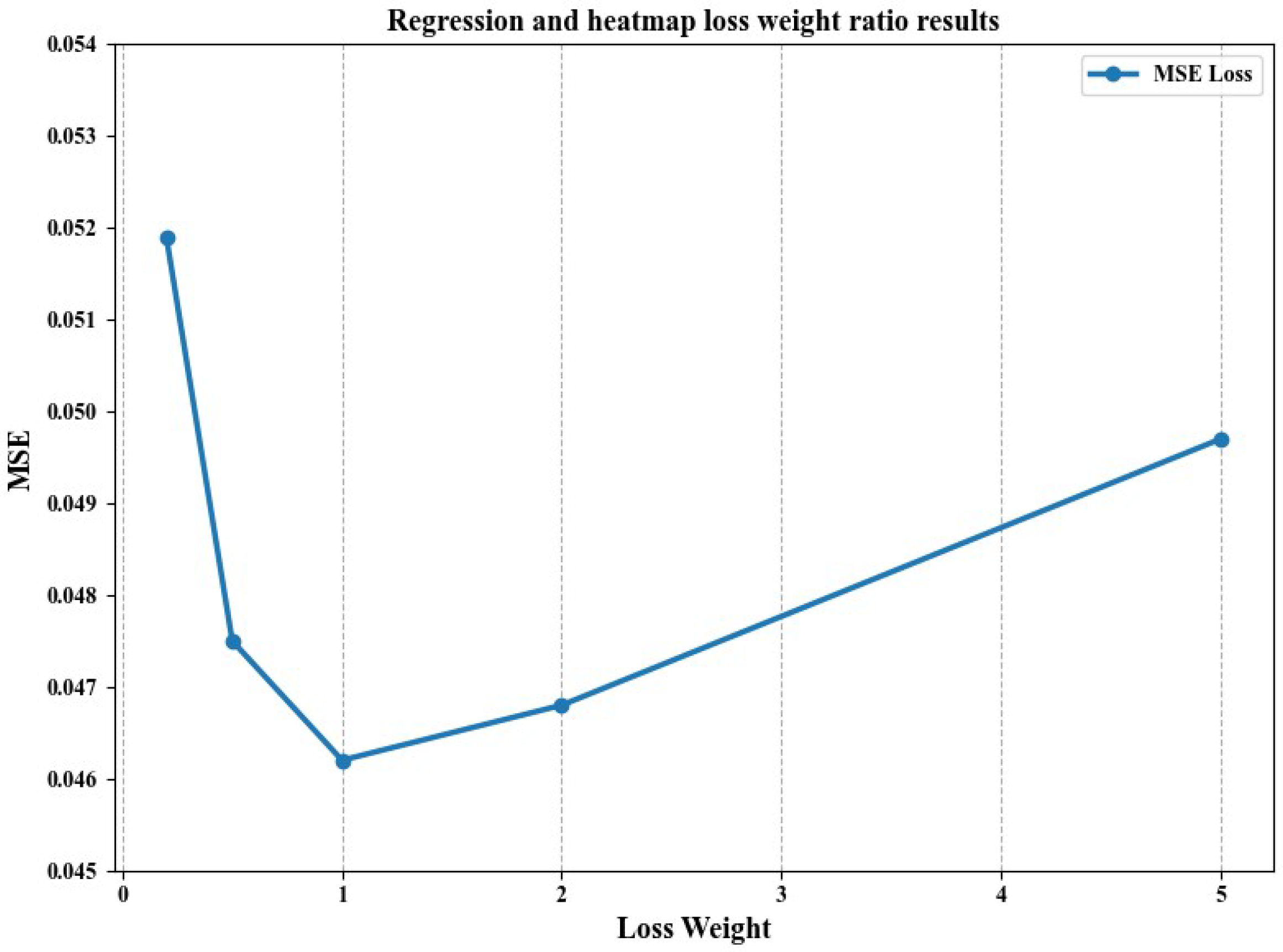
4.2.4. Regression and Heatmap Loss Weight Ratio Results

To evaluate the influence of different regression and heatmap loss weight combinations on model performance, we adjusted the weight ratio of these two losses to find the optimal balance between regression accuracy and heatmap quality. The weight ratio of regression to heatmap is denoted as ${\lambda }_{rh}$.

$${\lambda }_{rh}\in \left\{0.2,0.5,1,2,5\right\}$$

(9)

The results of the comparative experiments are shown in Figure 4, where we found that, when the weight ratio is 1, the minimum MSE value is 0.0462. When the weight ratio deviates from the optimal range, the mean squared error (MSE) value increases, leading to worse performance. This is because, when the weight ratio is close to 1, the model can effectively balance between predicting global keypoint coordinates and expressing local heatmap details. This equilibrium enables accurate keypoint prediction and detailed feature refinement, while also preventing significant differences during gradient updates, thus avoiding issues like gradient explosion or vanishing. If the weight ratio exceeds 1, the model prioritizes global coordinate prediction but lacks in capturing local details, which hampers its ability to refine keypoint positions, especially under conditions of severe occlusion. On the other hand, if the weight ratio is below 1, the model overly focuses on local heatmap features at the expense of global keypoint accuracy. This results in the poor capture of global structures and overfitting to local details.

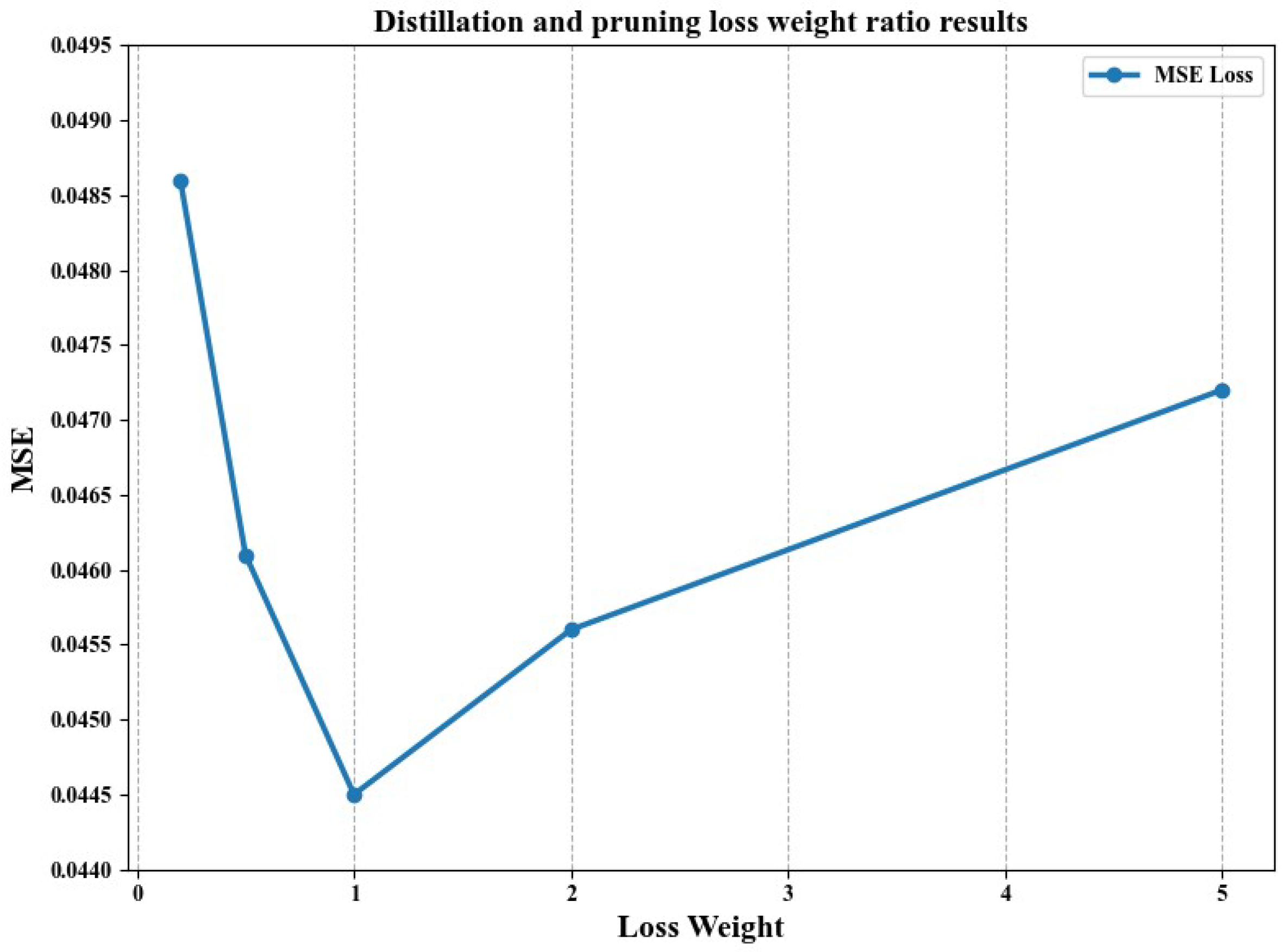
4.2.5. The Result of Distillation and Pruning Loss Weight Ratio

Regarding experiments investigating the effect of loss weights on distillation combined with pruning, Figure 5 presents the results. We studied the impacts of different distillation and pruning loss weights on model performance. By adjusting the weight ratio ${\lambda }_{dp}$ of these two losses, we aimed to minimize model size and computational cost while maintaining accuracy.

$${\lambda }_{dp}\in \left\{0.2,0.5,1,2,5\right\}$$

(10)

The experimental results show that, under the conditions of a weight ratio of 1 and a regression pruning rate of 50%, the best performance is achieved with an MSE of 0.0445 when the distillation and pruning loss weights are equal. This balance allows the model to achieve compression while maintaining accuracy. When the distillation weight is too small, the MSE is 0.0486, indicating that the student model cannot effectively learn from the teacher model, resulting in deteriorated performance. Conversely, when the distillation weight is too large, the MSE is 0.0472, as the overemphasis on distillation loss neglects the role of pruning, failing to effectively reduce the model size and computational cost.

4.2.6. Experimental Results of Different Pruning Rates

Pruning rate refers to the proportion of parameters that are removed from the model. Pruning can reduce the computational load and the number of parameters, thereby improving the operational efficiency of the model. To further study the effect of pruning techniques on model performance, we set different pruning rates r for comparative experiments. By comparing the model’s performance on the verification set under various pruning rates, we evaluated the impact on model accuracy and computational efficiency to identify the optimal pruning rate.

$$r\in \left\{10\%,30\%,50\%,70\%,90\%\right\}$$

(11)

With the pruning rate r = 10%, the MSE of the model on the verification set was 0.0438. As the pruning rate increased, computational efficiency improved, but model accuracy decreased. When the pruning rate r = 90%, the MSE increased to 0.0478, resulting in a precision loss of 9.13% compared to the model without pruning. The experimental results presented in Figure 6 indicate that a low pruning rate (e.g., 10%) has minimal impact on model accuracy, but the improvement in computational efficiency is limited. Conversely, a high pruning rate (e.g., 90%) significantly reduces the computational load but also leads to a substantial loss in accuracy.

4.2.7. Performance Analysis of Model Size, Computational Speed, and Running on Mobile Devices

Model size: as shown in

Table 5. Comparison of model size and processing speed with existing methods. The bold entries represent the model proposed in this paper.

Model	SDM [36]	SAN [30]	LAB [31]	PFLD 0.25X [1]	PFLD 1X [1]	mobile– distill– prune-0.25x	mobile– distill– prune-1x
Size (Mb)	10.1	270.5 + 528	50.7	2.1	12.5	2.5	7.8
Speed	16 ms (C)	343 ms (G)	2.6 s (C) 60 ms (G*)	1.2 ms (C) 1.2 ms (G) 7 ms (A)	6.1 ms (C) 3.5 ms (G) 26.4 ms (A)	2 ms (C) 1.9 ms (G) 12 ms (A)	4.5 ms (C) 3.6 ms (G) 18.7 ms (A)

, our model, mobile–distill–prune-0.25x, is significantly smaller at 2.5 Mb, saving over 5 Mb compared to the mobile–distill–prune-1x. This reduction makes mobile–distill–prune-0.25x much more compact than most models, such as SDM (10.1 Mb), LAB (50.7 Mb), and SAN, which is around 800 Mb with its two VGG-based subnets measuring 270.5 Mb and 528 Mb, respectively.

Processing speed: we measure the efficiency of each algorithm using an i7-6700K CPU(Intel Corporation, Santa Clara, CA, USA) (denoted as C) and an Nvidia GTX 1080Ti GPU, Nvidia, Santa Clara, CA, USA (denoted as G), unless stated otherwise. Since only the CPU version of SDM [36] and the GPU version of SAN [30] are publicly available, their times are reported accordingly. For LAB [31], only the CPU version is available for download, but the authors mention in their paper [31] that their algorithm runs in approximately 60 ms on a TITAN X GPU (denoted as G*). Our results show that mobile–distill–prune-0.25x and mobile–distill–prune-1x outperform most algorithms in terms of speed on both CPU and GPU. Notably, LAB’s CPU time is reported in seconds rather than milliseconds. Furthermore, mobile–distill–prune-1x required 2.25 times the CPU time and 1.89 times the GPU time compared to mobile–distill–prune-0.25x. Despite this, PFLD 1X remained much faster than the other models. Additionally, for PFLD 0.25X and PFLD 1X, we conducted tests on a Qualcomm ARM 845 processor (denoted as A). Here, mobile–distill–prune-0.25x processed a face in 12 ms (over 83 fps), while mobile–distill–prune-1x processed a face in 18.7 ms (over 53 fps).

Mobile terminal evaluation:

Table 6. Comparing model performance on three different mobile devices. The bold entries represent the model proposed in this paper.

Mobile	HUAWEI Mate9 Pro	Xiaomi MI 9	HUAWEI P30 Pro
CPU	Kirin960	Snapdragon855	Kirin980
Frequency	$4\times 2.4$ GHz + $4\times 1.8$ GHz	$1\times 2.84$ GHz + $3\times 2.42$ GHz + $4\times 1.78$ GHz	$2\times 2.6$ GHz + $2\times 1.92$ GHz + $4\times 1.8$ GHz
RAM	4 GB	8 GB	8 GB
ResNet50	87 ms	63 ms	49 ms
Mobile–distill–prune-1x	31 ms	18 ms	14 ms
Mobile–distill–prune-0.25x	19 ms	13 ms	11 ms

shows the performance comparison of different models on three mobile devices (HUAWEI Mate9 Pro, HUAWEI Technologies Co., Ltd., Shenzhen, China; Xiaomi 9, Xiaomi Corporation, Beijing, China; and HUAWEI P30 Pro, HUAWEI Technologies Co., Ltd., Shenzhen, China). The comparison indicators include CPU specifications, RAM, and processing speed (in milliseconds).

Among all devices, the mobile–distill–prune-1x and mobile–distill–prune-0.25x models are significantly faster, with the mobile–distill–prune-0.25x model being the fastest, reaching a processing speed of 11ms on the HUAWEI P30 Pro. While maintaining high accuracy, it greatly reduces the computational complexity and storage requirements of the model, allowing for inference in a very short time. This has important practical significance for real-time application scenarios such as facial recognition, augmented reality, and intelligent monitoring.

5. Conclusions

This paper addressed the robustness of face keypoint detection, focusing on effective and efficient detection in challenging environments such as occlusion and inversion. Our key contributions are as follows. Effectiveness enhancement: we proposed a novel approach that combines regression and heatmap training, inspired by the concept of human keypoints. This method significantly improves the accuracy and reliability of face keypoint detection, even under extreme conditions. Efficiency improvement: to reduce the model’s computational load, we introduced a compression method that integrates distillation and pruning. This approach effectively minimizes the model size while maintaining high performance, making it suitable for deployment on resource-constrained devices. Integrated technique: we successfully combined regression, heatmap, pruning, and distillation techniques into a cohesive framework. Our comprehensive experiments demonstrated the robustness and superiority of our method compared to existing approaches, especially in terms of speed and accuracy. Experimental validation: through detailed experiments, we compared our method with existing deep learning approaches and used significant statistical analyses to demonstrate the robustness and generalization ability of our model’s performance. In ablation experiments and hyperparameter studies, we examined the impact of combining regression with heatmap training and pruning with distillation on the algorithm’s accuracy. Finally, we conducted a comparative study on model size, computational speed, and mobile device detection. The research data validated the efficiency, effectiveness, and lightweight nature of the method proposed in this paper.

Our findings have important practical implications for real-time applications such as facial recognition, augmented reality, and intelligent monitoring. The ability to detect face keypoints accurately and efficiently, even in extreme conditions, enhances the usability and reliability of these applications. Our model’s reduced computational complexity and storage requirements make it ideal for deployment on mobile devices and other platforms with limited resources. While our approach demonstrates robustness in occlusion and inversion scenarios, there may still be edge cases where performance could be improved. Future research should focus on enhancing the model’s ability to handle more complex and varied occlusions. Additionally, further exploration into the synergistic effects of combining different techniques, such as advanced pruning methods and more sophisticated distillation strategies, could result in even more efficient models.

References

1. Guo, X.; Li, S.; Yu, J.; Zhang, J.; Ma, J.; Ma, L.; Liu, W.; Ling, H. PFLD: A practical facial landmark detector. arXiv 2019, arXiv:1902.10859. [Google Scholar]
2. Wang, X.; Bo, L.; Fuxin, L. Adaptive wing loss for robust face alignment via heatmap regression. In Proceedings of the IEEE/CVF International Conference on Computer Vision, Seoul, Republic of Korea, 27 October–2 November 2019; pp. 6971–6981. [Google Scholar]
3. Wang, J.; Sun, K.; Cheng, T.; Jiang, B.; Deng, C.; Zhao, Y.; Liu, D.; Mu, Y.; Tan, M.; Wang, X.; et al. Deep high-resolution representation learning for visual recognition. IEEE Trans. Pattern Anal. Mach. Intell. 2020, 43, 3349–3364. [Google Scholar] [CrossRef] [PubMed]
4. Xu, Y.; Yan, W.; Yang, G.; Luo, J.; Li, T.; He, J. CenterFace: Joint face detection and alignment using face as point. Sci. Program. 2020, 2020, 7845384. [Google Scholar] [CrossRef]
5. Browatzki, B.; Wallraven, C. 3FabRec: Fast few-shot face alignment by reconstruction. In Proceedings of the IEEE/CVF Conference on Computer Vision and Pattern Recognition, Seattle, WA, USA, 13–19 June 2020; pp. 6110–6120. [Google Scholar]
6. Liu, Z.; Lin, W.; Li, X.; Rao, Q.; Jiang, T.; Han, M.; Fan, H.; Sun, J.; Liu, S. ADNet: Attention-guided deformable convolutional network for high dynamic range imaging. In Proceedings of the IEEE/CVF Conference on Computer Vision and Pattern Recognition, Nashville, TN, USA, 20–25 June 2021; pp. 463–470. [Google Scholar]
7. Li, Y.; Yang, S.; Liu, P.; Zhang, S.; Wang, Y.; Wang, Z.; Yang, W.; Xia, S.T. Simcc: A simple coordinate classification perspective for human pose estimation. In Proceedings of the European Conference on Computer Vision, Tel Aviv, Israel, 23–27 October 2022; pp. 89–106. [Google Scholar]
8. Bai, Y.; Wang, A.; Kortylewski, A.; Yuille, A. Coke: Contrastive learning for robust keypoint detection. In Proceedings of the IEEE/CVF Winter Conference on Applications of Computer Vision, Waikoloa, HI, USA, 2–7 January 2023; pp. 65–74. [Google Scholar]
9. Wan, J.; Liu, J.; Zhou, J.; Lai, Z.; Shen, L.; Sun, H.; Xiong, P.; Min, W. Precise facial landmark detection by reference heatmap transformer. IEEE Trans. Image Process. 2023, 32, 1966–1977. [Google Scholar] [CrossRef] [PubMed]
10. Yu, Z.; Huang, H.; Chen, W.; Su, Y.; Liu, Y.; Wang, X. Yolo-facev2: A scale and occlusion aware face detector. Pattern Recognit. 2024, 155, 110714. [Google Scholar] [CrossRef]
11. Rangayya; Virupakshappa; Patil, N. Improved face recognition method using SVM-MRF with KTBD based KCM segmentation approach. Int. J. Syst. Assur. Eng. Manag. 2024, 15, 1–12. [Google Scholar] [CrossRef]
12. Khan, S.S.; Sengupta, D.; Ghosh, A.; Chaudhuri, A. MTCNN++: A CNN-based face detection algorithm inspired by MTCNN. Vis. Comput. 2024, 40, 899–917. [Google Scholar] [CrossRef]
13. Blalock, D.; Gonzalez Ortiz, J.J.; Frankle, J.; Guttag, J. What is the state of neural network pruning? Proc. Mach. Learn. Syst. 2020, 2, 129–146. [Google Scholar]
14. Vadera, S.; Ameen, S. Methods for pruning deep neural networks. IEEE Access 2022, 10, 63280–63300. [Google Scholar] [CrossRef]
15. Fang, G.; Ma, X.; Song, M.; Mi, M.B.; Wang, X. Depgraph: Towards any structural pruning. In Proceedings of the IEEE/CVF Conference on Computer Vision and Pattern Recognition, Vancouver, BC, Canada, 17–24 June 2023; pp. 16091–16101. [Google Scholar]
16. Sun, M.; Liu, Z.; Bair, A.; Kolter, J.Z. A simple and effective pruning approach for large language models. arXiv 2023, arXiv:2306.11695. [Google Scholar]
17. Ji, M.; Heo, B.; Park, S. Show, attend and distill: Knowledge distillation via attention-based feature matching. In Proceedings of the AAAI Conference on Artificial Intelligence, Online, 2–9 February 2021; Volume 35, pp. 7945–7952. [Google Scholar]
18. Yao, Y.; Huang, S.; Wang, W.; Dong, L.; Wei, F. Adapt-and-distill: Developing small, fast and effective pretrained language models for domains. arXiv 2021, arXiv:2106.13474. [Google Scholar]
19. Beyer, L.; Zhai, X.; Royer, A.; Markeeva, L.; Anil, R.; Kolesnikov, A. Knowledge distillation: A good teacher is patient and consistent. In Proceedings of the IEEE/CVF Conference on Computer Vision and Pattern Recognition, New Orleans, LA, USA, 18–24 June 2022; pp. 10925–10934. [Google Scholar]
20. Park, J.; No, A. Prune your model before distill it. In Proceedings of the European Conference on Computer Vision, Glasgow, UK, 23–27 October 2022; pp. 120–136. [Google Scholar]
21. Waheed, A.; Kadaoui, K.; Abdul-Mageed, M. To Distill or Not to Distill? On the Robustness of Robust Knowledge Distillation. arXiv 2024, arXiv:2406.04512. [Google Scholar]
22. He, K.; Zhang, X.; Ren, S.; Sun, J. Deep residual learning for image recognition. In Proceedings of the IEEE Conference on Computer Vision and Pattern Recognition, Las Vegas, NV, USA, 27–30 June 2016; pp. 770–778. [Google Scholar]
23. Xie, S.; Girshick, R.; Dollár, P.; Tu, Z.; He, K. Aggregated residual transformations for deep neural networks. In Proceedings of the IEEE Conference on Computer Vision and Pattern Recognition, Honolulu, HI, USA, 21–26 July 2017; pp. 1492–1500. [Google Scholar]
24. Howard, A.G.; Zhu, M.; Chen, B.; Kalenichenko, D.; Wang, W.; Weyand, T.; Andreetto, M.; Adam, H. Mobilenets: Efficient convolutional neural networks for mobile vision applications. arXiv 2017, arXiv:1704.04861. [Google Scholar]
25. Sandler, M.; Howard, A.; Zhu, M.; Zhmoginov, A.; Chen, L.C. Mobilenetv2: Inverted residuals and linear bottlenecks. In Proceedings of the IEEE Conference on Computer Vision and Pattern Recognition, Salt Lake City, UT, USA, 18–23 June 2018; pp. 4510–4520. [Google Scholar]
26. Howard, A.; Sandler, M.; Chu, G.; Chen, L.C.; Chen, B.; Tan, M.; Wang, W.; Zhu, Y.; Pang, R.; Vasudevan, V.; et al. Searching for mobilenetv3. In Proceedings of the IEEE/CVF International Conference on Computer Vision, Seoul, Republic of Korea, 27 October–2 November 2019; pp. 1314–1324. [Google Scholar]
27. Deng, J.; Dong, W.; Socher, R.; Li, L.J.; Li, K.; Fei-Fei, L. Imagenet: A large-scale hierarchical image database. In Proceedings of the 2009 IEEE Conference on Computer Vision and Pattern Recognition, Miami, FL, USA, 20–25 June 2009; pp. 248–255. [Google Scholar]
28. Sagonas, C.; Tzimiropoulos, G.; Zafeiriou, S.; Pantic, M. 300 faces in-the-wild challenge: The first facial landmark localization challenge. In Proceedings of the IEEE International Conference on Computer Vision Workshops, Sydney, NSW, Australia, 1–8 December 2013; pp. 397–403. [Google Scholar]
29. Koestinger, M.; Wohlhart, P.; Roth, P.M.; Bischof, H. Annotated facial landmarks in the wild: A large-scale, real-world database for facial landmark localization. In Proceedings of the 2011 IEEE International Conference on Computer Vision Workshops (ICCV Workshops), Barcelona, Spain, 6–13 November 2011; pp. 2144–2151. [Google Scholar]
30. Dong, X.; Yan, Y.; Ouyang, W.; Yang, Y. Style aggregated network for facial landmark detection. In Proceedings of the IEEE Conference on Computer Vision and Pattern Recognition, Salt Lake City, UT, USA, 18–23 June 2018; pp. 379–388. [Google Scholar]
31. Wu, W.; Qian, C.; Yang, S.; Wang, Q.; Cai, Y.; Zhou, Q. Look at boundary: A boundary-aware face alignment algorithm. In Proceedings of the IEEE Conference on Computer Vision and Pattern Recognition, Salt Lake City, UT, USA, 18–23 June 2018; pp. 2129–2138. [Google Scholar]
32. Kumar, A.; Chellappa, R. Disentangling 3D pose in a dendritic CNN for unconstrained 2D face alignment. In Proceedings of the IEEE Conference on Computer Vision and Pattern Recognition, Salt Lake City, UT, USA, 18–23 June 2018; pp. 430–439. [Google Scholar]
33. Burgos-Artizzu, X.P.; Perona, P.; Dollár, P. Robust face landmark estimation under occlusion. In Proceedings of the IEEE International Conference on Computer Vision, Sydney, NSW, Australia, 1–8 December 2013; pp. 1513–1520. [Google Scholar]
34. Zhang, J.; Shan, S.; Kan, M.; Chen, X. Coarse-to-fine auto-encoder networks (cfan) for real-time face alignment. In Proceedings of the Computer Vision—ECCV 2014: 13th European Conference, Zurich, Switzerland, 6–12 September 2014; pp. 1–16. [Google Scholar]
35. Cao, X.; Wei, Y.; Wen, F.; Sun, J. Face alignment by explicit shape regression. Int. J. Comput. Vis. 2014, 107, 177–190. [Google Scholar] [CrossRef]
36. Xiong, X.; De la Torre, F. Supervised descent method and its applications to face alignment. In Proceedings of the IEEE Conference on Computer Vision and Pattern Recognition, Portland, OR, USA, 23–28 June 2013; pp. 532–539. [Google Scholar]
37. Ren, S.; Cao, X.; Wei, Y.; Sun, J. Face alignment at 3000 fps via regressing local binary features. In Proceedings of the IEEE Conference on Computer Vision and Pattern Recognition, Columbus, Ohio, USA, 23–28 June 2014; pp. 1685–1692. [Google Scholar]
38. Zhu, S.; Li, C.; Change Loy, C.; Tang, X. Face alignment by coarse-to-fine shape searching. In Proceedings of the IEEE Conference on Computer Vision and Pattern Recognition, Boston, MA, USA, 7–12 June 2015; pp. 4998–5006. [Google Scholar]
39. Zhu, X.; Lei, Z.; Liu, X.; Shi, H.; Li, S.Z. Face alignment across large poses: A 3D solution. In Proceedings of the IEEE Conference on Computer Vision and Pattern Recognition, Las Vegas, NV, USA, 26 June–1 July 2016; pp. 146–155. [Google Scholar]
40. Zhang, Z.; Luo, P.; Loy, C.C.; Tang, X. Facial landmark detection by deep multi-task learning. In Proceedings of the Computer Vision—ECCV 2014: 13th European Conference, Zurich, Switzerland, 6–12 September 2014; pp. 94–108. [Google Scholar]
41. Trigeorgis, G.; Snape, P.; Nicolaou, M.A.; Antonakos, E.; Zafeiriou, S. Mnemonic descent method: A recurrent process applied for end-to-end face alignment. In Proceedings of the IEEE Conference on Computer Vision and Pattern Recognition, Las Vegas, NV, USA, 27–30 June 2016; pp. 4177–4187. [Google Scholar]
42. Honari, S.; Molchanov, P.; Tyree, S.; Vincent, P.; Pal, C.; Kautz, J. Improving landmark localization with semi-supervised learning. In Proceedings of the IEEE Conference on Computer Vision and Pattern Recognition, Salt Lake City, UT, USA, 18–23 June 2018; pp. 1546–1555. [Google Scholar]
43. Xiao, S.; Feng, J.; Xing, J.; Lai, H.; Yan, S.; Kassim, A. Robust facial landmark detection via recurrent attentive-refinement networks. In Proceedings of the Computer Vision–ECCV 2016: 14th European Conference, Amsterdam, The Netherlands, 11–14 October 2016; pp. 57–72. [Google Scholar]
44. Wu, W.; Yang, S. Leveraging intra and inter-dataset variations for robust face alignment. In Proceedings of the IEEE Conference on Computer Vision and Pattern Recognition Workshops, Honolulu, HI, USA, 21–26 July 2017; pp. 150–159. [Google Scholar]
45. Wei, S.E.; Ramakrishna, V.; Kanade, T.; Sheikh, Y. Convolutional pose machines. In Proceedings of the IEEE Conference on Computer Vision and Pattern Recognition, Las Vegas, NV, USA, 27–30 June 2016; pp. 4724–4732. [Google Scholar]
46. Valle, R.; Buenaposada, J.M.; Valdes, A.; Baumela, L. A deeply-initialized coarse-to-fine ensemble of regression trees for face alignment. In Proceedings of the European Conference on Computer Vision (ECCV), Munich, Germany, 8–14 September 2018; pp. 585–601. [Google Scholar]
47. Lv, J.; Shao, X.; Xing, J.; Cheng, C.; Zhou, X. A deep regression architecture with two-stage re-initialization for high performance facial landmark detection. In Proceedings of the IEEE Conference on Computer Vision and Pattern Recognition, Honolulu, HI, USA, 21–26 July 2017; pp. 3317–3326. [Google Scholar]
48. Jourabloo, A.; Ye, M.; Liu, X.; Ren, L. Pose-invariant face alignment with a single CNN. In Proceedings of the IEEE International Conference on Computer Vision, Venice, Italy, 22–29 October 2017; pp. 3200–3209. [Google Scholar]
49. Xiao, S.; Feng, J.; Liu, L.; Nie, X.; Wang, W.; Yan, S.; Kassim, A. Recurrent 3D-2D dual learning for large-pose facial landmark detection. In Proceedings of the IEEE International Conference on Computer Vision, Venice, Italy, 22–29 October 2017; pp. 1633–1642. [Google Scholar]
50. Yu, X.; Huang, J.; Zhang, S.; Yan, W.; Metaxas, D.N. Pose-free facial landmark fitting via optimized part mixtures and cascaded deformable shape model. In Proceedings of the IEEE International Conference on Computer Vision, Sydney, NSW, Australia, 1–8 December 2013; pp. 1944–1951. [Google Scholar]
51. Kazemi, V.; Sullivan, J. One millisecond face alignment with an ensemble of regression trees. In Proceedings of the IEEE Conference on Computer Vision and Pattern Recognition, Columbus, OH, USA, 23–28 June 2014; pp. 1867–1874. [Google Scholar]
52. Zhu, S.; Li, C.; Loy, C.C.; Tang, X. Unconstrained face alignment via cascaded compositional learning. In Proceedings of the IEEE Conference on Computer Vision and Pattern Recognition, Las Vegas, NV, USA, 27–30 June 2016; pp. 3409–3417. [Google Scholar]
53. Bulat, A.; Tzimiropoulos, G. Binarized convolutional landmark localizers for human pose estimation and face alignment with limited resources. In Proceedings of the IEEE International Conference on Computer Vision, Venice, Italy, 22–29 October 2017; pp. 3706–3714. [Google Scholar]
Figure 1. An illustration of the joint training of regression and heatmap with the joint model compression of pruning and distillation.The purple box (Teacher Backbone) represents the original, larger, and more complex neural network model. The blue box, comprising the Regression Head and Heatmap Head, represents the different output heads of the neural network. The Regression Head is responsible for predicting specific values, indicating precise locations of features such as eyes, nose, and mouth, while the Heatmap Head generates heatmaps representing the probability distribution of where these features may appear. The green box (Student Backbone) signifies a smaller and more efficient neural network model after compression.
Applsci 14 07153 g001
Figure 2. Thispicture shows the three stages of the model pruning network architecture combined with distillation: (a) in the model initialization stage, the input image is processed through the three convolutional layers of the initial network structure (large, medium, and small purple blocks) to extract features and output the prediction results (thin green bars); (b) in the model distillation stage, the input image is processed through the three convolutional layers after distillation (large, medium, and small blue blocks), the prediction results are output, and the outputs of the initial network and the distillation network are connected by a red dotted line to calculate the distillation loss; (c) in the model pruning stage combined with distillation, the input image is processed through the three convolutional layers pruned layer by layer (large, medium, and small yellow blocks), the prediction results are output, and the outputs of the distillation network and the pruned network are connected by a red dotted line to calculate the pruning loss and guide the pruning process.
Applsci 14 07153 g002
Figure 3. Results of facial keypoint detection for face images in various environments. The red dots represent the detected facial keypoints, including the corners of the eyes, the tip of the nose, and the corners of the mouth. These keypoints are used to identify and track specific facial features.
Applsci 14 07153 g003
Figure 4. The results of regression and heatmap under different weight ratios.
Applsci 14 07153 g004
Figure 5. Distillation and pruning loss weight ratio results.
Applsci 14 07153 g005
Figure 6. Experimental results under different pruning rates.
Applsci 14 07153 g006