Abstract
Simulation software like ANSYS, COMSOL, and SimScale excel at modeling heat transfer phenomena, but their extensive functionalities necessitate a deep understanding, making them less suitable and too expensive for use in educational settings below the post-secondary level in Singapore, where the current curriculum does not demand such advanced capabilities. To provide a more accessible and cost-effective solution, this work introduces a novel universal Python code designed to simplify the understanding of 2D steady-state heat transfer on irregular shapes, utilizing only Microsoft Excel and Python. The developed code employs the Gauss–Seidel iteration method within a full multigrid framework, applying the relevant nodal finite-difference equations based on the node type within a 2D irregular shape delineated by a 65 × 65 mesh in Excel. The generated contour plots from these simulations are meticulously compared with those produced by ANSYS to validate accuracy. The comparison reveals that the results from the Python code closely align with those from ANSYS, showing only minor differences. Consequently, the Python code emerges as a viable and simplified alternative for conducting 2D steady-state heat transfer simulations, making it a valuable tool for educational purposes, bridging the gap between complex simulation software and the educational needs of students in Singapore.
1. Introduction
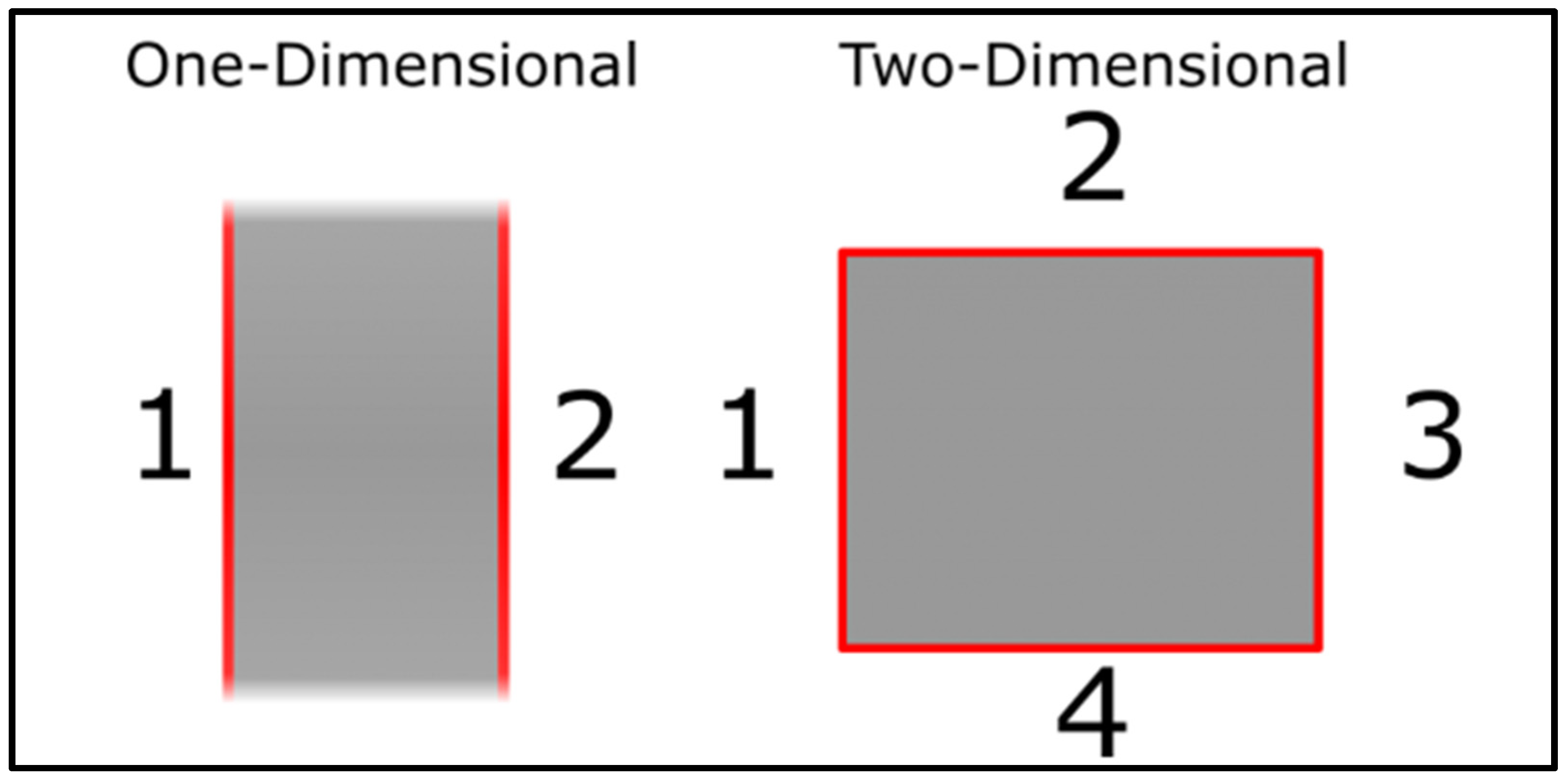
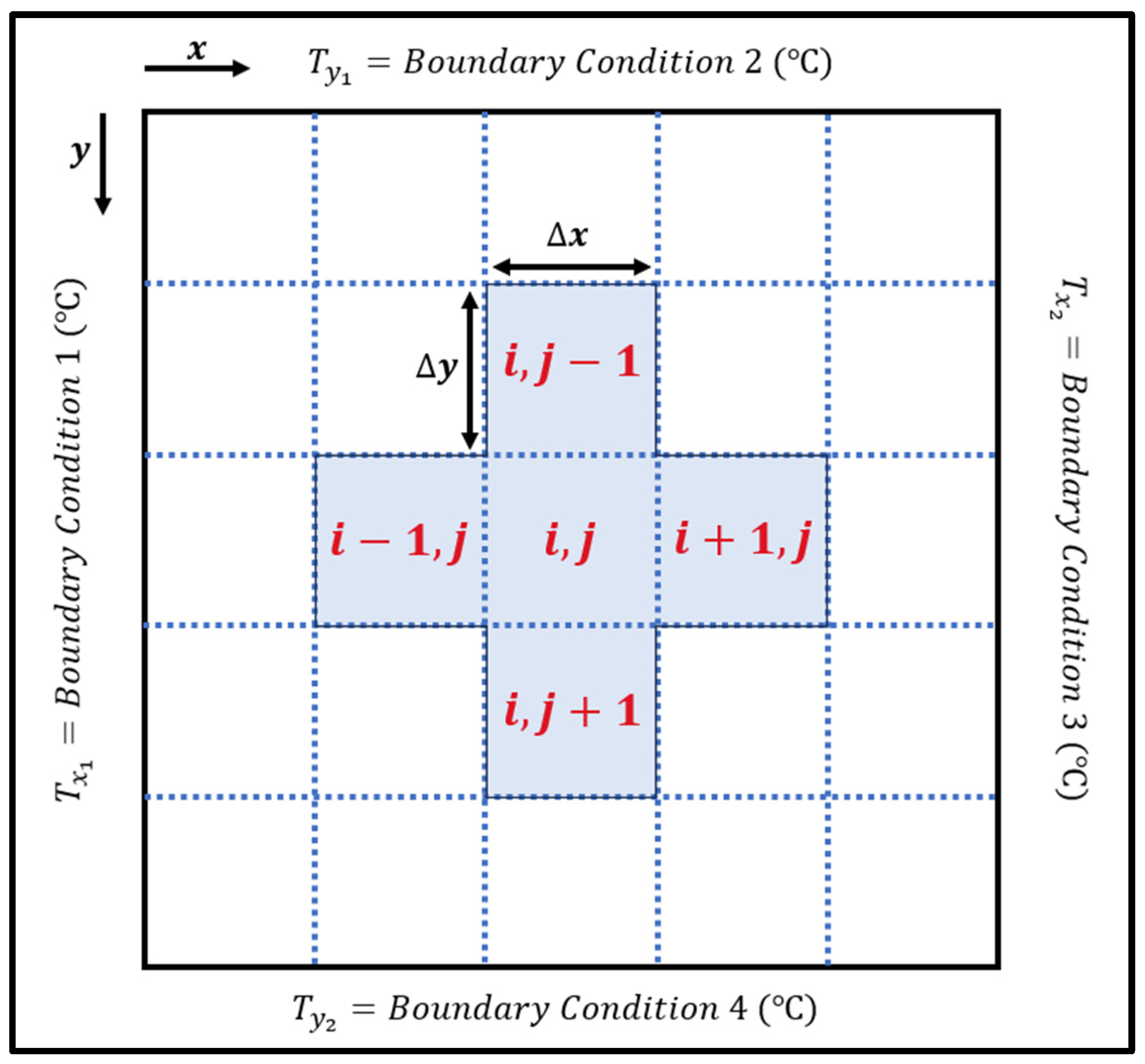
Heat transfer occurs between materials in different states—solid, liquid, and gas—from regions of high temperature to those of lower temperature through three primary modes: conduction, convection, and radiation. Conduction can happen in solids, liquids, and gases, involving direct contact where atoms from a high-temperature medium transfer kinetic energy to atoms in a cooler medium via vibrations. Convection, however, is limited to liquids and gases and requires movement within these mediums against a solid surface; the rate of heat transfer increases with the velocity of the moving fluid or gas. Radiation, uniquely, does not require a medium and can occur in a vacuum, transferring energy via electromagnetic waves at the speed of light, making it the fastest mode of heat transfer. In modeling heat transfer, one-dimensional (1D) simulations require two boundary conditions to depict temperature differences, whereas two-dimensional (2D) simulations need four, as seen in Figure 1. Heat transfer in any medium can occur through conduction, convection, or radiation, with steady-state conduction assuming constant temperature over time, and transient systems requiring initial conditions to determine temperature distribution [1].
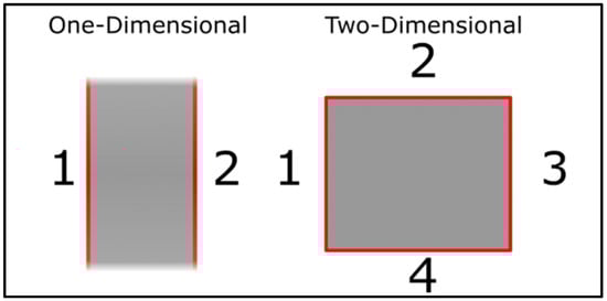
Figure 1.
Boundary conditions required in 1D and 2D heat transfer [1].
The main objective of measuring heat transfer is to quantify heating or cooling times within a medium and to visualize temperature variations. Various software tools, such as SimScale (v.2.0.0), COMSOL (v.6.2), MATLAB (2023b), and ANSYS (2023R2), are available to simulate heat transfer in mediums of different shapes and sizes with varying degrees of accuracy and customization. Simulating 2D heat transfer in irregular shapes aids in making informed design choices, potentially reducing prototyping costs, as materials and fabrication can be expensive. The accuracy of these simulations can differ from physical tests due to external factors like humidity, ambient temperature, and manufacturing defects. Therefore, accurate boundary and initial conditions in simulation software are essential to minimize discrepancies between simulated results and physical testing outcomes, ultimately optimizing heat transfer system designs.
2. Literature Review
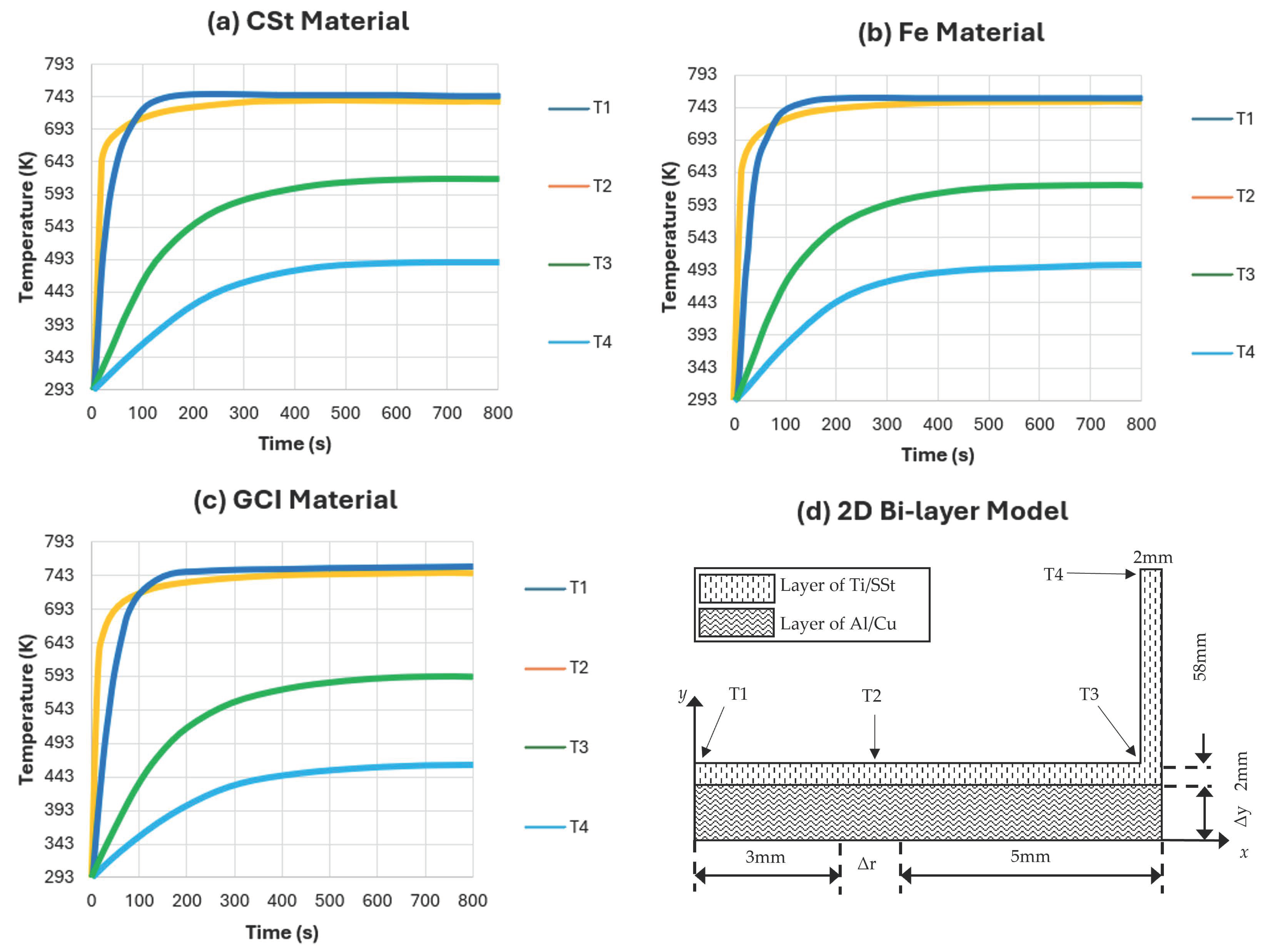
Studies of heat transfer on irregular shapes have significantly influenced design choices across various applications, such as in the development of frying pans. Irregular shapes are shapes that do not have equal angles or equal sides such as triangle/squares but a combination of different regular shapes. A notable example involves conducting a 2D heat transfer analysis on circular frying pans made from different materials using the Finite Element Method (FEM) within the ANSYS software. This analysis aimed to determine the temperature distribution on the top surface of both single-layer and multi-layer plate (MLP) frying pans. The study focused on materials like Carbon Steel (CSt), Iron (Fe), and Grey Cast Iron (GCI) within a circular shape, and the resulting temperature distributions are illustrated in Figure 2. To facilitate a clearer understanding, points T1–T4, which represent specific locations on the frying pan, are highlighted in Figure 2d and correspond to the temperature distributions shown in Figure 2a–c [2]. These detailed analyses help designers optimize material selection and structural design to achieve uniform heating, enhancing the performance and efficiency of frying pans.

Figure 2.
Plot of temperature against time for frying pans of different materials. (a) CSt material. (b) Fe material. (c) GCI material. (d) 2D bi-layer model in numerical analysis and positions of different selected nodes [2].
The ∆r as shown in Figure 2d is the thickness of the material which is 10 mm for GCI, CSt, and Fe. In reference [2], it states that “As we want to model irregularly heating, we constrained annular part of bottom side of pan”, and this is illustrated in Figure 2d, as ∆r, with a constant temperature of about 773 (K). There is a geometrical symmetry so the temperature gradients at the center of the plate along the y-axis have zero value. The side of the pan has convection heat transfer with air at ambient temperature. We have taken the thickness of layers according to Table 1, as shown below, whereby the thickness values for different materials are shown explicitly. This is because we are only using their CSt, Fe, and GCI test results, and all thicknesses are stated as 10 mm in this paper.

Table 1.
Symbol and thickness of the metals.
As illustrated in Figure 2a–c, the graph shows a gradient that ceases to increase and approaches a steady state at the 800 s mark, emphasizing the importance of simulating 2D steady-state conduction heat transfer. According to reference [2], single layer pans are worse than multi-layer pans due to the poorer temperature distribution. If we compare between the results of MLP vs SLP, it can be observed that MLP reaches a steady state a lot faster and has much better temperature distribution as compared to SLP. Hence, this justifies the steady-state simulations.
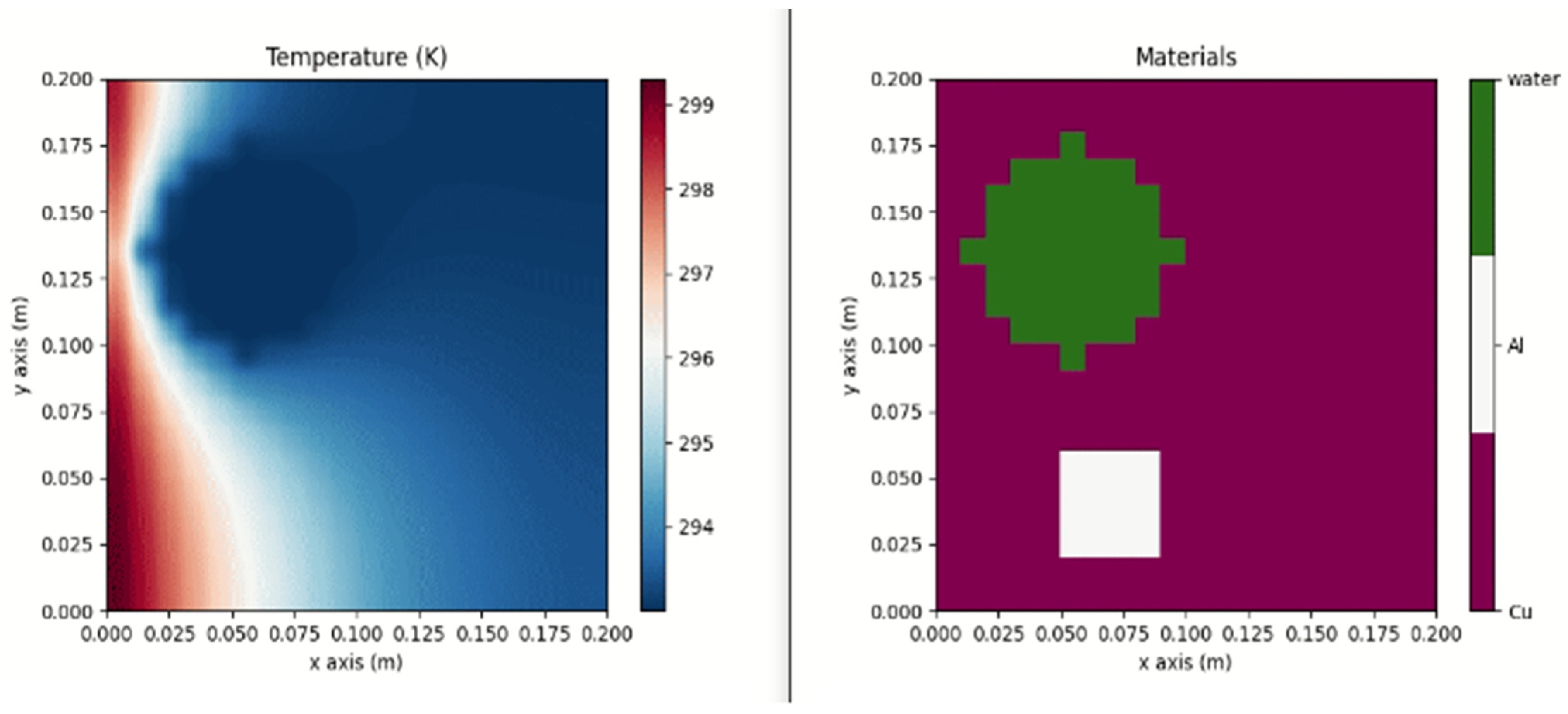
Such simulations reveal which frying pan materials can reach the desired temperature faster and maintain higher or lower temperatures, depending on the material. Python (v.3.12) offers multiple libraries capable of producing similar results to those provided by other software like MATLAB. As an open-source platform, Python has user-created libraries that can simulate 2D heat transfer, such as Heatrapy. This library supports simulating 1D and 2D heat transfer processes in solids using finite difference methods and can generate 2D plots based on parameters like temperature, material, heat power source, and state, as demonstrated in Figure 3. However, the Heatrapy database is limited to a few materials, including aluminum, copper, gadolinium, MnFePSi alloy, silica, vacuum, and water. Such tools are crucial for understanding and optimizing material performance in applications like frying pans, where material choice impacts the rate of heating and temperature retention.
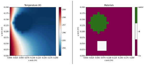
Figure 3.
Plot of 2D Heat Transfer using Heatrapy Python Library [3].
SciPy and NumPy are two essential Python libraries commonly used to solve Gauss–Seidel iterations. NumPy is particularly valuable due to its ability to index and vectorize n-dimensional arrays, which significantly aids in multigrid Gauss–Seidel iterations [4]. SciPy extends NumPy’s capabilities by providing tools for optimization, integration, interpolation, and solving complex mathematical problems such as eigenvalue problems, algebraic equations, and differential equations [5]. When combined, these libraries enable the creation of a universal code to perform Gauss–Seidel iterations using a full multigrid method, allowing for the simulation of 2D conduction heat transfer in materials with irregular shapes. Once the computational data are processed and stored in matrix form, the Matplotlib library can be employed to visualize the results as contour plots [6]. These plots, generated by the Python script, will be validated and benchmarked against ANSYS, a versatile software extensively used in engineering for various analyses, including Computational Fluid Dynamics (CFD) and Finite Element Analysis (FEA) [7]. ANSYS provides advanced solvers for both transient and steady-state thermal problems and includes an integrated Computer-Aided Design (CAD) feature, making it highly relevant for projects that require simulating 2D steady-state conduction heat transfer in irregular shapes within a square domain. By comparing the results from the Python-generated universal code with those from ANSYS, which relies on multiple user-defined equations and boundary conditions, the accuracy and reliability of the simulations can be ensured, ultimately leading to more precise and effective heat transfer analyses.
3. Proposed Theoretical Derivation
3.1. Numerical Solution
The numerical solution for steady heat conduction in plane walls can be derived from the energy balance equation in Equation (1) and simplified into Fourier’s law of heat conduction in Equation (2) [8].
- Energy Balance Equation:
The general form of the energy balance equation is given by the following:
For steady-state conditions, the rate of change for the energy in the wall is zero:
Therefore,
- 2.
- Fourier’s Law of Heat Conduction:
Fourier’s law in one dimension states that the heat transfer rate (Q) is proportional to the negative gradient of temperature and the area through which heat is conducted:
Here, k is the thermal conductivity, A is the cross-sectional area, and is the temperature gradient in the x-direction.
- 3.
- Derivation of Equation (2):
Consider a small element of the wall of thickness and the temperature difference across this element as T1−T2. By integrating Fourier’s law over the thickness (), and since the temperature gradient is assumed to be constant over , the integral simplifies to the following:
This explains how the result in Equation (2) is achieved through the integration of Fourier’s law of heat conduction. This integral accounts for the temperature gradient across the thickness of the wall, leading to the final form of the equation.
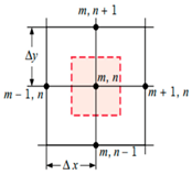
In 2D heat conduction at steady state conditions, once the four boundary conditions have been defined, the medium undergoing heat transfer is split into multiple control volumes also known as nodes, as shown in Figure 4.
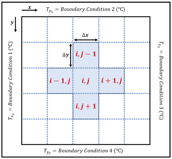
Figure 4.
Diagram for solving 2D heat conduction.
This method of solving 2D heat conduction uses an Excel solver to obtain the temperatures across a square-shaped medium assuming that the thermal conductivity of the medium, , is constant throughout [9]. The equation to derive heat transfer in 2D can be obtained by applying Equation (2) in Full Multigrid as shown in Equation (3) for the x-direction and in Equation (4) for the y-direction.
In the x-direction, it is as follows:
In the y-direction, it is as follows:
Therefore, in one node, combining both Equations (3) and (4) would produce Equation (5) under steady-state conditions. Equation (5) is to show the final combination of the two equations below. It is to find the temperature value in node i, j in both x and y directions.
The T values of each node can be determined to produce a contour plot which represents the temperature distribution within the medium using various iterative methods. However, it should be noted that this example only shows that of a square-shaped medium.
By going with the Gauss–Seidel iteration method, the Laplacian equation as shown in Equation (6) can be used to solve for steady-state heat conduction [10].
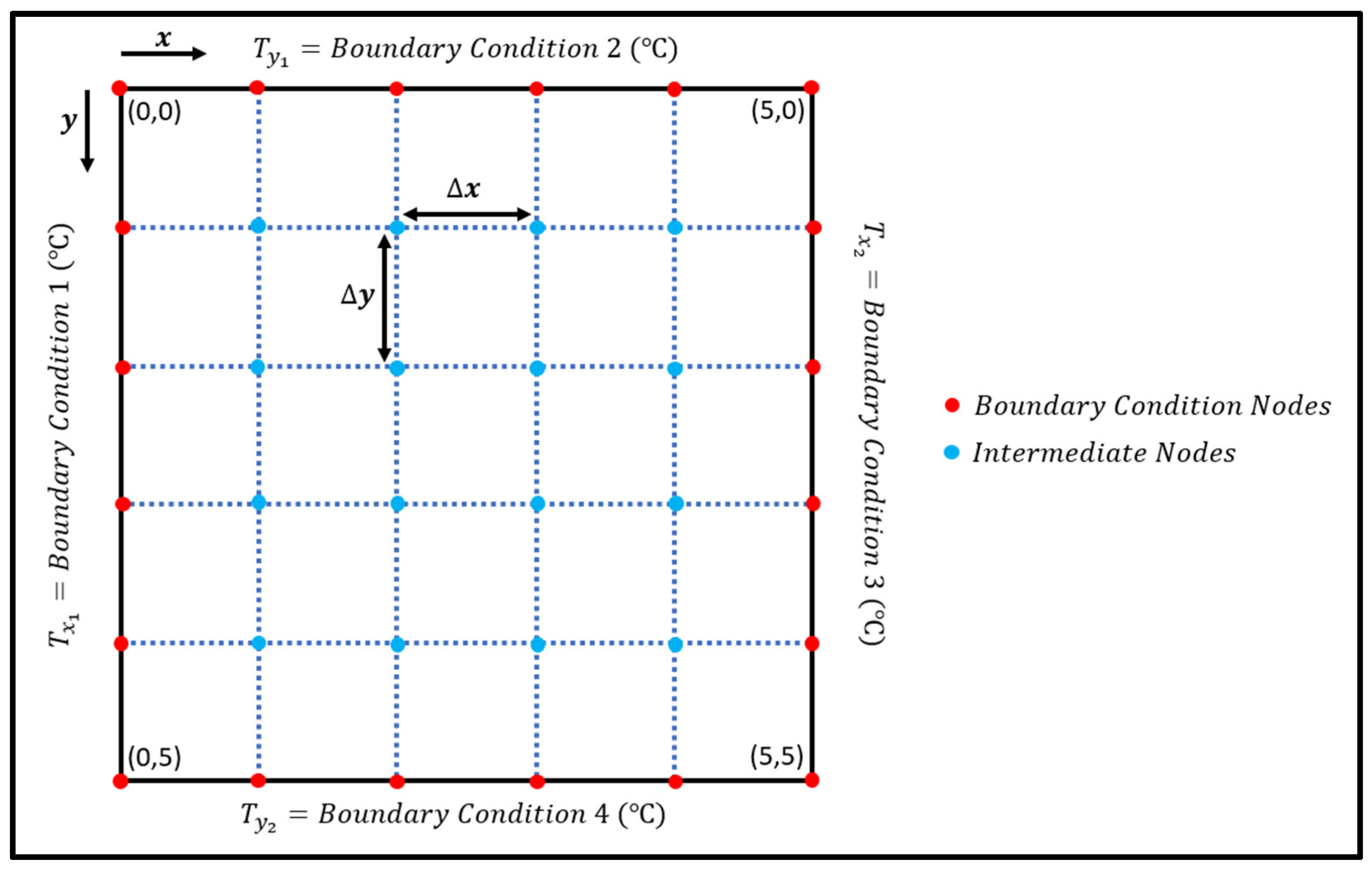
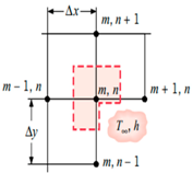
Due to the steady-state conditions, . Since , with reference to Figure 4, the energy that enters and leaves the node in the x and y direction, respectively, equals to 0. Hence, Equations (5) and (6) should be equal to zero. The Laplacian equation can be further expanded to Equation (7) using the central difference approximation to solve the T values of each node once each of the boundary condition nodes are determined as shown in Figure 5.
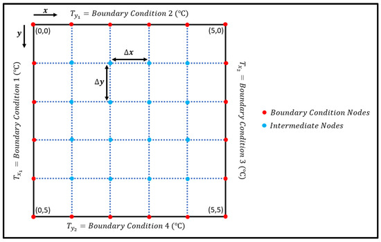
Figure 5.
Solving 2D heat conduction with Gauss–Seidel iteration.
With the boundary condition nodes predetermined depending on the scenario, Equation (7) can be further simplified into Equation (8) to solve for the T values at each node.
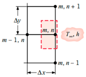
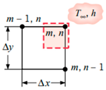
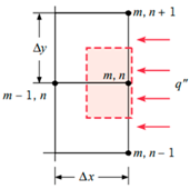
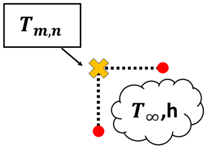
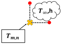
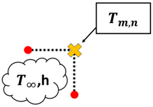
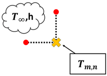
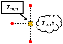
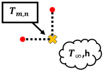
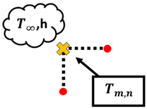
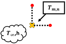
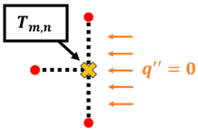
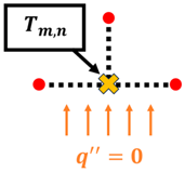
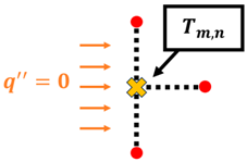
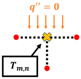
Once the T values of each node are obtained, the whole process is repeated until the maximum error of iteration n and n − 1 of is less than 0.0001 °C. Once the maximum error is within the tolerance set in place, the T values obtained have passed the convergence test. However, it should be noted that Equation (8) only applies to nodes that are strictly undergoing conduction only, such as interior nodes. Based on the summary of nodal finite-difference equations as shown in Table 2, different nodes within the 2D irregular shape have different equations with reference to what they are exposed to [11]. These equations are required to simulate 2D heat transfer [12,13,14,15,16,17,18] for materials of irregular shapes. A diagram of the nodal configurations is shown as well to further illustrate the equations involved. Note that to prevent confusion and to allow better understanding, the i and j subscripts have been changed to m and n subscripts, respectively.
Table 2.
Summary of nodal finite-difference equations [11].
Based on the equations shown in Table 1, the temperature value of the nodes, , can be obtained via rearranging the equation such that is now the subject. It should be noted that k is the thermal conductivity of the chosen material, h is the convection heat transfer coefficient and is the ambient temperature.
Interior node:
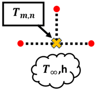
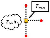
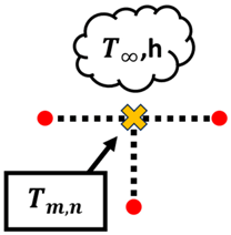
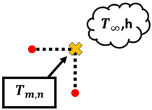
Node at an internal corner with convection:
Node at a plane surface with convection:
Node at an external corner with convection:
Node at a plane surface with insulation or surface of symmetry:
It should be noted that Equations (10)–(13) require manipulation to consider the different possible orientations of each respective node.
3.2. Analytical Solution
To simulate 2D heat transfer or irregular shapes via Gauss–Seidel iterations [19,20,21,22,23,24,25], a prior testing of applying Equation (14) within a script or Excel against a regular shape such as a square is required to ensure that results are accurate. To do so, an analytical solution is produced via Excel initially by implementing Equation (14) with reference to Figure 6 for a visualisation of how it is applied. This analytical solution provides the exact solution for a given square boundary which can then be compared with the numerical solution [26] obtained via the script produced.
whereby
- x and y are coordinate points with reference to nodes;
- W is the width of the boundary condition;
- L is the length of the boundary condition.
Equation (14) is valid, as the summation from one to infinity suggests a series solution rather than numerical integration. The correct approach involves solving the differential equation analytically rather than numerically integrating the series. Here is our explanation:
Equation (14) below represents an analytical solution for the temperature distribution in a rectangular domain using a Fourier series. Furthermore,
- is the dimensionless temperature variable;
- x and y are in meters (m);
- L and W are in meters (m).
The solution is achieved through the summation of the series, but for practical research purposes, a finite number of terms is used. Numerical integration is not appropriate here; rather, the series is truncated to a reasonable number of terms to approximate the solution. The summation should be correctly handled by truncating the series after enough terms to ensure accuracy without resorting to a numerical integration of the differential equation.
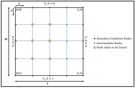
Figure 6.
Visualization of the analytical solution.
Figure 6.
Visualization of the analytical solution.
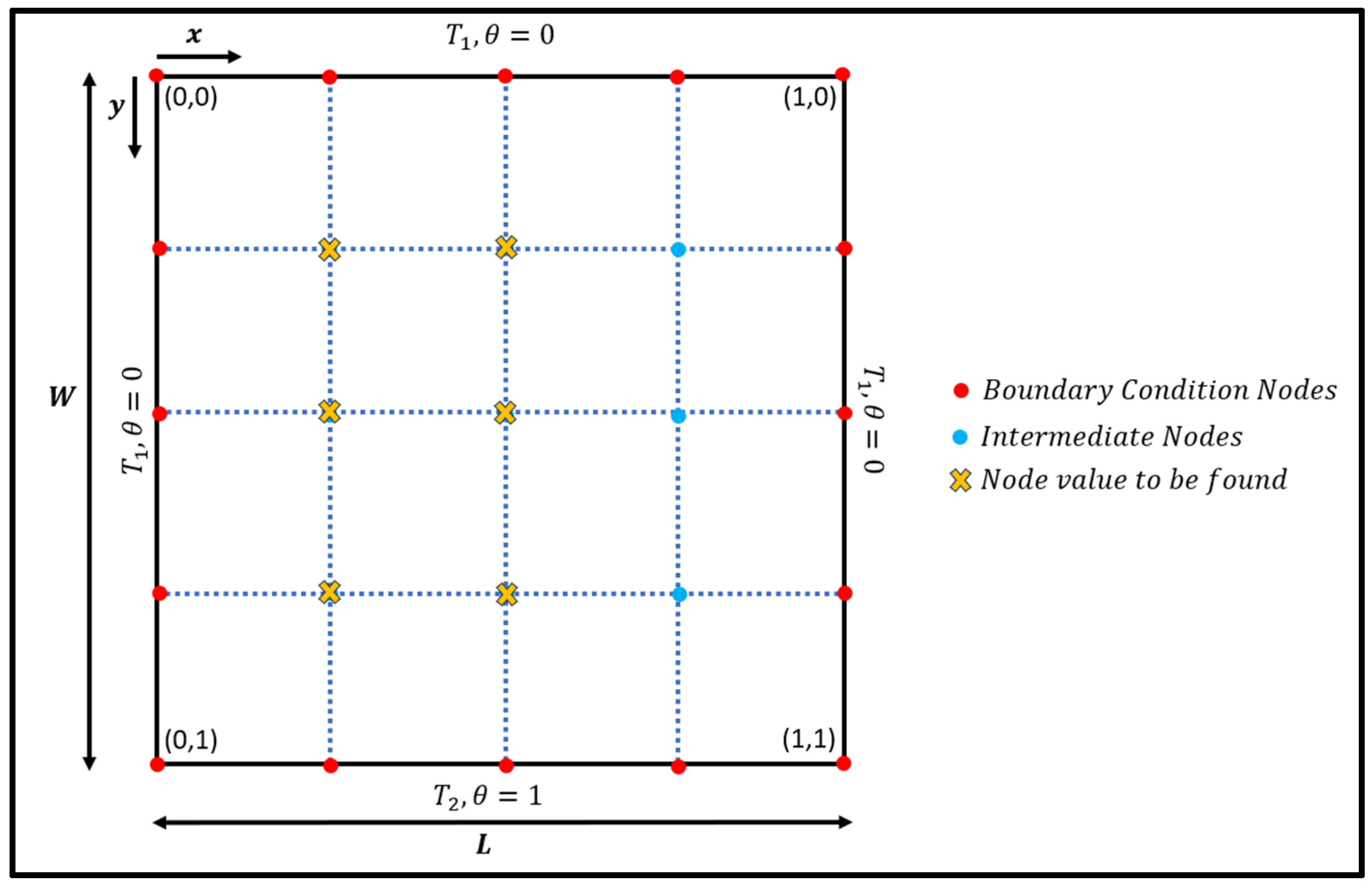
As Equation (14) will be tested on a square domain, nodes indicated with a yellow ‘x’ in the middle and left of the square domain as shown in Figure 6 are the ones that will have their values calculated as they mirror the nodes on the right-hand side. From the values obtained, Equation (15) can be used to find the temperature values at the respective nodes.
Equation (15) is derived from the temperature distribution equation.
Equation (15) aims to express the temperature TXY at a specific node in terms of a dimensionless temperature variable θ. This is based on the temperature distribution analysis within a given boundary. Furthermore, Equation (15) also shows that θ is a dimensionless quantity as it represents the normalized temperature difference. We have clarified that Equation (15) does not add different physical quantities. Instead, it multiplies the dimensionless temperature θ by the temperature difference T2-T1 (which has the units of temperature), and then adds the reference temperature T1 (which also has the units of temperature). The entire expression remains dimensionally consistent and results in a temperature value. Therefore, Equation (15) correctly combines the dimensionless temperature variable with temperature differences to yield a temperature value at a specific node, maintaining the consistency of physical units throughout the calculation. Theta (θ) is related to temperature distribution during the analysis of 2D heat transfer in irregular shapes. It is a dimensionless temperature variable used in the analytical solution of the temperature distribution equation. The relationship between theta (θ) and temperature is given by the following equation:
where
- Txy is the temperature at a specific node;
- T1 is the reference temperature (usually the initial temperature or the temperature at one boundary);
- T2 is the temperature at the other boundary;
- θ is the dimensionless temperature at the node of interest.
With the T values obtained, the results will be compared with the numerical solutions produced by the script. Ideally, the temperature value of the node at the middle of the square domain should be the same as the numerical solutions produced via the script. Temperature values of nodes surrounding the middle node should vary only slightly.
4. Proposed Work
4.1. Comparison between Analytical and Numerical Solution
To ensure that the code produced is accurate and functional, it is necessary to compare the results produced from the analytical solution via Excel against the solution produced from the numerical solution in Python [27,28,29]. This accuracy test can be conducted on a mesh size of as the results for varying mesh size are scalable in the form of . The accuracy of the universal code is validated only when the results produced in Excel match the results produced in Python for the same mesh size.
4.2. Mesh Size Optimization
To obtain the optimum mesh size, a comparison between the time taken and number of iterations required to reach the solution for the respective mesh sizes needs to be conducted. The mesh sizes of 9, 17, 33, 65, 129, 257, and 513 have been shortlisted to provide a more accurate representation of how mesh size will affect the time and number of iterations taken. The universal code will first be produced and tested against a regular square shape with the following boundary conditions with reference to Figure 6:
- W = 1;
- L = 1;
- T1 = 500 °C;
- T2 = 300 °C.
This is done to ensure that the code is fully functional and accurate prior to manipulating the array to implement the irregular shapes that will be tested. A regular square shape with only interior nodes undergoing insulation as shown in Equation (9) is chosen along with the abovementioned boundary conditions as it will take a significantly faster time to process to deduce the mesh size to be fixed across all future testing.
4.3. Manipulation of Equations Based on Orientation of Nodes
Once the optimum mesh sizes have been decided for all future testing and the results have been validated between the analytical and numerical solutions, all of the other equations listed in Table 1 can proceed and be implemented into the universal code. It should be noted that Equations (9)–(13) only coincide with the configuration for the respective nodes in Table 2. Therefore, there is a need to manipulate the equation based on the required orientation of the respective nodes. There is no need for the manipulation of Equation (9) as the calculation for an interior node considers all four directions before obtaining the values. Table 3, Table 4, Table 5 and Table 6 show the equations for the respective nodes manipulated to take into account the various orientations possible.
Table 3.
Equations for nodes at internal corners with convection in different orientations.
Table 4.
Equations for nodes at a plane surface with convection of different orientations.
Table 5.
Equations for nodes at external corners with convection in different orientations.
Table 6.
Equations for plane nodes with insulation or surface of symmetry in different orientations.
4.4. Utilization of Excel to Produce Irregular Shapes
To produce irregular shapes with ease, Microsoft Excel (v.16) was used to produce a 2D array. This will help with the visualization of the irregular shape and being able to identify the different nodes with varying nodal-finite difference equations. Table 7 shows the values keyed into the cells which correspond to the different node types with reference to Table 3, Table 4, Table 5 and Table 6.
Table 7.
Values keyed into the Excel file to correspond to the respective node types.
Python is able to read Excel files with the use of the Pandas library. This is shown in Listing 1. This allows Python to utilise the Numpy library to read the 2D array with all of the respective boundary conditions and nodes identified within the irregular shape.
Listing 1. Using Pandas library within Python to convert Excel data to a 2D array.
# Converting Excel into 2D Array for Python
DF = pd.DataFrame(pd.read_excel('ShapeDesigner.xlsx'))
df = DF.to_numpy()
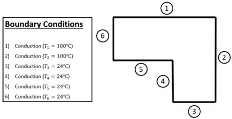
Figure 7 illustrates a scenario involving a steady-state 2D conduction heat transfer simulation [30,31] on an irregularly shaped object, defined by specific boundary conditions. To facilitate this simulation using the provided script, the required values must be input into an Excel sheet, as depicted on the right side of the figure. This Excel sheet corresponds to the boundary conditions outlined in Table 6. For clarity and ease of understanding, the mesh size in the Excel sheet shown is set to 17. This setup simplifies the process of translating the boundary conditions into the Excel format necessary for the script to run the simulation accurately. The mesh size and the detailed input values ensure that the simulation can handle the complexities of the irregular shape while maintaining precision in the conduction heat transfer analysis.
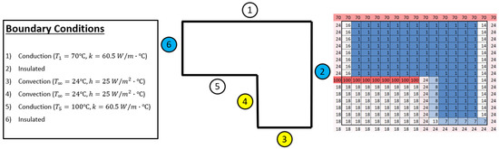
Figure 7.
Irregularly shaped object with different boundary conditions represented in Excel model designer.
In Figure 7, the boundary conditions outlined in Table 6 are translated into corresponding cell values in an Excel sheet. For instance, insulation requirements at planes 6 and 2 are indicated by assigning cell values of ‘16’ and ‘14’ to represent insulated nodes oriented to the west and east, respectively. Convection planes occurring at planes 3 and 4 are denoted by cell values of ‘7’7’, ‘8’, and ‘1’13’. Cell values of ‘1’ signify conduction throughout the entire irregular object and at planes 1 and 5. According to the boundary condition 1 and 5, it is under conduction conditions. The boundary condition (1) and (5) are set by us as observed in Figure 7. It is crucial to note that external and internal corner convection nodes are utilized only when two plane convection nodes intersect. Any redundant nodes should be assigned cell values of ‘18’8’ to eliminate them before plotting on the contour plot, ensuring a clearer representation of the irregular shape. This detailed mapping of boundary conditions to Excel cells ensures accuracy and clarity in the simulation process, facilitating a more precise analysis of 2D conduction heat transfer on complex geometries.
4.5. Execution of Python Script
The Python script is required to perform the following tasks:
- Convert the Excel file into a readable 2D array for Python.
- Have a timer that starts once the script is executed and stops after the Gauss–Seidel iterations have been completed.
- Find all of the indexes of where the respective nodes in Table 6 are located in the 2D array converted from the Excel file.
- Repeatedly perform the specified equations for the respective nodes that have been identified.
- Use a Gauss–seidel iteration to obtain the results for 2D steady-state conduction heat transfer of irregular shapes with various boundary conditions.
- Produce the contour plot of the results obtained to show the heat spread within the irregular shape at steady-state.
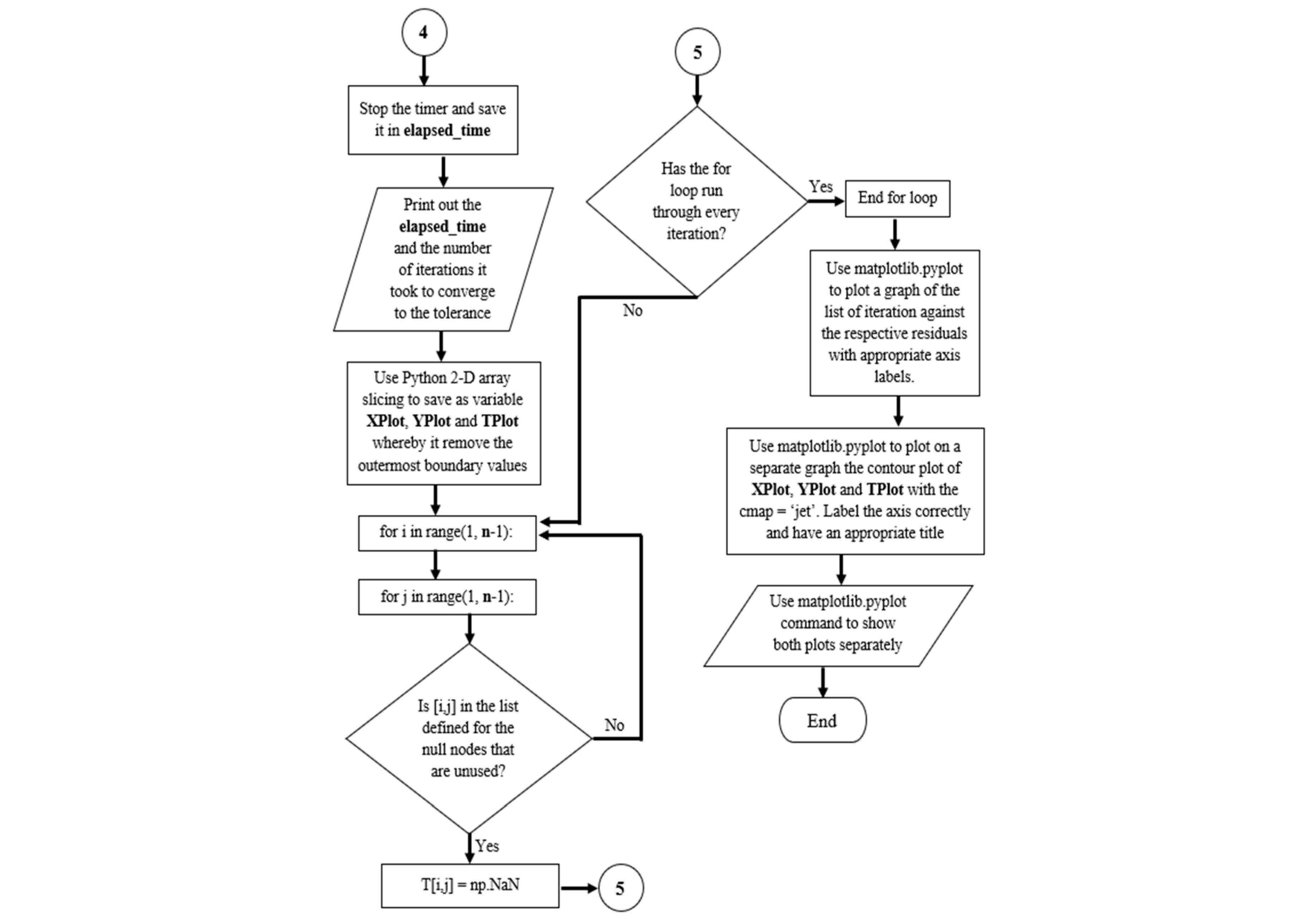
- The flowchart which elaborates on the entire process of the Python script used is shown below in Figure 8. The Python script used can be found in Appendix A.
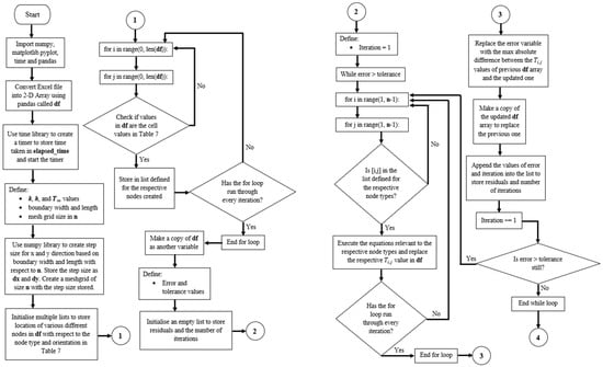
 Figure 8. Flowchart of Python script.
4.6. Use of Ansys to Validate Python Simulation
Within the Ansys software there are multiple different analysis systems that can be used. To validate the results produced via the Python script, the ‘Steady-State Thermal’ analysis system within the software can be used as it is capable of allocating temperature, convection, radiation, and insulation within the boundary of any shape or material.
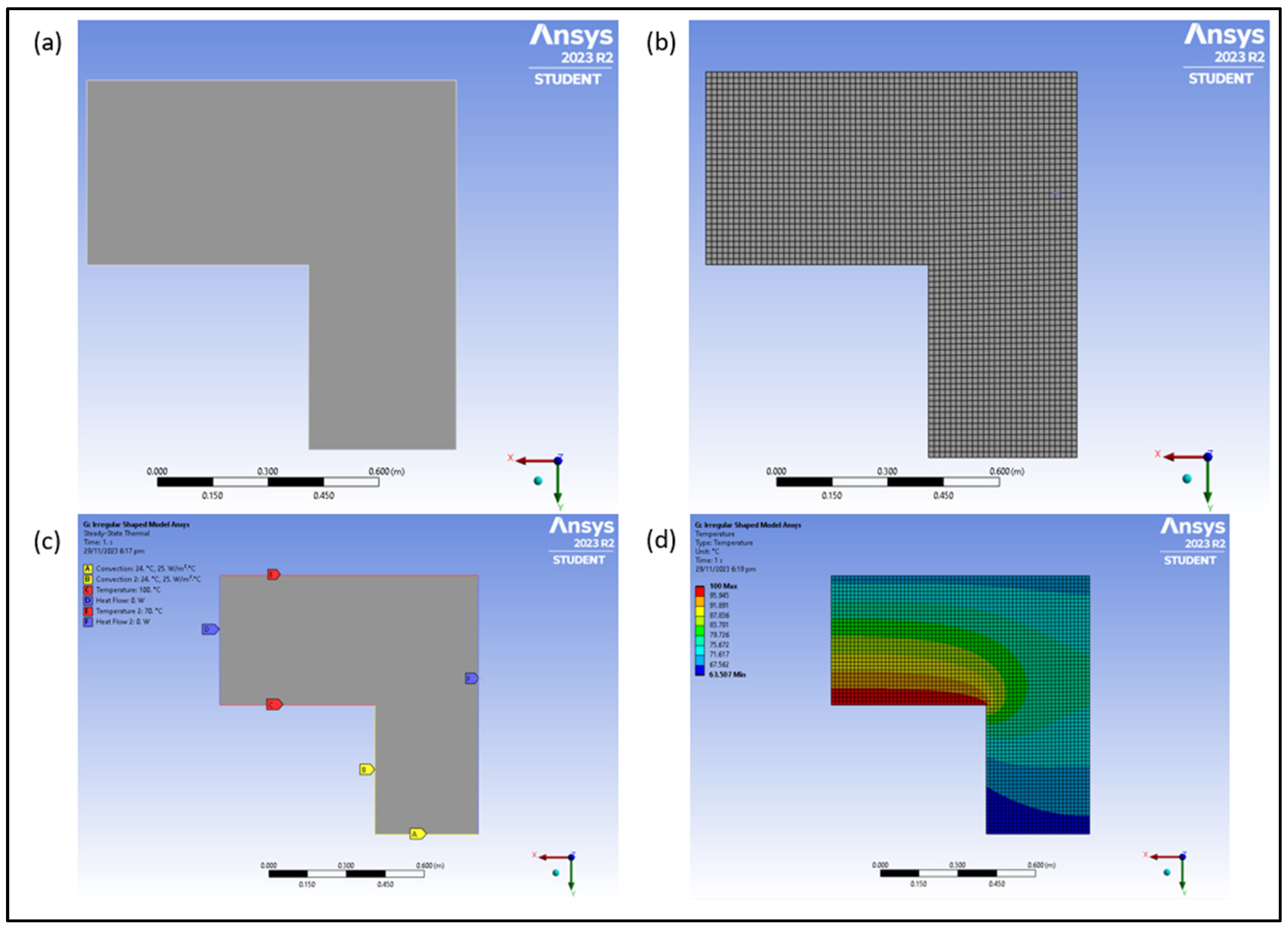
Figure 9a shows the shape chosen for validating the Python simulation. This irregular shape object is chosen as it can test all of the different node types listed in Table 6. The material selected to be tested will be structural steel with an h value of 25 W/(m2⋅°C) and k value of 60.5 W/(m⋅°C) as provided within the Ansys GRANTA Edupack software [1]. We provided a value for the convective heat transfer coefficient for structural steel, indicating its use in their simulations. This might lead to the misunderstanding that the convective heat transfer coefficient is a property of the material. However, it is important to clarify that the convective heat transfer coefficient is not an intrinsic property of the material like thermal conductivity or density. Instead, it is a parameter that depends on the conditions of the convective environment, such as the nature of the fluid, the flow conditions (laminar or turbulent), and the temperature difference between the surface and the fluid. In our study, a specific value for the convective heat transfer coefficient (25 W/m²·°C) was used for structural steel under conditions appropriate for performing the simulations accurately. This value was derived from experimental data or literature specific to the conditions under which the steel was used. After the irregularly shaped design has been modelled, face meshing and sizing have been applied to replicate that of the Excel file and how the nodes are represented within. Figure 9b shows the mesh produced with an element size of 0.015 m. The element size of 0.015 m has been chosen as the and values within the Python script which represents the element size of the model is 0.015 m as well. Allocating the various boundary conditions on the irregularly shaped model is shown in Figure 9c with reference to the scenario in Figure 7. To test the full functionality of the Python script, cell values listed in Table 6 with reference to the respective node type will need to be tested. As there are 18 different types of nodes with different equations, it is quintessential to ensure that all 18 are functioning correctly. To test all 18 types of nodes, various boundary conditions will be applied to the irregular shape. This can include conduction, convection, insulation and corner nodes on the north, south, east and west orientations, respectively. Figure 9d shows an example of such results with reference to the boundary conditions shown in Figure 9c.

Figure 9.
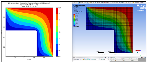
Irregularly shaped model to be tested in Ansys. (a) Model drawing. (b) Meshing applied on model. (c) Model with various boundary conditions applied. (d) Contour plot of model.
Such results produced via Ansys will be compared with the results obtained from the Python script. Ideally, the similarities between both should be very high especially in terms of the contour plot. Should the results be similar, it can be deduced that the Python script is accurate and can be relied upon.
5. Measured Results
5.1. Validation Test between Analytical and Numerical Solution
Using the analytical solution method in Excel, the following temperature values shown in Table 8 were obtained based on the boundary condition whereby
- W = 1;
- L = 1;
- T1 = 500 °C;
- T2 = 300 °C;
- Mesh size is 5 × 5.
Table 8.
Analytical solutions obtained via Excel.
Table 8.
Analytical solutions obtained via Excel.
| T(x,y) in °C | ||
|---|---|---|
| (0,0) | (0.25,0) | (0.5,0) |
| (0,0.25) | 486.4 | 480.9 |
| (0,0.5) | 463.6 | 450 |
| (0,0.75) | 413.6 | 391.9 |
With the same boundary conditions, Table 9 shows the numerical solution produced in Python.
Table 9.
Numerical solutions obtained via Python.
Comparing between Table 8 and Table 9 it is observed that the difference is 0.7 between both. Hence, it can be deduced that the numerical solution is working correctly and will increase in accuracy with increments in mesh resolution. However, with an increment in mesh resolution, more processing time is required, and hence optimization is necessary to find the best time taken against the accuracy ratio of the results produced. Mesh resolution refers to the fineness or coarseness of the mesh used in numerical simulations. Increasing mesh resolution means using a finer mesh with more elements, which typically enhances the accuracy of the solution but also increases computational time and resources required. A summary of the comparison between the analytical and numerical solution is shown in Table 10. As observed in Table 8, Table 9 and Table 10, the (0,0), (0,0.25), (0,2.5), and (0,0.75) refer to the node value based on the coordinates system as seen in Figure 6.
Table 10.
Difference between analytical and numerical solutions.
5.2. Mesh Size Testing Results
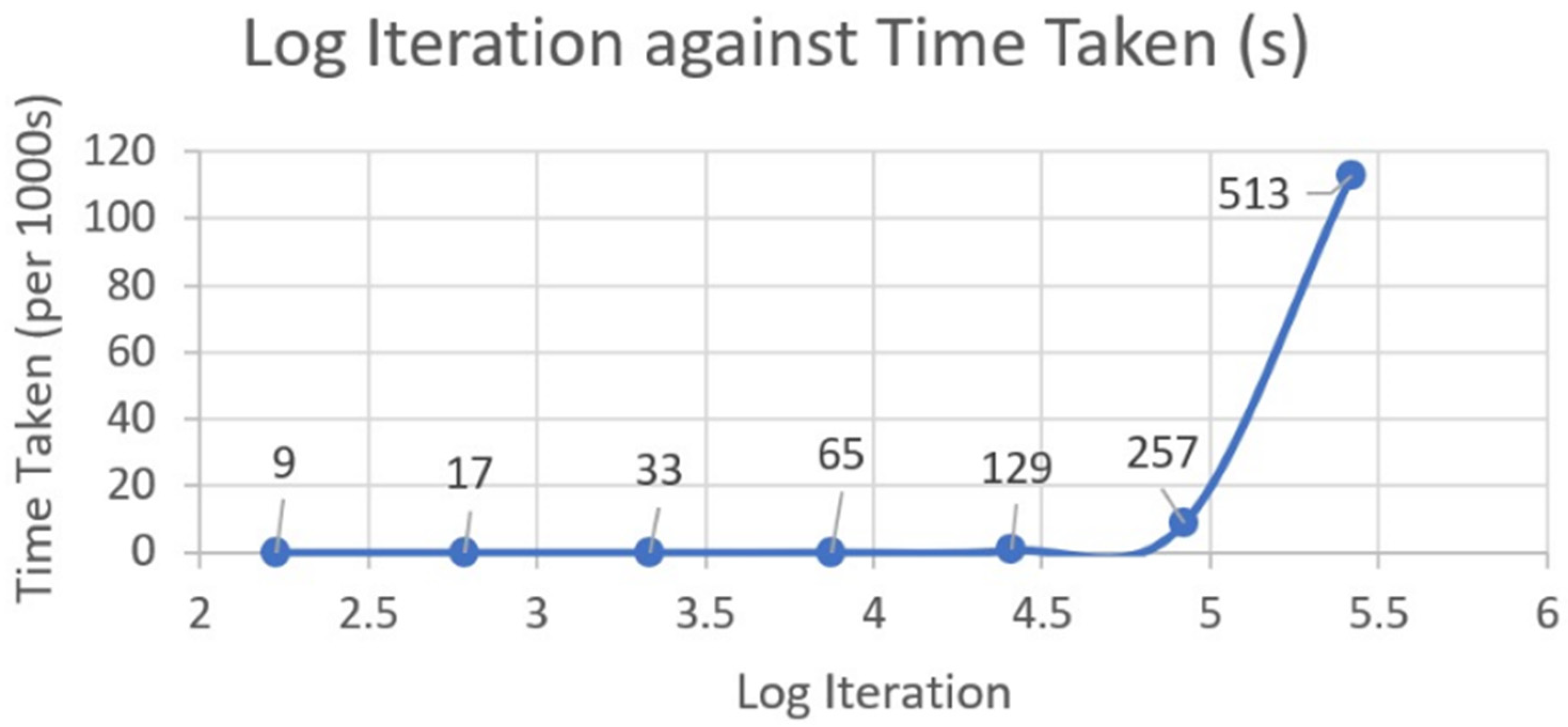
Table 11 shows the time taken and iterations needed before converging to a solution using the Python script based on mesh sizes of 9, 17, 33, 65, 129, 257, and 513 with the same aforementioned boundary conditions. The recorded number of iterations needed is expressed as a logarithmic function as shown in Figure 10.
Table 11.
Iterations needed against time taken for varying mesh sizes.
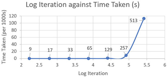
Figure 10.
Plot of log iteration against time taken for different mesh sizes.
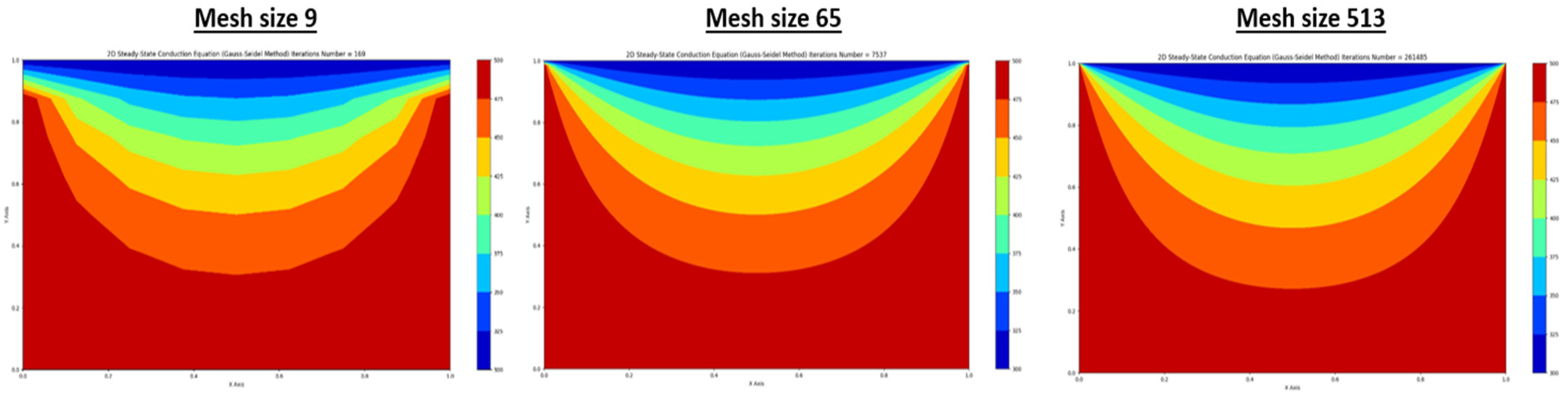
In Figure 10, a noticeable trend emerges revealing a significant rise in convergence time as the mesh size surpasses 129. Opting for a mesh size of 129 or higher promises heightened accuracy, particularly when time constraints are lenient, though at the expense of increased computational duration. For expedited solutions, a mesh size of 65 proves optimal, consuming a mere 50 s compared to the considerably longer 684 s required for larger mesh sizes. Figure 11 corroborates these findings by showcasing distinct disparities in contour plots generated across varying mesh sizes, highlighting the enhanced precision achieved as temperature gradient lines exhibit smoother convergence towards the intended corners. Notably, the discrepancy between contour plots generated by mesh sizes of 65 and 513 is marginal, rendering the additional computational overhead unjustifiable. Consequently, a mesh size of 65 is determined as the most efficient choice going forward, striking a balance between accuracy and computational efficiency. For better clarity for Figure 11, you can refer to the following:
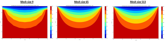
Figure 11.
Comparison of contour plot produced for different mesh sizes.
Mesh Size 9, Header: 20 Steady-State Conduction Equation (Gauss–Seidel Method) Iterations Number = 169.
Mesh Size 65, Header: 20 Steady-State Conduction Equation (Gauss–Seidel Method) Iterations Number = 7537.
Mesh Size 513, Header: 20 Steady-State Conduction Equation (Gauss–Seidel Method) Iterations Number = 261,485.
5.3. 2D Heat Transfer of Irregular Shapes Test
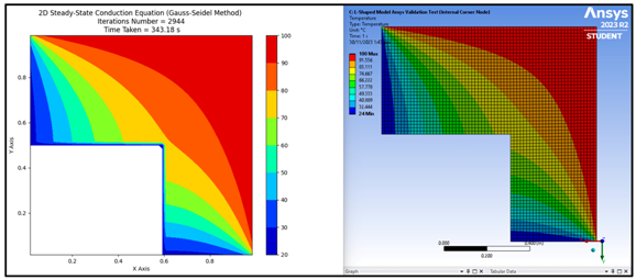
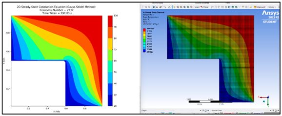
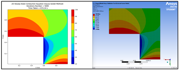
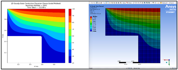
To test if the various node types as listed in Table 7 are functioning correctly, different boundary conditions will be implemented, and the results produced via the Python script will be validated against the results produced in Ansys. It should be noted that all tests conducted are done with a mesh size of , an h value of 25 W/m2⋅°C, and a k value of 60.5 W/m⋅°C is used as the material is assumed to be structural steel. These values were obtained from the materials database included within the Ansys GRANTA Edupack software [1]. All tests conducted in Ansys also use a mesh element size of 0.015 m to replicate the distance between each node in the Excel sheet. Table 12 shows the various nodal equations being tested in the Python script and compares them with the results produced in Ansys.
Table 12.
Summary of nodal testing conducted.
Furthermore, as shown in Table 12, the different rows refer to the different boundary condition shown below.
Row 1—Interior node (All six boundaries are conduction conditions):
Row 2—Interior corner node with convection (all boundaries are conduction except 4 and 5):
Row 3—Plane node with convection (all boundaries are conduction except 5):
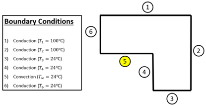
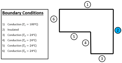
Row 4—External corner node with convection (all boundaries are conduction except 1, 2, and 6):
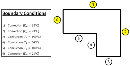
Row 5—Insulated node or surface of symmetry (all boundaries are conduction except 2 is insulated):
As shown in Table 12, the code is not limited to solving heat conduction only, it can be used for convection as well. As mentioned in the conclusion section, despite the disparities between the results in ANSYS and the code, it highlights the underlying limitations of the code. Hence, the similarities in results do outweigh the differences as the differences only occur on the boundaries where convection is applied. Through extensive nodal testing, it has been observed that all nodal equations integrated into the Python script function effectively, exhibiting a degree of accuracy comparable to results generated in Ansys simulations. Notably, as the number of boundary conditions increases in the Excel sheet, the Python script requires more iterations and time to complete the Gauss–Seidel iterations. Nevertheless, it stands as a viable alternative to other software for 2D steady-state conduction heat transfer of irregular shapes, given its accessibility as free and open-source software. The Python script demonstrates capability in simulating 2D steady-state conduction heat transfer on irregular shapes with diagonal lines by amalgamating various node types involving convection, as outlined in Table 6, to simulate diagonal boundary conditions where convection occurs. While the interior node equation suffices for conducting heat on diagonals, the script faces limitations in simulating insulated planes on diagonals due to constraints in Equation (13), applicable only to nodes aligned in straight horizontal or vertical lines. Notably, for testing conducted on irregular shapes with diagonal lines, material properties assumed for structural steel—specifically, an h value of 25 W/m² °C and a k value of 60.5 W/m °C—are utilized, sourced from the materials database within Ansys GRANTA Edupack software. The boundary conditions and results obtained to assess conduction on irregular shapes with diagonal lines are depicted in Figure 12a, alongside outcomes derived from both the Python script and Ansys simulations in Figure 12b.
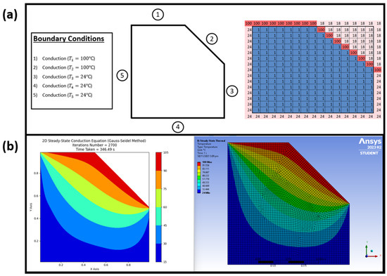
Figure 12.
Irregularly shaped model used to test for conduction on irregular shapes with diagonal lines. (a) Boundary conditions applied with simplified Excel model designer. (b) Comparison results produced between Python script and Ansys.
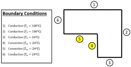
The boundary conditions and results produced to test for convection on irregular shapes with diagonal lines are shown in Figure 13a together with the results produced by the Python script and Ansys in Figure 13b.
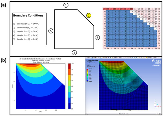
Figure 13.
Irregularly shaped model used to test for convection on irregular shapes with diagonal lines. (a) Boundary conditions applied with simplified Excel model designer. (b) Comparison results produced between Python script and Ansys.
5.4. Limitations
While the Python script effectively simulates 2D steady-state conduction heat transfer on irregular shapes [32,33], several limitations hinder its versatility. Firstly, boundary temperatures ranging from 1 °C to 18 °C cannot be utilized, as they serve as identifiers for node types in the Excel-generated 2D array processed by the script, although negative boundary temperatures are compatible. Additionally, Equation (13) and its variants are constrained to straight horizontal or vertical lines, rendering insulated planes on diagonal lines unattainable. Moreover, processing times surpass those of Ansys, albeit contingent upon the computational power of the utilized device; enhanced processor capabilities would expedite Gauss–Seidel iteration calculations. Excel-based shape sketching proves cumbersome compared to Ansys due to the manual input required for each node type referencing Table 6. While results from the Python script fall short of Ansys’ accuracy, adjusting the tolerance to a smaller value improves precision at the expense of increased processing time; at a tolerance of 0.0001, Python results closely resemble those of Ansys regarding heat distribution within irregular shapes. Future improvements could integrate machine learning [34,35,36] and artificial intelligence techniques [37,38] to enhance the simulation process further.
6. Conclusions
The introduction of this universal Python code for simulating 2D steady-state heat transfer on irregular shapes marks a significant advancement in democratizing access to advanced engineering simulations. It eliminates the need for costly software like ANSYS, COMSOL, and SimScale by using accessible tools such as Microsoft Excel and Python. This approach benefits educational institutions with limited resources, enhancing accessibility to heat transfer simulations. The code employs Gauss–Seidel iteration within a multigrid method and uses tailored nodal finite-difference equations for different node types in irregular shapes, making the simulation process clear and comprehensible. Excel’s use for visualization and data manipulation in Python increases ease of use, avoiding the need for complex diagram sketching techniques required by other software. Comparing contour plot results between the Python code and ANSYS demonstrates its accuracy, validating it as a simplified alternative for heat transfer simulations. This code not only reduces costs but also empowers students and educators with practical applications, fostering a deeper understanding of heat transfer principles.
Author Contributions
Conceptualization, Data Curation, Supervision, and Investigation, C.L.K.; Methodology, Resources and Software, Supervision, and Funding Acquisition, C.K.H.; Project administration, Investigation, Visualization, and Formal analysis, A.S.B.M.T.; Investigation, Supervision, and Funding Acquisition, Y.Y.K.; Conceptualization, Data Curation, Visualization, and Supervision, T.H.T. All authors have read and agreed to the published version of the manuscript.
Funding
This research received no external funding.
Data Availability Statement
The data presented in this study are available on request from the corresponding author.
Acknowledgments
The authors would like to extend their appreciation to the University of Newcastle, Australia, for financing the project.
Conflicts of Interest
The authors declare no conflicts of interest.
Appendix A
import numpy as np
import matplotlib.pyplot as plt
import time
import pandas as pd
# Converting Excel into 2D Array for Python
DF = pd.DataFrame(pd.read_excel('ShapeDesigner.xlsx'))
df = DF.to_numpy()
# Function to count duration taken to obtain results
def start_stopwatch():
return time.time()
def stop_stopwatch(start_time):
return time.time() - start_time
# Start recording time taken to complete process
start_time = start_stopwatch()
# Define k, h and ambient temperature (Tinf) values
k = 60.5 # for steel
h = 25 # for steel
Tinf = 24 # Ambient room temp
# Boundary Width and Length
W = 1
L = 1
# No. of Grids (mesh size must be 2n - 1) (513, 257, 129, 65, 33, 17, 9)
n = 65
# Step size in x and y directions
x = np.linspace(0, W, n)
y = np.linspace(L, 0, n)
dx = x[2] - x[1]
dy = y[2] - y[1]
X, Y = np.meshgrid(x, y)
# Initialization of boundary and matrix conditions
V = np.zeros([n, n])
T = V + df
# Internal Nodes with Conduction
Type1Nodes = []
# Internal Nodes with Convection
Type2Nodes_NW = []
Type2Nodes_SW = []
Type2Nodes_NE = []
Type2Nodes_SE = []
# Plane Node with Convection
Type3Nodes_E = []
Type3Nodes_S = []
Type3Nodes_W = []
Type3Nodes_N = []
# External bends with Convection
Type4Nodes_NE = []
Type4Nodes_SE = []
Type4Nodes_NW = []
Type4Nodes_SW = []
# For insulation planes and surface of symmetry
Type5Nodes_E = []
Type5Nodes_S = []
Type5Nodes_W = []
Type5Nodes_N = []
# To identify nodes to nullify for plotting purposes
TypeNANodes = []
# Storing location of each type of Node in 2D Array
for i in range(0, len(df)):
for j in range(0, len(df)):
if df[i, j] == 1:
Type1Nodes.append([i, j])
elif df[i, j] == 2:
Type2Nodes_NW.append([i, j])
elif df[i, j] == 3:
Type2Nodes_SW.append([i, j])
elif df[i, j] == 4:
Type2Nodes_NE.append([i, j])
elif df[i, j] == 5:
Type2Nodes_SE.append([i, j])
elif df[i, j] == 6:
Type3Nodes_E.append([i, j])
elif df[i, j] == 7:
Type3Nodes_S.append([i, j])
elif df[i, j] == 8:
Type3Nodes_W.append([i, j])
elif df[i, j] == 9:
Type3Nodes_N.append([i, j])
elif df[i, j] == 10:
Type4Nodes_NE.append([i, j])
elif df[i, j] == 11:
Type4Nodes_SE.append([i, j])
elif df[i, j] == 12:
Type4Nodes_NW.append([i, j])
elif df[i, j] == 13:
Type4Nodes_SW.append([i, j])
elif df[i, j] == 14:
Type5Nodes_E.append([i, j])
elif df[i, j] == 15:
Type5Nodes_S.append([i, j])
elif df[i, j] == 16:
Type5Nodes_W.append([i, j])
elif df[i, j] == 17:
Type5Nodes_N.append([i, j])
elif df[i, j] == 18:
TypeNANodes.append([i, j])
# Initialization for Gauss-Seidel Iteration
oldT = T.copy()
error = 1
tol = 1e-4
residual = []
iterationNo = []
# Execution Gauss-Seidel Iteration
iteration = 1
while error > tol:
for i in range(1, n-1):
for j in range(1, n-1):
if [i, j] in Type1Nodes:
T[i, j] = (T[i, j+1] + T[i, j-1] + T[i+1, j] + T[i-1, j]) / 4
elif [i, j] in Type2Nodes_NW:
T[i, j] = ((2 * (T[i, j - 1] + T[i - 1, j])) + (T[i, j + 1] + T[i + 1, j]) + (2 * ((h * dx) / k) * Tinf)) / (6 + ((2 * h * dx) / k))
elif [i, j] in Type2Nodes_SW:
T[i, j] = ((2 * (T[i + 1, j] + T[i, j - 1])) + (T[i - 1, j] + T[i, j + 1]) + (2 * ((h * dx) / k) * Tinf)) / (6 + ((2 * h * dx) / k))
elif [i, j] in Type2Nodes_NE:
T[i, j] = ((2 * (T[i - 1, j] + T[i, j + 1])) + (T[i + 1, j] + T[i, j - 1]) + (2 * ((h * dx) / k) * Tinf)) / (6 + ((2 * h * dx) / k))
elif [i, j] in Type2Nodes_SE:
T[i, j] = ((2 * (T[i, j + 1] + T[i + 1, j])) + (T[i, j - 1] + T[i - 1, j]) + (2 * ((h * dx) / k) * Tinf)) / (6 + ((2 * h * dx) / k))
elif [i, j] in Type3Nodes_E:
T[i, j] = ((2 * T[i, j - 1] + T[i + 1, j] + T[i - 1, j]) + ((2 * h * dx * Tinf) / k)) / (((2 * h * dx) / k) + 4)
elif [i, j] in Type3Nodes_S:
T[i, j] = ((2 * T[i - 1, j] + T[i, j - 1] + T[i, j + 1]) + ((2 * h * dx * Tinf) / k)) / (((2 * h * dx) / k) + 4)
elif [i, j] in Type3Nodes_W:
T[i, j] = ((2 * T[i, j + 1] + T[i + 1, j] + T[i - 1, j]) + ((2 * h * dx * Tinf) / k)) / (((2 * h * dx) / k) + 4)
elif [i, j] in Type3Nodes_N:
T[i, j] = ((2 * T[i + 1, j] + T[i, j + 1] + T[i, j - 1]) + ((2 * h * dx * Tinf) / k)) / (((2 * h * dx) / k) + 4)
elif [i, j] in Type4Nodes_NE:
T[i, j] = ((T[i + 1, j] + T[i, j - 1]) + ((2 * h * dx * Tinf) / k)) / (((2 * h * dx) / k) + 2)
elif [i, j] in Type4Nodes_SE:
T[i, j] = ((T[i - 1, j] + T[i, j - 1]) + ((2 * h * dx * Tinf) / k)) / (((2 * h * dx) / k) + 2)
elif [i, j] in Type4Nodes_NW:
T[i, j] = ((T[i + 1, j] + T[i, j + 1]) + ((2 * h * dx * Tinf) / k)) / (((2 * h * dx) / k) + 2)
elif [i, j] in Type4Nodes_SW:
T[i, j] = ((T[i - 1, j] + T[i, j + 1]) + ((2 * h * dx * Tinf) / k)) / (((2 * h * dx) / k) + 2)
elif [i, j] in Type5Nodes_E:
T[i, j] = ((2 * T[i, j - 1]) + T[i + 1, j] + T[i - 1, j]) / 4
elif [i, j] in Type5Nodes_S:
T[i, j] = ((2 * T[i - 1, j]) + T[i, j + 1] + T[i, j - 1]) / 4
elif [i, j] in Type5Nodes_W:
T[i, j] = ((2 * T[i, j + 1]) + T[i + 1, j] + T[i - 1, j]) / 4
elif [i, j] in Type5Nodes_N:
T[i, j] = ((2 * T[i + 1, j]) + T[i, j + 1] + T[i, j - 1]) / 4
error = np.max(np.abs(T-oldT))
oldT = T.copy()
iterationNo.append(iteration)
residual.append(error)
iteration = iteration + 1
# Stop counting the time taken to complete Gauss-Seidel Iteration and print results
elapsed_time = stop_stopwatch(start_time)
print("Script was completed with Iteration No.:", iteration, " and Elapsed Time:", elapsed_time, " s")
# Remove Temperature at boundary for cleaner contour plot
XPlot = X[1:-1, 1:-1]
YPlot = Y[1:-1, 1:-1]
TPlot = T[1:-1, 1:-1]
# Remove unused nodes from 2D array for cleaner contour plot
for i in range(1, n-1):
for j in range(1, n-1):
if [i, j] in TypeNANodes:
T[i, j] = np.NaN
else:
continue
# To plot residual against iteration number taken for solution to converge
plt.figure(1)
plt.plot(iterationNo, residual)
plt.xlabel('Iteration No.')
plt.ylabel('Residuals')
# To produce contour plot of 2D steady-state conduction heat transfer of irregular shape
plt.figure(2)
title = "2D Steady-State Conduction Equation (Gauss-Seidel Method) \n Iterations Number = {} \n Time Taken = {:.2f} s".format(iteration, elapsed_time)
plt.contourf(XPlot, YPlot, TPlot, cmap='jet')
plt.xlabel('X Axis')
plt.ylabel('Y Axis')
plt.colorbar()
plt.title(title)
plt.show()
References
- Qdot Systems. Boundary Conditions for the Heat Conduction Equation. Available online: https://qdotsystems.com.au/boundary-conditions-for-the-heat-conduction-equation/ (accessed on 23 May 2023).
- Dardashti, B.N.; Sedighi, M.R. Numerical Solution of Heat Transfer for Single and Multi-Metal Pan. Appl. Mech. Mater. 2011, 148–149, 227–231. [Google Scholar] [CrossRef]
- Silva, D. Heatrapy Source Code, Version 2.0.3. Available online: https://github.com/djsilva99/heatrapy/wiki (accessed on 3 June 2023).
- Harris, C.R.; Millman, K.J.; Van Der Walt, S.J.; Gommers, R.; Virtanen, P.; Cournapeau, D.; Wieser, E.; Taylor, J.; Berg, S.; Smith, N.J.; et al. Array programming with NumPy. Nature 2020, 585, 357–362. [Google Scholar] [CrossRef] [PubMed]
- Virtanen, P.; Gommers, R.; Oliphant, T.E.; Haberland, M.; Reddy, T.; Cournapeau, D.; Burovski, E.; Peterson, P.; Weckesser, W.; Bright, J.; et al. SciPy 1.0: Fundamental Algorithms for Scientific Computing in Python. Nat. Methods 2020, 17, 261–272. [Google Scholar] [CrossRef] [PubMed]
- Hunter, J.D. Matplotlib: A 2D graphics environment. Comput. Sci. Eng. 2007, 9, 90–95. [Google Scholar] [CrossRef]
- ANSYS Inc. Ansys GRANTA EduPack Software, Version 2023 R2. Available online: https://www.ansys.com/products/materials/granta-edupack (accessed on 10 October 2023).
- Cengel, Y.A.; Boles, M.A. Thermodynamics an Engineering Approach, 8th ed.; McGraw Hill: New York, NY, USA, 2015. [Google Scholar]
- Chisăliţă, G.-A.; Kapalo, P. Steady state two-dimensional heat conduction in a square cross section, by using Microsoft Excel® for numerical modeling. Rev. Romana Ing. Civila 2022, 13, 10–25. [Google Scholar] [CrossRef]
- Roy, A.K.; Kumar, K. 2D heat conduction on a flat plate with Ti6Al4V alloy under steady state conduction: A numerical analysis. Mater. Today Proc. 2021, 46, 896–902. [Google Scholar] [CrossRef]
- Incropera, F.P.; DeWitt, D.P.; Bergman, T.L.; Lavine, A.S. Fundamentals of Heat and Mass Transfer, 6th ed.; Wiley: Hoboken, NJ, USA, 2006. [Google Scholar]
- Tamma, K.K.; Namburu, R.R.; Ramesh, K.S. Computational Techniques for Heat Transfer and Fluid Flow Problems; Springer: Berlin/Heidelberg, Germany, 2004. [Google Scholar]
- Bartosik, A.S. Numerical Heat Transfer and Fluid Flow: New Advances. Energies 2023, 16, 5528. [Google Scholar] [CrossRef]
- Srinivasacharya, D.; Reddy, K.S. (Eds.) Numerical Heat Transfer and Fluid Flow: Select Proceedings of NHTFF 2018; Springer: Berlin/Heidelberg, Germany, 2019. [Google Scholar]
- Kok, C.L.; Chia, K.J.; Siek, L. A 87 dB SNR and THD+N 0.03% HiFi Grade Audio Preamplifier. Electronics 2024, 13, 118. [Google Scholar] [CrossRef]
- Versteeg, H.K.; Malalasekera, W. An Introduction to Computational Fluid Dynamics: The Finite Volume Method; Pearson Education: London, UK, 2007. [Google Scholar]
- Anderson, J.D. Computational Fluid Dynamics: The Basics with Applications; McGraw-Hill: New York, NY, USA, 1995. [Google Scholar]
- Bird, R.B.; Stewart, W.E.; Lightfoot, E.N. Transport Phenomena; John Wiley & Sons: Hoboken, NJ, USA, 2006. [Google Scholar]
- Langtangen, H.P. A Primer on Scientific Programming with Python; Springer: Berlin/Heidelberg, Germany, 2016. [Google Scholar]
- Oliphant, T.E. A Guide to NumPy; Trelgol Publishing: Provo, UT, USA, 2006. [Google Scholar]
- Downey, A.B. Think Python: How to Think like a Computer Scientist; O’Reilly Media: Sebastopol, CA, USA, 2012. [Google Scholar]
- Venkataraman, P. Applied Optimization with MATLAB Programming; John Wiley & Sons: Hoboken, NJ, USA, 2009. [Google Scholar]
- Farlow, S.J. Partial Differential Equations for Scientists and Engineers; John Wiley & Sons: Hoboken, NJ, USA, 1993. [Google Scholar]
- Burden, R.L.; Faires, J.D. Numerical Analysis; Brooks/Cole: Pacific Grove, CA, USA, 2010. [Google Scholar]
- Mitchell, A.R.; Griffiths, D.F. The Finite Difference Method in Partial Differential Equations; John Wiley & Sons: Hoboken, NJ, USA, 1980. [Google Scholar]
- Press, W.H.; Teukolsky, S.A.; Vetterling, W.T.; Flannery, B.P. Numerical Recipes: The Art of Scientific Computing; Cambridge University Press: Cambridge, UK, 2007. [Google Scholar]
- Duffy, D.G. Advanced Engineering Mathematics with MATLAB; CRC Press: Boca Raton, FL, USA, 2013. [Google Scholar]
- Lewis, R.W.; Nithiarasu, P.; Seetharamu, K.N. Fundamentals of the Finite Element Method for Heat and Fluid Flow; John Wiley & Sons: Hoboken, NJ, USA, 2004. [Google Scholar]
- Forsythe, G.E.; Malcolm, M.A.; Moler, C.B. Computer Methods for Mathematical Computations; Prentice-Hall: Saddle River, NJ, USA, 1977. [Google Scholar]
- Rubinstein, R.Y.; Kroese, D.P. Simulation and the Monte Carlo Method; John Wiley & Sons: Hoboken, NJ, USA, 2016. [Google Scholar]
- Lagaris, I.E.; Likas, A.; Fotiadis, D.I. Artificial neural networks for solving ordinary and partial differential equations. IEEE Trans. Neural Netw. 1998, 9, 987–1000. [Google Scholar] [CrossRef] [PubMed]
- Osaci, M. Numerical Simulation Methods of Electromagnetic Field in Higher Education: Didactic Application with Graphical Interface for FDTD Method. Int. J. Mod. Educ. Comput. Sci. 2018, 10, 1–10. [Google Scholar] [CrossRef]
- Suleman, M.; Gas, P. Analytical, Experimental and Computational Analysis of Heat Released from a Hot Mug of Tea Coupled with Convection, Conduction, and Radiation Thermal Energy Modes. Int. J. Heat Technol. 2024, 42, 359–372. [Google Scholar] [CrossRef]
- Kok, C.L.; Ho, C.K.; Tan, F.K.; Koh, Y.Y. Machine Learning-Based Feature Extraction and Classification of EMG Signals for Intuitive Prosthetic Control. Appl. Sci. 2024, 14, 5784. [Google Scholar] [CrossRef]
- Aung, K.H.H.; Kok, C.L.; Koh, Y.Y.; Teo, T.H. An Embedded Machine Learning Fault Detection System for Electric Fan Drive. Electronics 2024, 13, 493. [Google Scholar] [CrossRef]
- Chen, J.; Teo, T.H.; Kok, C.L.; Koh, Y.Y. A Novel Single-Word Speech Recognition on Embedded Systems Using a Convolution Neuron Network with Improved Out-of-Distribution Detection. Electronics 2024, 13, 530. [Google Scholar] [CrossRef]
- Kok, C.L.; Dai, Y.; Lee, T.K.; Koh, Y.Y.; Teo, T.H.; Chai, J.P. A Novel Low-Cost Capacitance Sensor Solution for Real-Time Bubble Monitoring in Medical Infusion Devices. Electronics 2024, 13, 1111. [Google Scholar] [CrossRef]
- Kok, C.L.; Ho, C.K.; Dai, Y.; Lee, T.K.; Koh, Y.Y.; Chai, J.P. A Novel and Self-Calibrating Weighing Sensor with Intelligent Peristaltic Pump Control for Real-Time Closed-Loop Infusion Monitoring in IoT-Enabled Sustainable Medical Devices. Electronics 2024, 13, 1724. [Google Scholar] [CrossRef]


Disclaimer/Publisher’s Note: The statements, opinions and data contained in all publications are solely those of the individual author(s) and contributor(s) and not of MDPI and/or the editor(s). MDPI and/or the editor(s) disclaim responsibility for any injury to people or property resulting from any ideas, methods, instructions or products referred to in the content. |
© 2024 by the authors. Licensee MDPI, Basel, Switzerland. This article is an open access article distributed under the terms and conditions of the Creative Commons Attribution (CC BY) license (https://creativecommons.org/licenses/by/4.0/).