Abstract
Two hypotheses divide experts on determining the effective properties of composite materials using multi–scale homogenization methods. The first hypothesis states that multi-scale homogenization methods can ensure the direct determination of effective properties, at the macro level, of composite materials from a single representation of the medium at the lowest possible scale that allows for a good representation of all heterogeneities. The second hypothesis states that the determination cannot be ensured directly from a single scale but rather through multistep homogenization where each step represents the medium at a different scale from the lowest to the macroscale. To answer this question, a rigorous study is carried out; it includes calculating the two effective elastic properties, bulk, and shear moduli of three phases of a multi–layered sphere composite model by studying three phases. A multistep homogenization method is used to determine the effective properties of the composite and the obtained results are compared with those of the direct homogenization. Two different studies are considered: the first is based on an analytical model and the second on the numerical homogenization based on finite element calculation. To consider the effect of some influential parameters, several situations are treated by the combination of the variation of the volume fractions of the three phases and their property contrasts. The analytical calculations are performed using the Python 3.10 commercial software. It could be concluded that the effective elastic properties obtained either by the multistep or by the direct homogenization show no significant difference.
1. Introduction
The characterization of the effective properties and behaviors of composites is a very delicate task that has preoccupied researchers for several years. During the last two decades, the prediction of the effective mechanical and physical properties of composite materials has developed considerably thanks to the development of several analytical homogenization models and, especially, to numerical homogenization techniques based on the finite element method. The availability of these increasingly efficient homogenization methods has opened up numerous perspectives for the characterization of composite materials, even with complex morphologies, offering the possibility of developing heterogeneous materials meeting very demanding specifications.
For example, in a statistical and numerical approach, Kanit et al. [1] proposed an original homogenization methodology to determinate the representative volume element (RVE) size for elastic and thermal effective properties of heterogeneous materials. The RVE size is controlled by introducing the statistical integral range notion. Ghorbani Moghaddam et al. [2], based on a finite element analysis, developed a multi-scale computational model for determining the elastic-plastic behavior of a multi-phase metal. A single crystal plasticity constitutive model that can capture the shear deformation and the associated stress field on the slip planes is employed at the microstructural length scale. The generalized method of the cell micromechanics model is then used for homogenizing the local field quantities. As part of the development of new environmentally friendly materials, Nguyen et al. [3] developed a multi-scale homogenization approach accounting for the shape and orientation of pores and particles to model the effective thermal conductivity and anisotropy of hemp shives, which are used as bio-based insulation material. Song et al. [4] developed a new homogenization model for the macroscopic behavior of three-scale porous polycrystals consisting of large pores randomly distributed in a fine-grained polycrystalline matrix. In continuation of this first work, Song, et al. [5] used the same model developed in [4] to investigate both the instantaneous effective behavior and the finite-strain macroscopic response of porous FCC and HCP polycrystals for axisymmetric loading conditions. To ensure the safe and stable operation of the high-temperature superconducting magnet, Wang, et al. [6] developed a numerical homogenization scheme to simulate the coupled electromagnetic-thermal-mechanical behaviors of high-field magnets. The representative volume element (RVE) based on micromechanics was created to predict the homogenization properties of the magnets. A very interesting study was developed by Yu et al. [7] using multistep homogenization for the determination of the effective mechanical properties of ultra-high-performance fiber-reinforced concrete. This study mainly considers the influence of the coarse aggregate content and steel fiber volume fraction on the effective mechanical properties. In the first step, an equivalent damage constitutive model of the UHPFRC composite is established at the mesoscale, according to the Mori–Tanaka homogenization method and progressive damage theory. In the second step, to study the influence of mesoscopic components of UHPFRC on its macroscopic mechanical properties, the mesoscopic material properties obtained in the first step are input into the finite element model for numerical simulation.
The mean field homogenization (MFH) technique is a multistep method, which is based on separating the heterogeneities of the considered composite to subdomains and homogenizing the effective property of each one in the first step; the complete composite effective property is then homogenized in the second step. Generally, there is no multi-scale procedure in this technique and its efficiency has been observed particularly for composites with inclusions that can be separated into several subdomains with the same property. The MFH method has been exploited by various studies (see [8,9,10,11,12,13,14,15]). For example, Doghri et al. [16] studied the orientation effect of the fibers or the inclusions on the effective behavior of the inelastic composites. They proposed an original technique that deals with orientations required by MFH. Also, Doghri et al. [17] proposed a new general procedure for the MFH technique based on constitutive equations and numerical algorithms to deal with elastic-plastic problems. In another work, Kammoun et al. [18] used this MFH technique to develop a failure behavior model of short fiber-reinforced thermoplastics. Ogierman et al. [19] proposed a novel method of pseudo-grain discretization in the MFH technique. This method is based on the reduction of the pseudo-grain number to the optimal selection of the discrete orientations, which leads to computational reduction. The obtained results have been validated by comparison to the DH technique. Bourih et al. [20] introduced an original notion of the phase that has been attributed, in this work, to the pore shape. The effective thermal conductivity of the Lotus-type porous materials is computed using the MFH technique and validated by the DH method.
More recently, the MFH method has been the subject of several works: Lenz et al. [21] proposed a general macro-meso-micro framework to homogenize a fiber-reinforced composite; the MFH is applied at the microscale. Zhou et al. [22] suggested an improved model for the behavior of brick-and-mortar masonry composite using the MFH technique. Haddad et al. [23] have developed two dissimilar MFH formulations based on theoretical incremental-secant and integral affine formulation approaches, and they observed that the computational time cost is largely better than the full-field finite element analyses. Tian et al. [24] computed the effective thermal conductivity of three-dimensional braided composites using an original method by combining a meso-micro scale and multistep modeling. The validation of the proposed method has been performed by confrontation with experimental data and to DH method. Zhan et al. [25] applied the concept morphology to two types of composite mediums, an elementary cell periodic medium and a representative volume element random medium, to investigate the possibility of replacing different inclusion morphologies with a circular one. Several cases of shapes and the inclusion’s position and orientations have been tested and the results revealed that, for all situations tested, there is no equivalence between the different morphologies.
Recently, various advanced homogenization techniques have been developed. For example, Beji et al. [26] established a novel homogenization method for the estimation of the effective elastic and thermal behavior of heterogeneous materials. This method is based on the mathematical curve fitting. A mathematical model is deducted through three steps consisting of plotting module curves as functions of the volume fraction and contrast, creating a unified model, and, finally, predicting the bulk, shear, and thermal conductivity moduli by formulating mathematical equations.
Viviani et al. [27] developed a homogenization scheme to estimate the effective superior mechanical properties, resulting from the inclusion of rigid elements in elastic grid composites, such as extreme auxeticity. The technique has been tested on Chinese lattices, and it has been shown that this method can improve the conception of the architected materials. More recently, the current trend has been for intelligent methods based on the application of neural networks and deep data learning. The homogenization techniques of heterogeneous materials have followed this trend and several works have emerged. For example, to substitute the micro-level finite element (FE) and to reduce computational costs in multi-scale simulations, Haghighi et al. [28] proposed a data-driven model, based on artificial intelligence, for both linear and nonlinear elastic responses of heterogeneous solids. The originality of the proposed technique is the development of a deep learning model for estimating the mechanical behavior of heterogeneous microstructures. An original technique, named physics-informed deep homogenization networks (DHN), has been proposed by Wu et al. [29]. Based on neural network learning, this method is used to estimate the local stress field and homogenized moduli of heterogeneous materials with two- and three-dimensional periodicity. The proposed model is validated by confrontation, for different composites, with the finite element method, and a good agreement has been observed. Pitz et al. [30] presented a transformer neural network architecture, which, through the knowledge of different microstructure components, can predict the history-dependent homogenized response of elastoplastic composites. This technique has the advantage of being a homogenization substitution model that can reduce the computational costs of the arbitrary and nonlinear microstructures analyzed by classical homogenization methods.
All multi-scale homogenization methods, aimed at determining the effective properties or, even better, the construction of equivalent homogenous behavior models, are mainly based on a detailed description of different heterogeneities of the microstructure at the study scale. Because for certain types of materials, as one moves from the smallest scale, the study scale, to the macroscopic scale, the microstructure of the composite changes at each intermediate scale, and scientists are divided on the relevance of using these multi-scale homogenization techniques and models. Some argue that the effective properties of the composite can be directly obtained from the description of microstructure heterogeneities at the study scale. Others assert that this direct homogenization DH is not sufficient, and therefore, the multistep MS homogenization is necessary by considering heterogeneities at each scale. The DH method involves considering the solution for three phases, which will be compared with that of the MS method, which considers the solution for two phases applied to the three-phase medium in two steps.
This study aims to provide clarification on this subject in two different ways. In the first, the analytical model, which is the solution of Hervé et al. [31] and Christensen et al. [32] models, is developed to estimate the effective elastic properties, namely, the compressibility modulus and the shear modulus , of mediums with n phases. The second way is devoted to the finite element homogenization simulation. For both studies, the same model is considered for DH and MS homogenization calculations and the following abbreviations are used.
Analytical Direct Homogenization: ADH
Analytical Multi-Scale: AMS
Numerical Direct Homogenization: NDH
Numerical Multi-Scale: NMS.
For this purpose and for a comprehensive study, various volume fractions and contrasts are considered.
The comparison of results from the two methods would help clarify the ambiguity surrounding the relevance of DH and MS techniques.
2. Presentation of the Used Model
The model used is the one developed by Hervé et al. (1993) [31] of the elastic strain and stress fields in an infinite medium constituted of an n–n-layered isotropic spherical inclusion, embedded in a matrix subjected to uniform stress or strain condition at infinity (see Figure 1).
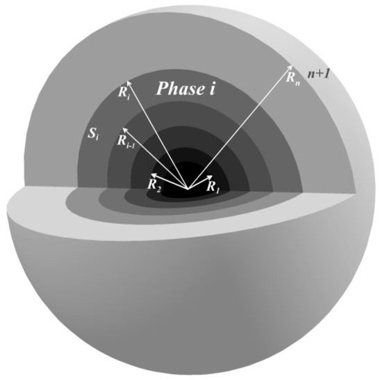
Figure 1.
The microstructure for n-layered isotropic spherical inclusion.
In Figure 1, indicates the phase number , is the sphere number , in the radius of the sphere . The model developed by Hervé et al. (1993) [31] enables the determination of effective elastic properties, namely, the compressibility modulus and the shear modulus , of a medium with phases by considering n-layered isotropic spherical inclusions. The model provides a solution for a medium defined by a spherical inclusion surrounded by layers, where each layer is considered as a phase (Figure 1).
Since the phase constituting the matrix is considered to extend to infinity, this model is regarded as a multi-scale homogenization model, and its solution allows for the estimation of macroscopic effective properties starting from a lower scale.
According to the model of Hervé and Zaoui (1993) [31], the effective bulk modulus and the shear modulus are given by Equations (1) and (2), respectively.
The bulk modulus is given by Equation (1).
The matrix is given in Appendix A by the expression (A4).
The effective shear modulus is obtained by solving the second order equation by the discriminant method through a Python program considering the coefficients , and detailed in Appendix A.
To address the question regarding the relevance of DH and MS methods, we have chosen to consider the solution of this model for a three-phase medium as the solution for the direct method and that of a two-phase medium as the solution used in two steps for the MS method.
3. Three-Phase Model
The medium of the three-phase model consists of three nested spheres. The first phase is an inclusion surrounded by the second phase, both nested within the third phase considered a matrix (Figure 2).
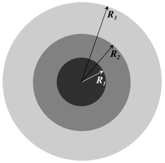
Figure 2.
Three-phase model illustration. is the inclusion radius (phase1), is the coating radius, and is the matrix radius.
So, the effective properties, bulk, and shear moduli are calculated in one step with Equations (3) and (4).
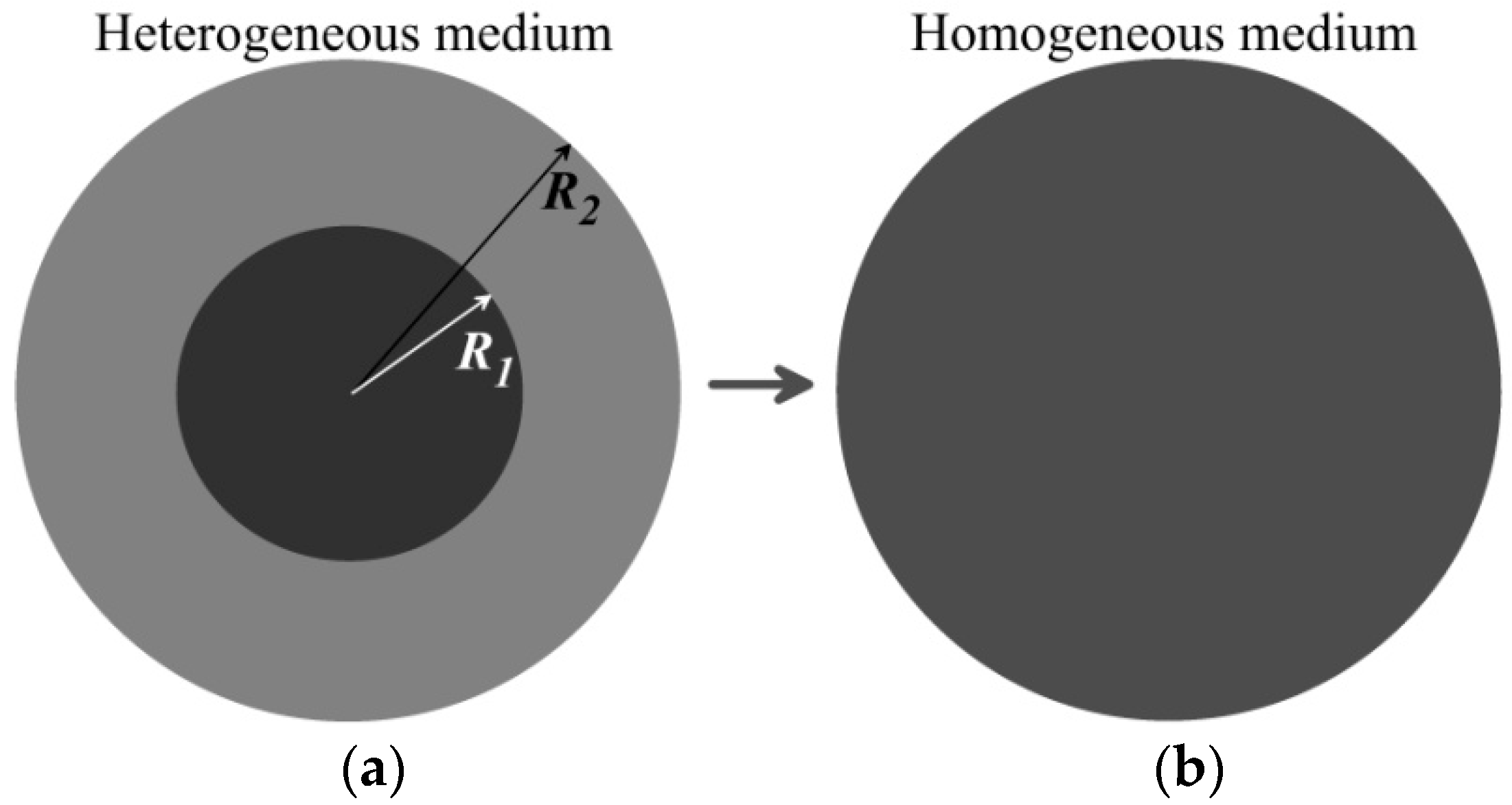
In this study, the solution of the model for phases, as illustrated in Figure 3, is referred to as the DH method because it allows for the estimation of effective properties in a single step.
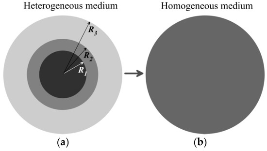
Figure 3.
Illustration of the direct homogenization method. (a) Three-phase medium. (b) Equivalent homogeneous medium.
4. Two-Phase Model
The medium of the two-phase model consists of two nested spheres: an inclusion nested within a matrix (Figure 4).

Figure 4.
Two-phase model illustration. is the inclusion radius, is the matrix radius. (a) Two-phase medium. (b) Equivalent homogeneous medium.
5. The Multistep Method
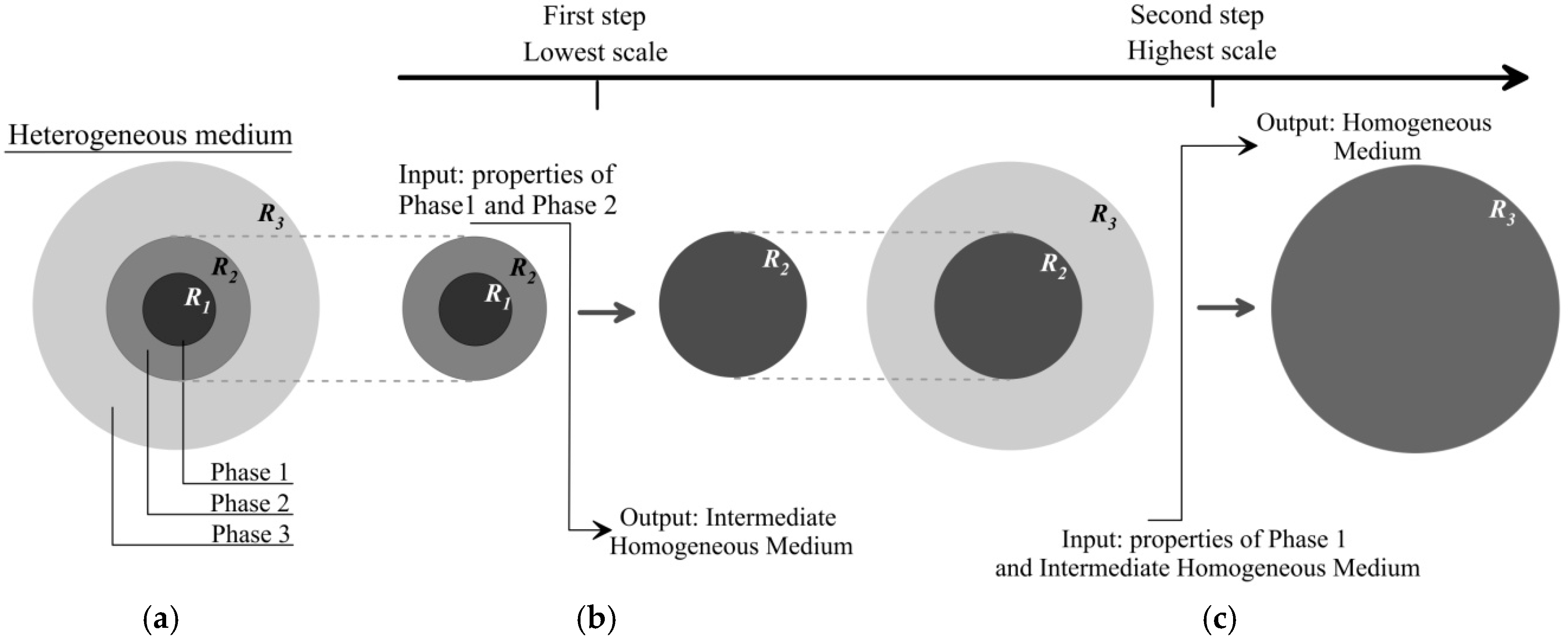
The MS method is a technique that is used to calculate an effective property of a heterogeneous media composed of a matrix and inclusions in many steps. This technique consists of calculating the homogenization of two phases and then using the obtained results to homogenize with the next phase. In the MS method, the effective properties, bulk, and shear moduli are calculated in two steps according to the number of phases as shown in Figure 5.
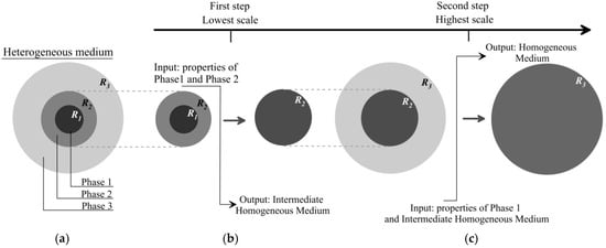
Figure 5.
Illustration of the two-step homogenization method for the 3-phase medium. (a) Three-phase medium. (b) First step of homogenization of phases 1 and 2. (c) Second step of homogenization.
In this technique, successive homogenizations are carried out from the lowest scale to the highest one to obtain the total effective property of a medium. It is also considered an MS method.
The MS method involves using the two-phase model to determine the effective properties of a three-phase medium, as shown in Figure 5a, in two steps.
The first step involves determining the effective properties, known as properties of the intermediate homogeneous medium (IHM), as shown in Figure 5a, for the two phases 1 and 2 using the solutions of Equations (5) and (6). The second step involves applying the same equations to the two IHM phases and the matrix (phase 3) to obtain the equivalent homogeneous medium of the three-phase medium, as depicted in Figure 5c.
6. Analytical Homogenization Study
In this section, the effective elastic properties, bulk, and shear moduli of the studied configuration are calculated, using the analytical homogenization model described in Section 2, by the two methods, ADH and AMS.
6.1. Limit of the Young’s Modulus Contrast Effect
The considered medium is composed of a multi-layered sphere that has three phases, 1, 2, and 3, where the radius of the matrix always equals 1. The Poisson ratio ν is equal to 0.3 in all the study models. It should be noted that before starting the calculations, a contrast check must be performed to determine its limit effect on the two properties, and . This is accomplished by taking and the contrasts and are expressed by
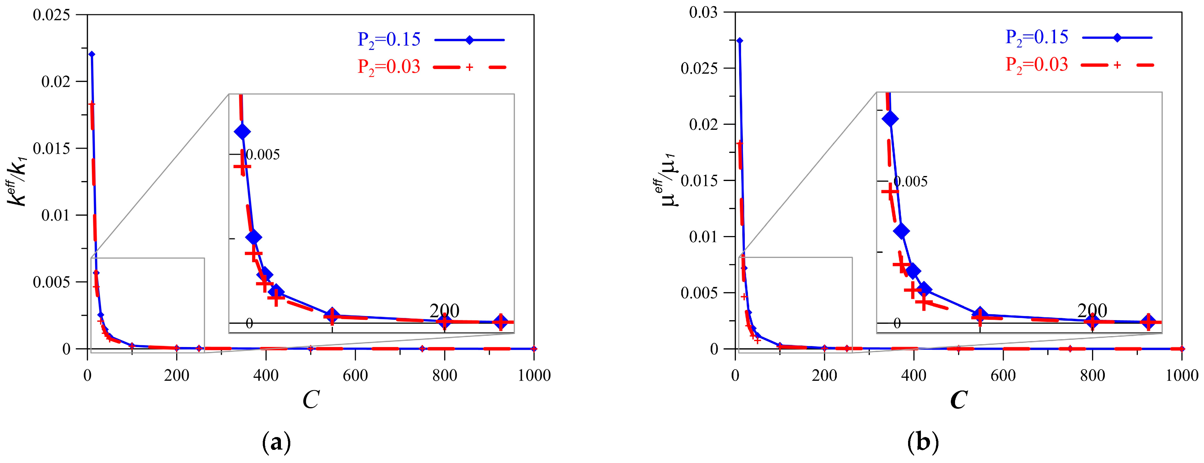
The limit effect of the contrast on the properties is represented in Figure 6. It is quite clear that this effect has stabilized at . Therefore, in this study, the variation of the contrast cannot exceed 200.
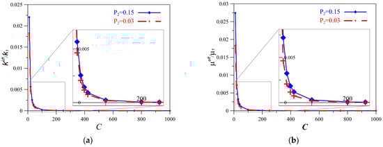
Figure 6.
The limit effect of the contrast on the effective properties the fraction of the first phase , the fraction of the second phase and , Poisson coefficient . (a) bulk modulus , (b) shear modulus .
6.2. Effective Elastic Properties versus the Volume Fractions of the Phases
The main objective of this part is to show the volume fraction effect on the effective bulk and shear moduli of the Hervé et al. (1993) model [31] for the two cases of phase numbers, and . The calculations are performed by varying the volume fraction of the first phase and the volume fraction of the second phase. The two homogenization methods, ADH and AMS, are used. The obtained results are then compared to evaluate the relevance of global and by-step homogenizations.
The results of the calculations are presented for three different volume fractions of phase 1, which are . Different contrasts are considered, , for each volume fraction of phase 1. The obtained results, for only the volume fraction , are displayed in Table A11 in Appendix C.
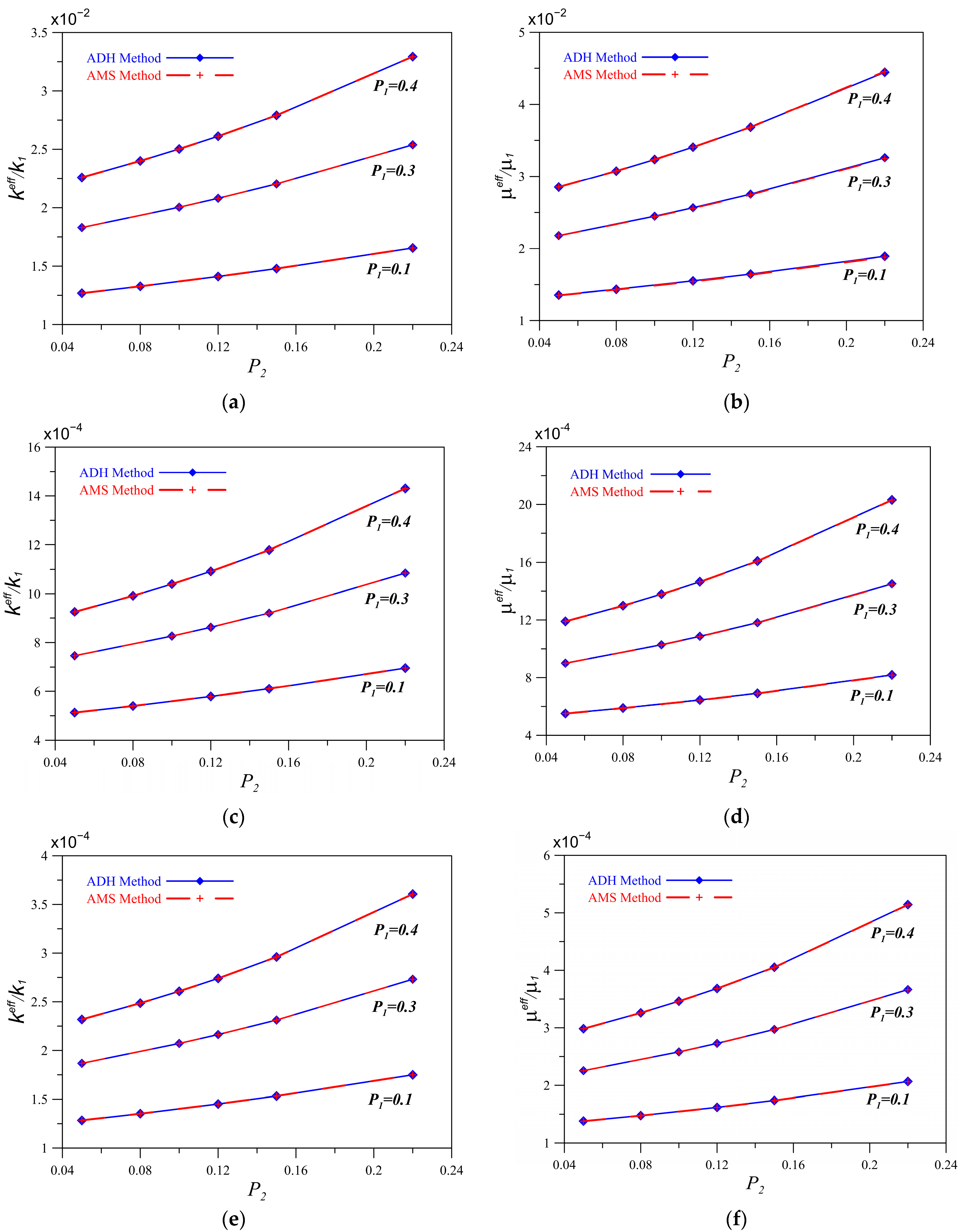
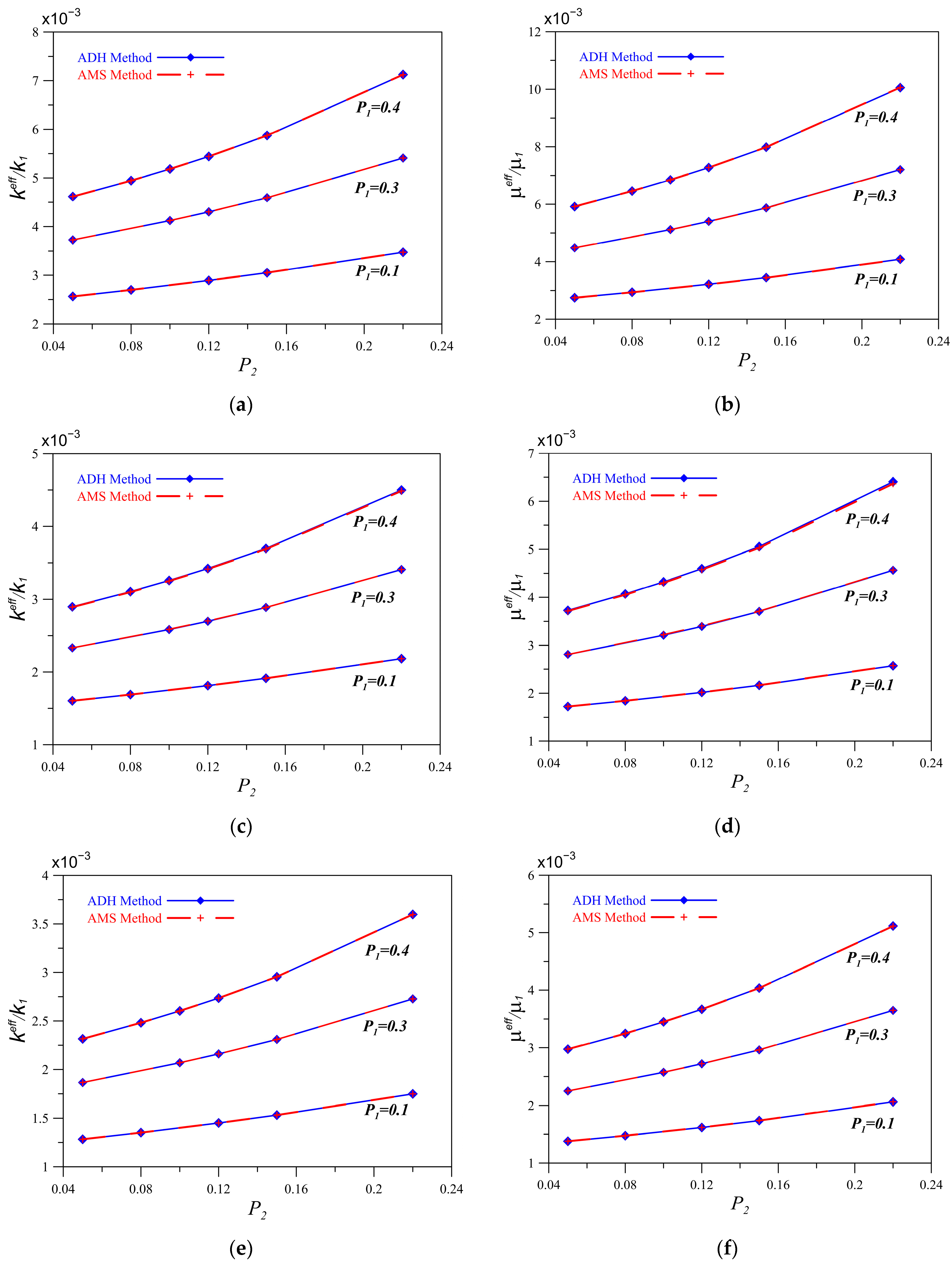
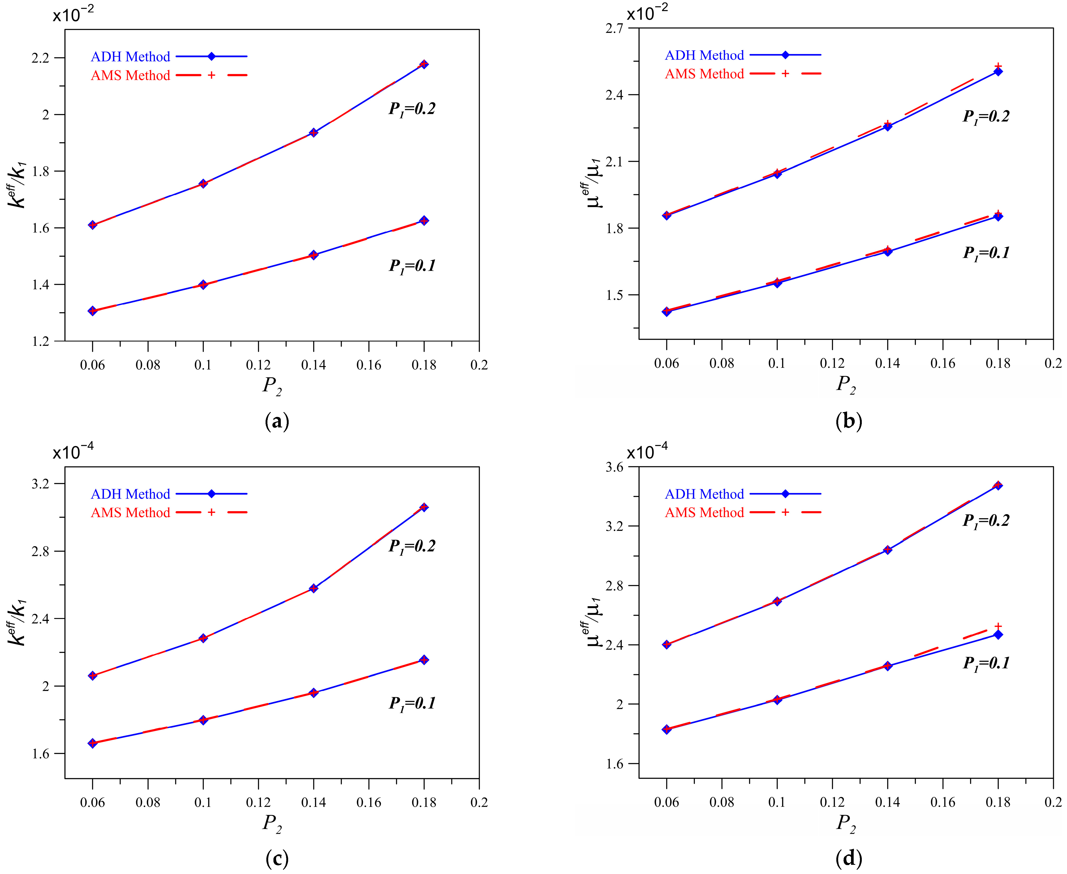
In Figure 7, the variation of the normalized effective properties as functions of the volume fractions of the second phase is illustrated.
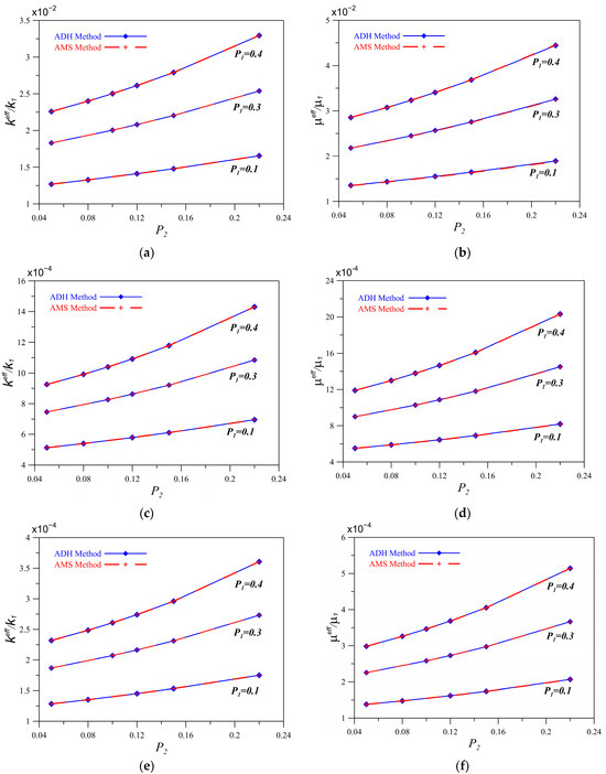
Figure 7.
Effective properties of bulk and shear moduli of the microstructure obtained with the two methods, ADH and AMS, for different volume fractions , (a,b) ; (c,d) ; (e,f) .
For a good comparison, the results obtained by the two methods, ADH and AMS, are superimposed.
The curves in Figure 7 exhibit the results, which are displayed in Table 1, of the effective normalized properties of bulk modulus and shear modulus calculated by the ADH and AMS methods. On the one hand, they show that the effective normalized properties and vary proportionally with the volume fraction of the interphase 2. On the other hand, the increase in the volume fraction of the inclusion 1 increases the effective elastic properties, but combined with the present variation of the contrast between the three phases, the contrast has the effect of decreasing the two effective elastic properties of the medium. This decrease becomes more important as the contrast increases (Figure 7e,f), i.e., when the inclusion 1 becomes more rigid than the matrix 3 of the medium.

Table 1.
The properties of the different phases with contrasts .
The results presented in Figure 7a–f show clearly that there is no difference between the obtained results by DH and MS methods, and the curves are perfectly confounded. From this part, it can be concluded that for the Hervé et al. (1993) model [31], which is composed of a multi-layered sphere, the obtained results of the effective elastic bulk and shear moduli are the same whether they are homogenized by the ADH and AMS methods.
6.3. Effective Elastic Properties versus the Contrasts of the Phases
This part is devoted to the study of the effect of the contrast variation of the medium phases on the effective elastic properties and . Unlike the previous Section 6.2 where the two contrasts and between the three phases, the inclusion 1, the interphase 2, and the matrix 3 were taken , in the present section, these two contrasts are considered different, . Three contrast variation series will be tested. The results of the normalized effective properties of the first contrast variation series, given in Table 2, are illustrated in Figure 8.
Table 2.
The properties of the different phases with contrasts .
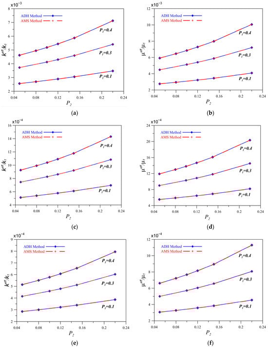
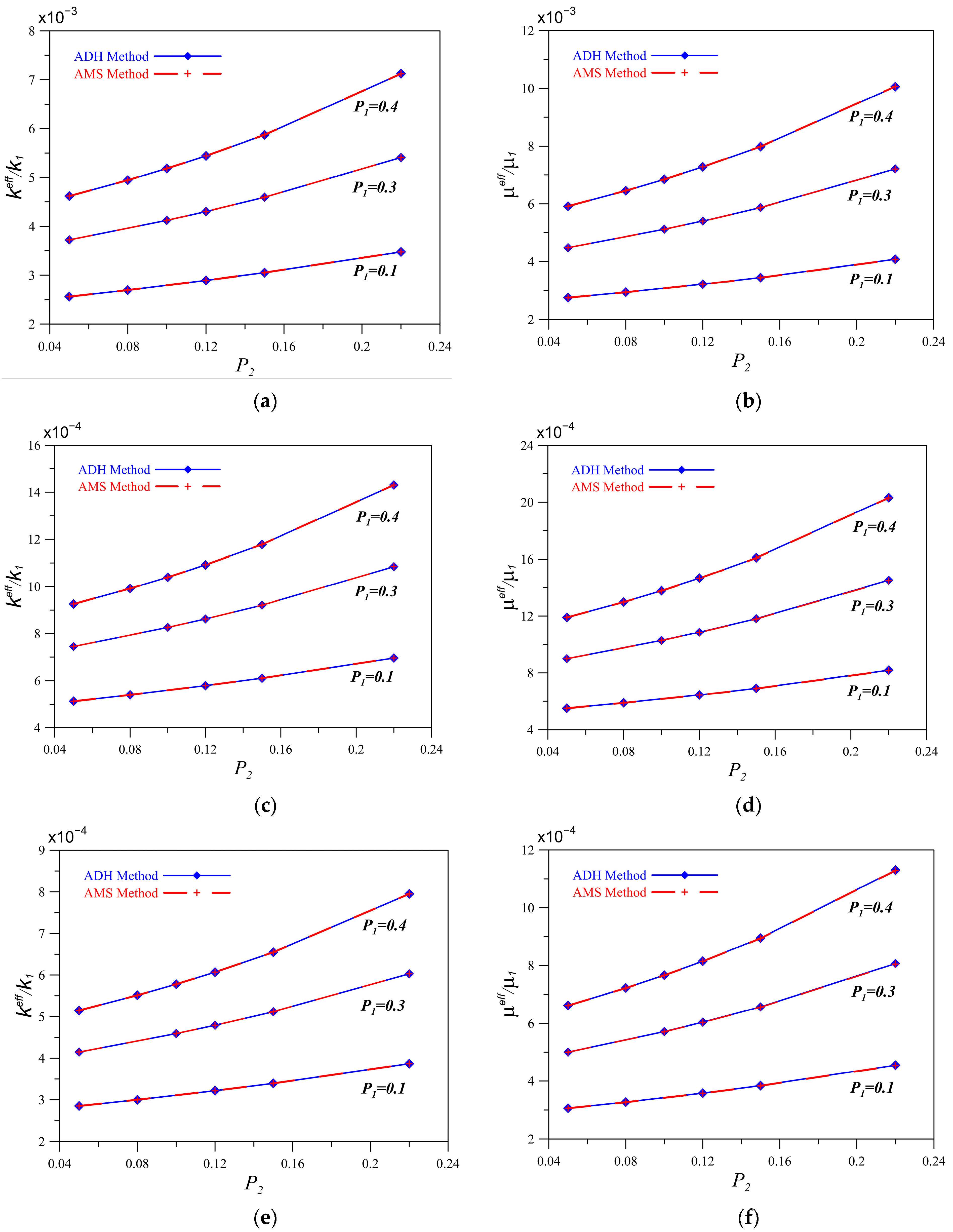
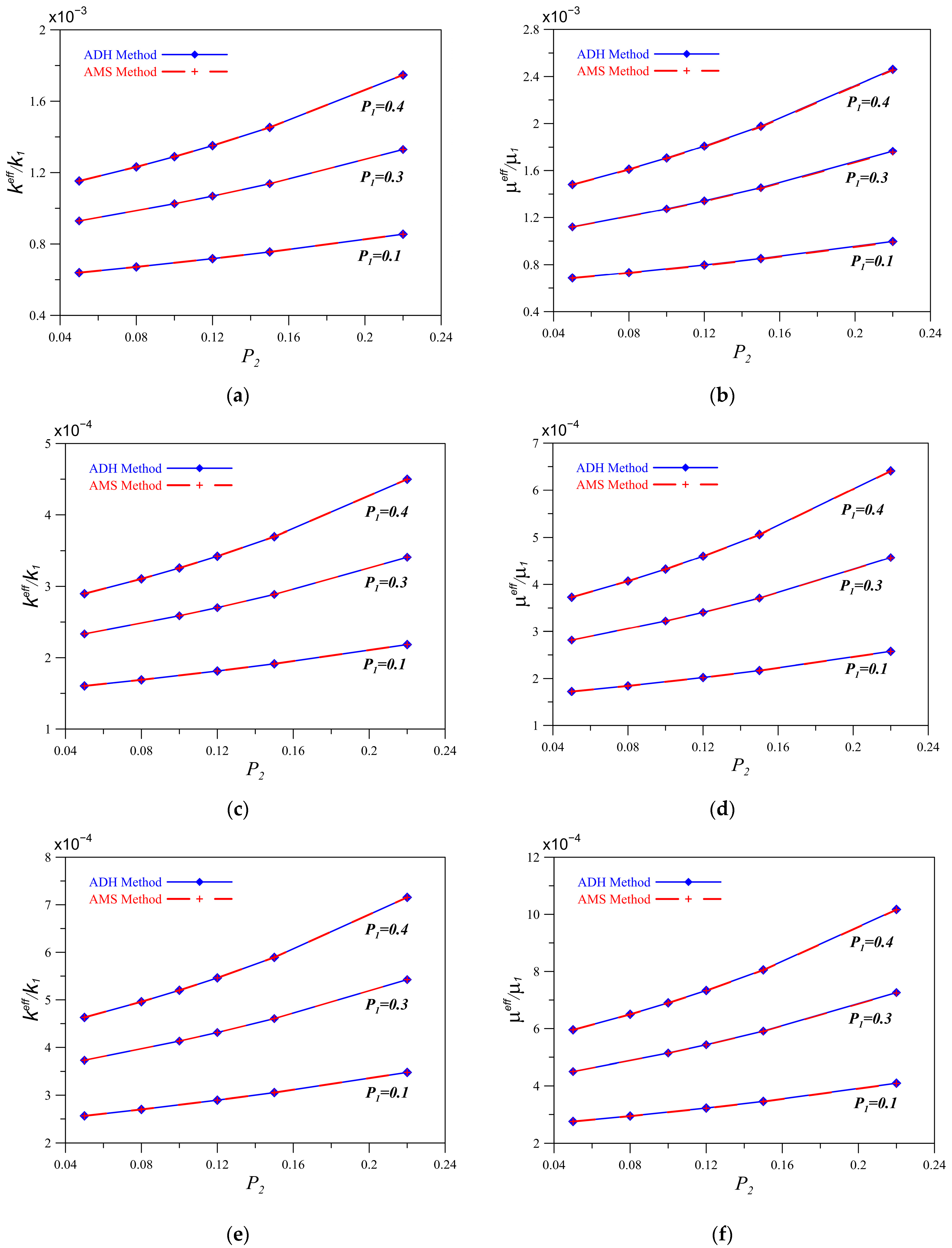
Figure 8.
Effective properties of bulk and shear moduli for the microstructure obtained with the two methods, ADH and AMS, for different volume fractions , , (a,b) ; (c,d) ; (e,f) .
The results of the normalized effective properties of the second contrast variation series, given in Table 3, are illustrated in Figure 9.
Table 3.
The properties of the different phases with contrasts ; .
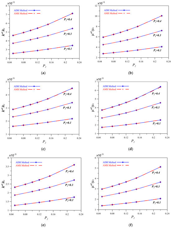
Figure 9.
Effective properties of bulk and shear moduli of the microstructure obtained with the two methods, ADH and AMS, for different volume fractions , , (a,b) ; (c,d) ; (e,f) .
The results of the normalized effective properties of the third contrast variation series, given in Table 4, are illustrated in Figure 10.
Table 4.
The properties of the different phases with contrasts ; .
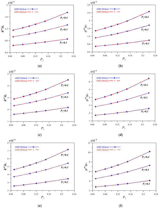
Figure 10.
Effective properties of bulk and shear moduli of the microstructure obtained by the two methods, ADH and AMS, for different volume fractions , , (a,b) ; (c,d) ; (e,f) .
The variations of the normalized effective elastic properties of bulk and shear moduli of the model used by Hervé et al. (1993) [31] as functions of the interphase volume fraction , obtained for the present considered case where the contrasts between the three phases are different ) are shown by the curves in Figure 8, Figure 9 and Figure 10. It must be remembered that for each one of Figure 8, Figure 9 and Figure 10, the variation has been represented for three values of the volume fraction of the inclusion 1, and for each of these values, two curves are represented: one corresponds to the effective property calculated by the ADH method and the other corresponds to that calculated by the AMS method, as indicated in the legend of the figures. These two curves are superimposed because the values of the homogenized properties are the same. The interpretation of the results obtained in the present section is quasi-identical to that of Section 6.2. For all the three contrast variation series, the normalized effective elastic properties present a variation that is proportional to the volume fraction of the interphase 2. The combined variation of the volume fraction of the inclusion 1 and the variation of the contrasts and , between Young’s moduli of the inclusion 1, the interphase 2, and the matrix 3 of the medium, has shown that when increases, regardless of and , the effective elastic properties increase, and when the contrasts increase, the effective elastic properties decrease. Note that the numerical results of the two methods compared with the second-order bounds of HS, for the volume fraction and different contrasts, are presented in Table A1, Table A2, Table A3, Table A4, Table A5, Table A6, Table A7, Table A8, Table A9, Table A10 and Table A11 given in Appendix C. The expressions of the HS bounds are given in Appendix B.
A detailed comparison, based on superimposing obtained results, of the effect of the different contrast variation series on the effective elastic properties is illustrated by the curves in Figure 11. The most important result obtained from this section is that whatever the combinations between all the considered parameters, the volume fraction , the contrasts , and regardless of the calculation method used—ADH or AMS—the homogenized elastic bulk and shear moduli of the Hervé et al. (1993) model [31] are identical since the error does not reach 1% for all the cases of the present study, as shown in Table A1, Table A2, Table A3, Table A4, Table A5, Table A6, Table A7, Table A8, Table A9, Table A10 and Table A11 in Appendix C.
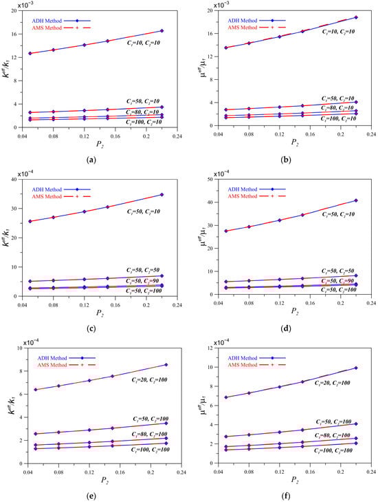
Figure 11.
Effective properties of bulk modulus (a,c,e) and shear modulus (b,d,f) of the microstructure obtained with the two methods, ADH and AMS, for different volume fractions , (a,b) ), (, )(, ), (); (c,d) )(, )(, ), (); (e,f) ), (, )(, ), ().
7. Numerical Homogenization Study
This section aims to verify the same principle mentioned in the first part of this study by a numerical homogenization based on the finite element calculation using the two methods NDH and NMS.
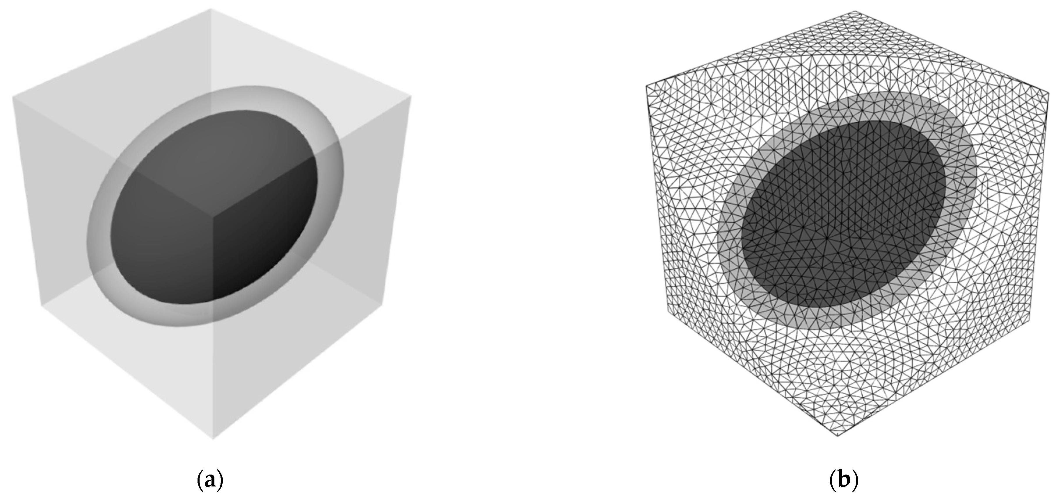
Unlike the first analytical part, two configurations are considered. The first one is similar to the model described in Section 2, involving spherical shapes. This form was adopted by the model’s authors for purely mathematical reasons. To highlight the effect of a shape, a second form is considered in this section. For this purpose, the ellipsoidal shape was chosen as it is regarded in all cases as the most different shape from the spherical form. To ensure that the second configuration is entirely different from the first, a cubic matrix was considered.
7.1. Materials and Method
For the spherical configuration, the two volume fractions and are considered. In contrast, for the ellipsoidal configuration, the volume fraction is limited to and . This limitation to a maximum volume fraction of is due to the shape of the ellipsoid, which does not allow for exceeding this fraction without the coated inclusion overlapping with the matrix.
For a more general study, several contrasts and , defining the different phase’s materials are treated.
In the case of numerical homogenization, specific boundary conditions are imposed. In this study, the boundary condition “Kinematic Uniform Boundary Conditions (KUBC)” is used for the determination of the effective bulk modulus and the effective shear modulus for the two considered configurations.
This condition consists of imposing a displacement on the contour such that:
with D a symmetrical second-rank tensor of imposed macroscopic strains, such as:
The effective bulk modulus and the effective shear modulus are defined by Equations (10) and (11), respectively
With
The symbol designates the average value.
To mesh the different microstructures studied, a free mesh is used with an average of 50,000 quadratic 10-node finite elements as shown in Figure 12 and Figure 13.
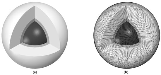
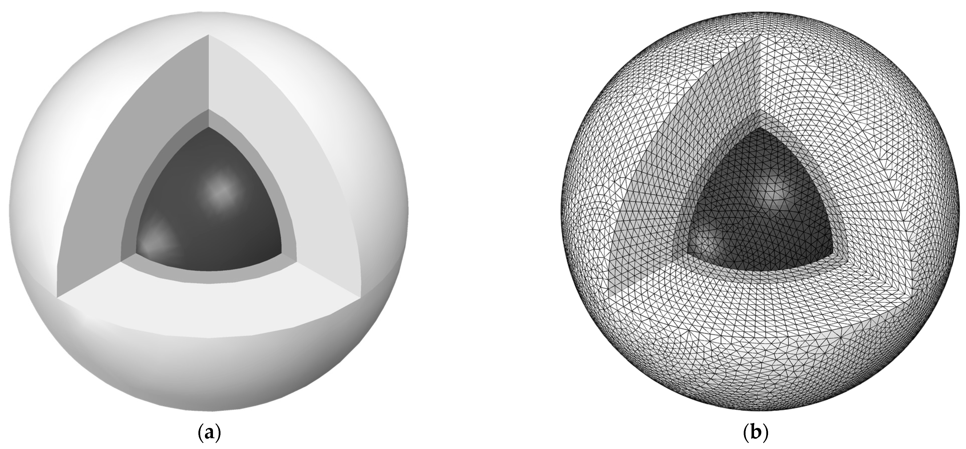
Figure 12.
Meshed microstructure illustration of the first configuration: (a) initial microstructure, (b) meshed microstructure.
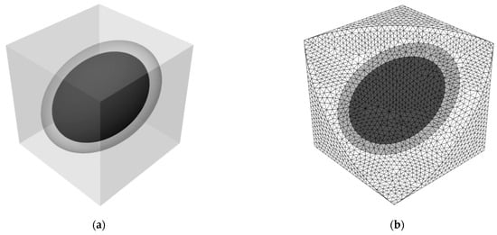
Figure 13.
Meshed microstructure illustration of the second configuration: (a) initial microstructure, (b) meshed microstructure.
7.2. Results and Discussion
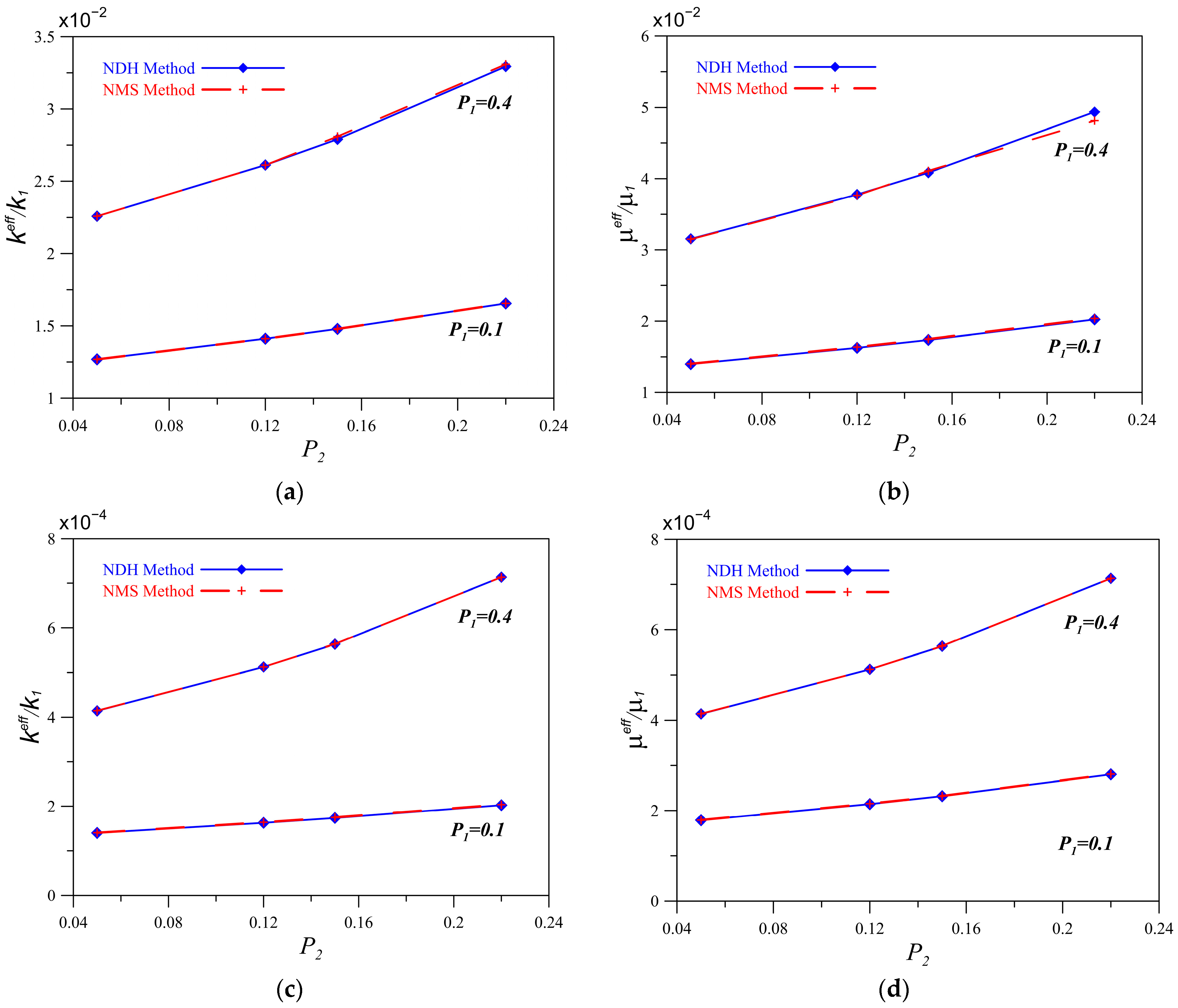
All numerical results of the elastic properties, bulk, and shear moduli of the first studied configuration, using the two methods, NDH and NMS, are presented in Figure 14. The normalized properties increase significantly for the volume fraction but slightly for the volume fraction .
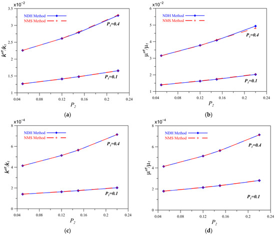
Figure 14.
Effective properties of bulk modulus (a,c) and shear modulus (b,d) of the first configuration obtained by the two methods, NDH and NMS, using the numerical homogenization for different volume fractions , (a,b) ; (c,d) .
For the first configuration, the comparison of numerical results obtained by the NDH method and the NMS method clearly shows that both methods provide estimates of the effective properties with the same precision. Note that the error is less than 1% (see Table A12 and Table A13 in Appendix C). This implies that in the case of numerical homogenization, both the NDH method and the NMS method similarly ensure the effective properties of multi-phase heterogeneous media.
An example of additional results of a deformed studied composite due to the two boundary conditions, bulk and shear, are presented in Figure 15 with the stress iso-values represented by the color variation in Figure 15c. The stress distribution indicates that the bluer the color, the lower the stress value and the redder the color, the higher the stress value.
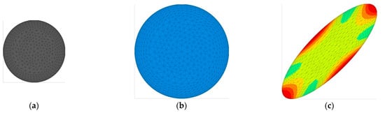
Figure 15.
Deformed microstructure illustration: (a) initial microstructure, (b) bulk, (c) shear.
All numerical results of the elastic properties, bulk, and shear moduli of the second configuration, using the NDH and NMS methods are presented in Figure 16.
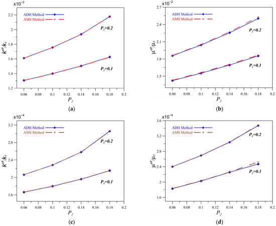
Figure 16.
Effective properties of bulk modulus (a,c) and shear modulus (b,d) of the second configuration obtained by the two methods, NDH and NMS, using the numerical homogenization for different volume fractions , (a,b) ; (c,d) .
For the second configuration, as shown in Table A14 and Table A15 in Appendix C, the comparison of numerical results obtained using the NDH method and the NMS method clearly demonstrates that both methods estimate the effective properties with the same precision, with a maximum error of less than 3%. These results indicate that even for configurations completely different from those of the model, both the NDH method and the NMS method similarly ensure accurate effective properties of multi-phase heterogeneous media.
8. Conclusions
The main purpose of this study is to compare the relevance of two hypotheses of multi-scale homogenization. On the one hand, direct homogenization (DH), based on a single representation at a level that can contain all the heterogeneities of a medium, is supposed to be sufficient to determine the effective properties of this medium. On the other hand, the results obtained by the DH method do not guarantee a good estimation, and the effective properties of a heterogeneous medium must be determined by successive MS homogenizations from the lowest to the highest level.
Two different studies have been carried out. The first is analytical homogenization and the second is numerical finite element homogenization.
The analytical homogenization has been achieved by considering the multi-layered sphere model of Hervé et al. (1993) model [31].
Numerical homogenization was conducted by considering two distinct configurations. The first configuration matches the analytical model, represented by spherical shapes. The second configuration is entirely different from the first, featuring an ellipsoidal inclusion drowned in a cubic matrix.
All configurations have been developed to estimate the effective elastic properties, bulk modulus, and shear modulus of multi-phase heterogeneous media. The three-phase model has been chosen as the solution for the DH method, and the two-phase as the solution used in the two-step MS method.
The calculations have been conducted by studying the effect of the parameters, which are the volume fractions of the different phases of the medium and the property contrasts between different phases. The effective elastic bulk modulus and shear modulus have been determined as functions of the second phase, considered as the interphase, of the medium. The obtained results show that the effective properties vary proportionally with the considered volume fraction for all the several cases tested, regardless of the variation of the other volume fractions or the different contrasts. The effect of the volume fraction of the first phase, considered as the inclusion of the medium, has been tested, and the obtained results indicate that the effective elastic properties increase with the increase of this volume fraction. Several contrast variation series have been considered, from assuming the contrasts between the first and the second phase and the second and the third phase to be equal to assuming these two contrasts to be different. From all these contrast variations, combined with the variation of the different volume fractions, many results have emerged, and the most important is that the effective elastic bulk and shear moduli decrease when the contrasts increase and that the two methods gave the same results of the elastic properties of the studied model.
The main conclusion that can be deducted from this study is that both methods of homogenization—DH and MS methods—are efficient for the two studies, analytical and numerical homogenizations since they ensure the same effective elastic properties of a heterogeneous medium with the same precision. Therefore, the application of the direct method is recommended compared with the step-by-step method because it requires less calculation and calculation time, especially when the heterogeneous medium contains a significant number of heterogeneities.
Author Contributions
Methodology, N.K., M.M., T.K., W.K. and Y.D.; Software, N.K., M.M., T.K., O.O. and Y.D.; Validation, T.K., W.K., M.M., N.K. and Y.D.; Formal analysis, N.K., M.M., T.K., W.K. and Y.D.; Resources, M.M., W.K., N.K. and T.K.; Data curation, N.K., W.K., M.M. and Y.D.; Writing—original draft, M.M., N.K. and W.K.; Visualization, T.K., M.M, W.K. and N.K.; Supervision, M.M., T.K. and W.K.; Project administration, M.M., T.K. and W.K.; Funding acquisition, T.K. and W.K. All authors have read and agreed to the published version of the manuscript.
Funding
This research received no external funding.
Informed Consent Statement
Not applicable.
Data Availability Statement
The original contributions presented in the study are included in the article, further inquiries can be directed to the corresponding author.
Conflicts of Interest
The authors declare no conflict of interest.
Nomenclature
| the sphere number i | r | Polar coordinate | |
| the phase number | Radius of phase | ||
| Bulk modulus of phase n | C | Contrast between phases | |
| Shear modulus of phase n | Volume fraction of phase | ||
| Radius of sphere n | E | Young modulus | |
| Calculated matrix element | Poisson’s ratio of the phase n |
Appendix A
In the following, we present the formulation details of the Hervé et al. (1993) model [31]:
The coefficients , and in the Equations (A2), (A4) and (A6) are expressed by:
is a tensor expressed by:
The two conditions that result from the continuity of and at the interface between phases and may be written in the form:
where and is the expressed by (A7):
The system of two simultaneous Equation (A6) is solved for and
By substituting, Equation (A7) becomes:
Therefore, one gets:
Appendix B
In this appendix, the Hashin and Shtrikman second-order bounds for n-phase materials are presented.
The Hashin and Shtrikman [33] bounds of bulk modulus are given by Equations (A12) and (A13) as:
where , , and are expressed by Equations (A14)–(A17) respectively, as:
with , volume fraction of phase in R3. This way one can bound the homogenized bulk modulus :
Let us now consider the Hashin and Shtrikman [33] bounds of shear modulus :
The lower bound is expressed by Equation (A19),
And the highest bound is expressed by Equation (A20), as
with the parameters , , and are defined by the expressions (A21)–(A24), respectively.
The effective property is always surrounded by the two bounds, such that:
In the case of two-phase composites, the bounds expressions of the bulk modulus k are expressed by Equations (A26) and (A27) and for by Equations (A28) and (A29) for the shear modulus:
Appendix C
In this appendix, the numerical results of the two methods compared with the second-order bounds of HS, for the volume fraction and different contrasts, are presented.
Table A1.
The two methods, DH and MS, normalized effective properties comparison for different volume fractions and the contrast . The values of the normalized properties must be multiplied by .
Table A1.
The two methods, DH and MS, normalized effective properties comparison for different volume fractions and the contrast . The values of the normalized properties must be multiplied by .
| Lower Bond HS− | DH Method | MS Method | Upper Bond HS+ | Errors % | ||||||
|---|---|---|---|---|---|---|---|---|---|---|
| Errk | Errµ | |||||||||
| 0.05 | 1.2646 | 1.3375 | 1.2680 | 1.3525 | 1.2680 | 1.3556 | 5.5324 | 6.9520 | 0 | 0.2306 |
| 0.08 | 1.3220 | 1.4083 | 1.3271 | 1.4307 | 1.3271 | 1.4362 | 5.8050 | 7.2299 | 0 | 0.3816 |
| 0.12 | 1.4041 | 1.5094 | 1.4111 | 1.5436 | 1.4111 | 1.5519 | 6.1720 | 7.6025 | 0 | 0.5388 |
| 0.15 | 1.4705 | 1.5907 | 1.4788 | 1.6359 | 1.4788 | 1.6457 | 6.4498 | 7.8835 | 0 | 0.5980 |
| 0.22 | 1.6436 | 1.8017 | 1.6552 | 1.8806 | 1.6552 | 1.8919 | 7.1070 | 8.5444 | 0 | 0.5976 |
Table A2.
The two methods, DH and MS, normalized effective properties comparison for different volume fractions and the contrasts . The values of the normalized properties must be multiplied by .
Table A2.
The two methods, DH and MS, normalized effective properties comparison for different volume fractions and the contrasts . The values of the normalized properties must be multiplied by .
| Lower Bond HS− | DH Method | MS Method | Upper Bond HS+ | Errors % | ||||||
|---|---|---|---|---|---|---|---|---|---|---|
| Errk | Errµ | |||||||||
| 0.05 | 5.1252 | 5.4575 | 5.1293 | 5.5073 | 5.1293 | 5.5113 | 420.9916 | 564.5936 | 0 | 0.0723 |
| 0.08 | 5.3931 | 5.8019 | 5.3991 | 5.8829 | 5.3991 | 5.8900 | 427.4945 | 570.9778 | 0 | 0.1202 |
| 0.12 | 5.7811 | 6.3004 | 5.7895 | 6.4376 | 5.7895 | 6.4491 | 436.1852 | 579.5011 | 0 | 0.1778 |
| 0.15 | 6.0982 | 6.7074 | 6.1084 | 6.9008 | 6.1084 | 6.9148 | 442.7183 | 585.9018 | 0 | 0.2039 |
| 0.22 | 6.9424 | 7.7893 | 6.9571 | 8.1697 | 6.9571 | 8.1876 | 458.0126 | 600.8643 | 0 | 0.2194 |
Table A3.
The two method’s, DH and MS, normalized effective properties comparison for different volumes fractions and the contrasts . The values of the normalized properties must be multiplied by .
Table A3.
The two method’s, DH and MS, normalized effective properties comparison for different volumes fractions and the contrasts . The values of the normalized properties must be multiplied by .
| Lower Bond HS− | DH Method | MS Method | Upper Bond HS+ | Errors % | ||||||
|---|---|---|---|---|---|---|---|---|---|---|
| Errk | Errµ | |||||||||
| 0.05 | 1.2831 | 1.3675 | 1.2837 | 1.3793 | 1.2847 | 1.3808 | 412.6545 | 556.4034 | 0.0007 | 0.1131 |
| 0.08 | 1.3514 | 1.4557 | 1.3522 | 1.4749 | 1.3522 | 1.4760 | 415.9832 | 559.6525 | 0 | 0.0705 |
| 0.12 | 1.4504 | 1.5836 | 1.4515 | 1.6173 | 1.4515 | 1.6188 | 420.4268 | 563.9875 | 0 | 0.0948 |
| 0.15 | 1.5314 | 1.6883 | 1.5327 | 1.7363 | 1.5328 | 1.7382 | 423.7634 | 567.2409 | 0 | 0.1078 |
| 0.22 | 1.7477 | 1.9675 | 1.7497 | 2.0638 | 1.7497 | 2.0663 | 431.5621 | 574.8394 | 0 | 0.1180 |
Table A4.
The two methods, DH and MS, normalized effective properties comparison for different volume fractions and the contrasts , . The values of the normalized properties must be multiplied by .
Table A4.
The two methods, DH and MS, normalized effective properties comparison for different volume fractions and the contrasts , . The values of the normalized properties must be multiplied by .
| Lower Bond HS− | DH Method | MS Method | Upper Bond HS+ | Errors % | ||||||
|---|---|---|---|---|---|---|---|---|---|---|
| Errk | Errµ | |||||||||
| 0.05 | 1.2811 | 1.3640 | 1.2820 | 1.3763 | 1.2820 | 1.3771 | 44.2205 | 58.5837 | 0 | 0.0646 |
| 0.08 | 1.3480 | 1.4500 | 1.3494 | 1.4700 | 1.3494 | 1.4716 | 45.7836 | 60.1442 | 0 | 0.1131 |
| 0.12 | 1.4450 | 1.5746 | 1.4515 | 1.6173 | 1.4469 | 1.6111 | 47.8793 | 62.2315 | 0.0031 | 0.3782 |
| 0.15 | 1.5242 | 1.6763 | 1.5266 | 1.7242 | 1.5266 | 1.7274 | 49.4598 | 63.8019 | 0 | 0.1813 |
| 0.22 | 1.7352 | 1.9467 | 1.7386 | 2.0411 | 1.7386 | 2.0450 | 53.1772 | 67.4826 | 0 | 0.1920 |
Table A5.
The two methods, DH and MS, normalized effective properties comparison for different volume fractions and the contrasts , . The values of the normalized properties must be multiplied by .
Table A5.
The two methods, DH and MS, normalized effective properties comparison for different volume fractions and the contrasts , . The values of the normalized properties must be multiplied by .
| Lower Bond HS− | DH Method | MS Method | Upper Bond HS+ | Errors % | ||||||
|---|---|---|---|---|---|---|---|---|---|---|
| Errk | Errµ | |||||||||
| 0.05 | 2.8475 | 3.0322 | 2.8498 | 3.0602 | 2.8497 | 3.0623 | 414.4485 | 558.1515 | 0 | 0.0689 |
| 0.08 | 2.9963 | 3.2235 | 2.9997 | 3.2686 | 2.9997 | 3.2728 | 418.1047 | 561.7224 | 0 | 0.1290 |
| 0.12 | 3.2119 | 3.5005 | 3.2166 | 3.5770 | 3.2166 | 3.5835 | 422.9860 | 566.4870 | 0 | 0.1837 |
| 0.15 | 3.3881 | 3.7266 | 3.3938 | 3.8344 | 3.3938 | 3.8424 | 426.6517 | 570.0631 | 0 | 0.2103 |
| 0.22 | 3.8571 | 4.3277 | 3.8654 | 4.5396 | 3.8654 | 4.5499 | 435.2209 | 578.4158 | 0 | 0.2277 |
Table A6.
The two methods, DH and MS, normalized effective properties comparison for different volume fractions and the contrasts , . The values of the normalized properties must be multiplied by .
Table A6.
The two methods, DH and MS, normalized effective properties comparison for different volume fractions and the contrasts , . The values of the normalized properties must be multiplied by .
| Lower Bond HS− | DH Method | MS Method | Upper Bond HS+ | Errors % | ||||||
|---|---|---|---|---|---|---|---|---|---|---|
| Errk | Errµ | |||||||||
| 0.05 | 2.5614 | 2.7268 | 2.5631 | 2.7508 | 2.5631 | 2.7523 | 47.4935 | 61.9657 | 0 | 0.0547 |
| 0.08 | 2.6953 | 2.8988 | 2.6978 | 2.9379 | 2.6978 | 2.9407 | 50.4314 | 64.9752 | 0 | 0.09391 |
| 0.12 | 2.8892 | 3.1479 | 2.8926 | 3.2146 | 2.8926 | 3.2189 | 54.3894 | 69.0121 | 0 | 0.1325 |
| 0.15 | 3.0476 | 3.3512 | 3.0518 | 3.4456 | 3.0518 | 3.4507 | 57.3889 | 72.0583 | 0 | 0.1495 |
| 0.22 | 3.4694 | 3.8917 | 3.4754 | 4.0780 | 3.4754 | 4.0842 | 64.4933 | 79.2281 | 0 | 0.1526 |
Table A7.
The two methods, DH and MS, normalized effective properties comparison for different volume fractions and the contrasts , . The values of the normalized properties must be multiplied by .
Table A7.
The two methods, DH and MS, normalized effective properties comparison for different volume fractions and the contrasts , . The values of the normalized properties must be multiplied by .
| Lower Bond HS− | DH Method | MS Method | Upper Bond HS+ | Errors % | ||||||
|---|---|---|---|---|---|---|---|---|---|---|
| Errk | Errµ | |||||||||
| 0.05 | 1.6029 | 1.7075 | 1.6036 | 1.7221 | 1.6036 | 1.7226 | 46.7585 | 61.2569 | 0 | 0.0345 |
| 0.08 | 1.6877 | 1.8171 | 1.6887 | 1.8410 | 1.6887 | 1.8421 | 49.7160 | 64.2878 | 0 | 0.0596 |
| 0.12 | 1.8108 | 1.9759 | 1.8122 | 2.0173 | 1.8122 | 2.0190 | 53.7008 | 68.3538 | 0 | 0.0845 |
| 0.15 | 1.9115 | 2.1057 | 1.9132 | 2.1648 | 1.9132 | 2.1669 | 56.7208 | 71.4220 | 0 | 0.0955 |
| 0.22 | 2.1801 | 2.4517 | 2.1825 | 2.5701 | 2.1825 | 2.5726 | 63.8747 | 78.6441 | 0 | 0.0977 |
Table A8.
The two methods, DH and MS, normalized effective properties comparison for different volume fractions and the contrasts , . The values of the normalized properties must be multiplied by .
Table A8.
The two methods, DH and MS, normalized effective properties comparison for different volume fractions and the contrasts , . The values of the normalized properties must be multiplied by .
| Lower Bond HS− | DH Method | MS Method | Upper Bond HS+ | Errors % | ||||||
|---|---|---|---|---|---|---|---|---|---|---|
| Errk | Errµ | |||||||||
| 0.05 | 1.2828 | 1.3669 | 1.2833 | 1.3784 | 1.2833 | 1.3788 | 46.5135 | 61.0206 | 0 | 0.0278 |
| 0.08 | 1.3510 | 1.4551 | 1.3517 | 1.4741 | 1.3517 | 1.4748 | 49.4776 | 64.0587 | 0 | 0.0480 |
| 0.12 | 1.4500 | 1.5830 | 1.4509 | 1.6161 | 1.4509 | 1.6172 | 53.4712 | 68.1343 | 0 | 0.0680 |
| 0.15 | 1.5310 | 1.6876 | 1.5321 | 1.7349 | 1.5321 | 1.7362 | 56.4980 | 71.2098 | 0 | 0.0769 |
| 0.22 | 1.7472 | 1.9666 | 1.7488 | 2.0619 | 1.7488 | 2.0635 | 63.6684 | 78.4493 | 0 | 0.0788 |
Table A9.
The two methods, DH and MS, normalized effective properties comparison for different volume fractions and the contrasts , . The values of the normalized properties must be multiplied by .
Table A9.
The two methods, DH and MS, normalized effective properties comparison for different volume fractions and the contrasts , . The values of the normalized properties must be multiplied by .
| Lower Bond HS− | DH Method | MS Method | Upper Bond HS+ | Errors % | ||||||
|---|---|---|---|---|---|---|---|---|---|---|
| Errk | Errµ | |||||||||
| 0.05 | 0.6697 | 0.6779 | 0.6852 | 0.6852 | 0.6392 | 0.6865 | 41.6524 | 56.0155 | 0 | 0.1862 |
| 0.08 | 0.7153 | 0.7180 | 0.6714 | 0.7293 | 0.6714 | 0.7315 | 41.9719 | 56.3273 | 0 | 0.3077 |
| 0.12 | 0.7524 | 0.7756 | 0.7178 | 0.7938 | 0.7178 | 0.7973 | 42.3985 | 56.7434 | 0 | 0.4308 |
| 0.15 | 0.8505 | 0.8224 | 0.7554 | 0.8473 | 0.7554 | 0.8514 | 42.7189 | 57.0557 | 0 | 0.4890 |
| 0.22 | 0.6697 | 0.9457 | 0.8548 | 0.9918 | 0.8548 | 0.9970 | 43.4675 | 57.7850 | 0 | 0.5234 |
Table A10.
The two methods, DH and MS, normalized effective properties comparison for different volume fractions and the contrasts , . The values of the normalized properties must be multiplied by .
Table A10.
The two methods, DH and MS, normalized effective properties comparison for different volume fractions and the contrasts , . The values of the normalized properties must be multiplied by .
| Lower Bond HS− | DH Method | MS Method | Upper Bond HS+ | Errors % | ||||||
|---|---|---|---|---|---|---|---|---|---|---|
| Errk | Errµ | |||||||||
| 0.05 | 1.6034 | 1.7084 | 1.6042 | 1.7233 | 1.6042 | 1.7242 | 412.8962 | 556.6379 | 0 | 0.0488 |
| 0.08 | 1.6883 | 1.8180 | 1.6895 | 1.8425 | 1.6895 | 1.8440 | 416.2167 | 559.8789 | 0 | 0.0821 |
| 0.12 | 1.8114 | 1.9769 | 1.8131 | 2.0192 | 1.8131 | 2.0216 | 420.6492 | 564.2030 | 0 | 0.1172 |
| 0.15 | 1.9121 | 2.1068 | 1.9142 | 2.1670 | 1.9142 | 2.1699 | 423.9775 | 567.4483 | 0 | 0.1346 |
| 0.22 | 2.1809 | 2.4530 | 2.1839 | 2.5732 | 2.1839 | 2.5769 | 431.7566 | 575.0276 | 0 | 0.1463 |
Table A11.
The two methods, DH and MS, normalized effective properties comparison for different volume fractions and the contrasts , . The values of the normalized properties must be multiplied by .
Table A11.
The two methods, DH and MS, normalized effective properties comparison for different volume fractions and the contrasts , . The values of the normalized properties must be multiplied by .
| Lower Bond HS− | DH Method | MS Method | Upper Bond HS+ | Errors % | ||||||
|---|---|---|---|---|---|---|---|---|---|---|
| Errk | Errµ | |||||||||
| 0.05 | 2.5627 | 2.7290 | 2.5648 | 2.7540 | 2.5648 | 2.7561 | 413.6218 | 557.3413 | 0 | 0.0773 |
| 0.08 | 2.6967 | 2.9012 | 2.6997 | 2.9418 | 2.6997 | 2.9456 | 416.9174 | 560.5579 | 0 | 0.1297 |
| 0.12 | 2.8907 | 3.1504 | 2.8950 | 3.2193 | 2.8950 | 3.2253 | 421.3166 | 564.8494 | 0 | 0.1844 |
| 0.15 | 3.0493 | 3.3540 | 3.0545 | 3.4510 | 3.0545 | 3.4583 | 424.6198 | 568.0701 | 0 | 0.2111 |
| 0.22 | 3.4714 | 3.8950 | 3.4789 | 4.0857 | 3.4789 | 4.0951 | 432.3404 | 575.5921 | 0 | 0.2288 |
Table A12.
The results of the NDH and NMS normalized effective properties comparison for different volume fractions and the contrasts . The values of the normalized properties must be multiplied by .
Table A12.
The results of the NDH and NMS normalized effective properties comparison for different volume fractions and the contrasts . The values of the normalized properties must be multiplied by .
| NDH Method | NMS Method | Errors % | ||||
|---|---|---|---|---|---|---|
| Errk | Errµ | |||||
| 0.05 | 1.2681 | 1.3983 | 1.2680 | 1.4028 | 0.0045 | 0.3157 |
| 0.12 | 1.4109 | 1.6262 | 1.4108 | 1.6376 | 0.0080 | 0.7038 |
| 0.15 | 1.4788 | 1.7360 | 1.4787 | 1.7491 | 0.0064 | 0.7522 |
| 0.22 | 1.6548 | 2.0236 | 1.6552 | 2.0371 | 0.0225 | 0.6679 |
Table A13.
The results of the NDS and NMS normalized effective properties comparison for different volume fractions and the contrasts . The values of the normalized properties must be multiplied by .
Table A13.
The results of the NDS and NMS normalized effective properties comparison for different volume fractions and the contrasts . The values of the normalized properties must be multiplied by .
| DH Method | NDH Method | Errors % | ||||
|---|---|---|---|---|---|---|
| Errk | Errµ | |||||
| 0.05 | 1.6043 | 1.7879 | 1.6055 | 1.7909 | 0.0803 | 0.1673 |
| 0.12 | 1.8129 | 2.1433 | 1.8168 | 2.1542 | 0.2155 | 0.5074 |
| 0.15 | 1.9140 | 2.3209 | 1.9140 | 2.3249 | 0.0007 | 0.1718 |
| 0.22 | 2.1834 | 2.8037 | 2.1840 | 2.8094 | 0.0256 | 0.2045 |
Table A14.
The comparison of normalized effective properties obtained using the NDS method and the NMS method for the second configuration, across different volume fractions and contrasts . The values of the normalized properties must be multiplied by .
Table A14.
The comparison of normalized effective properties obtained using the NDS method and the NMS method for the second configuration, across different volume fractions and contrasts . The values of the normalized properties must be multiplied by .
| NDH Method | NMS Method | Errors % | ||||
|---|---|---|---|---|---|---|
| Errk | Errµ | |||||
| 0.06 | 1.3061 | 1.4244 | 1.3058 | 1.4296 | 0.0235 | 0.3651 |
| 0.1 | 1.3988 | 1.5525 | 1.3983 | 1.5616 | 0.0404 | 0.5802 |
| 0.14 | 1.5039 | 1.6946 | 1.5030 | 1.7063 | 0.0594 | 0.6905 |
| 0.18 | 1.6255 | 1.8531 | 1.6242 | 1.8665 | 0.0789 | 0.7225 |
Table A15.
The comparison of normalized effective properties obtained using the NDS method and the NMS method for the second geometry, across different volume fractions and contrasts . The values of the normalized properties must be multiplied by .
Table A15.
The comparison of normalized effective properties obtained using the NDS method and the NMS method for the second geometry, across different volume fractions and contrasts . The values of the normalized properties must be multiplied by .
| DH Method | NDH Method | Errors % | ||||
|---|---|---|---|---|---|---|
| Errk | Errµ | |||||
| 0.06 | 1.6593 | 1.8284 | 1.6605 | 1.8315 | 0.0712 | 0.1678 |
| 0.1 | 1.7973 | 2.0281 | 1.7994 | 2.0342 | 0.1218 | 0.2998 |
| 0.14 | 1.9590 | 2.25700 | 1.9588 | 2.2604 | 0.0123 | 0.1535 |
| 0.18 | 2.1547 | 2.4693 | 2.1543 | 2.5261 | 0.0180 | 2.3011 |
References
- Kanit, T.; Forest, S.; Galliet, I.; Mounoury, V.; Jeulin, D. Determination of the size of the representative volume element for random composites: Statistical and numerical approach. Int. J. Solids Struct. 2003, 40, 3647–3679. [Google Scholar] [CrossRef]
- Ghorbani Moghaddam, M.; Achuthan, A.; Bednarcyk, B.A.; Arnold, S.M.; Pineda, E.J. A multi-scale computational model using Generalized Method of Cells (GMC) homogenization for multi-phase single crystal metals. Comput. Mater. Sci. 2015, 96, 44–55. [Google Scholar] [CrossRef]
- Nguyen, S.T.; Tran-Le, A.D.; Vu, M.N.; To QDDouzane, O.; Langlet, T. Modeling thermal conductivity of hemp insulation material: A multi-scale homogenization approach. Build. Environ. 2016, 107, 127–134. [Google Scholar] [CrossRef]
- Song, D.; Ponte Castañeda, P. A multi-scale homogenization model for fine-grained porous viscoplastic polycrystals: I—Finite-strain theory. J. Mech. Phys. Solids 2018, 115, 102–122. [Google Scholar] [CrossRef]
- Song, W.; Ponte Castañeda, P. A multi-scale homogenization model for fine-grained porous viscoplastic polycrystals: II—Applications to FCC and HCP materials. J. Mech. Phys. Solids 2018, 115, 77–101. [Google Scholar] [CrossRef]
- Wang, Y.; Jing, Z. Multiscale modelling and numerical homogenization of the coupled multiphysical behaviors of high-field high temperature superconducting magnets. Compos. Struct. 2023, 313, 116863. [Google Scholar] [CrossRef]
- Yu, J.; Zhang, B.; Chen, W.; He, J. Experimental and multi-scale numerical investigation of ultra-high performance fiber reinforced concrete (UHPFRC) with different coarse aggregate content and fiber volume fraction. Constr. Build. Mater. 2020, 260, 120444. [Google Scholar] [CrossRef]
- Tane, M.; Ichitsubo, T.; Nakajima, H.; Hyun, S.K.; Hirao, M. Elastic properties of lotus–type porous iron: Acoustic measurement and extended effective–mean–field theory. Acta Mater. 2004, 52, 5195–5201. [Google Scholar] [CrossRef]
- Friebel, C.; Doghri, I.; Legat, V. General mean–field homogenization schemes for viscoelastic composites containing multiple phases of coated inclusions. Int. J. Solids Struct. 2006, 43, 2513–2541. [Google Scholar] [CrossRef]
- SemihPerdahcioglu, E.; Hubert, J.; Geijselaers, M. Constitutive modeling of two–phase materials using the mean Fieldmethod for homogenization. Int. J. Mater. Form. 2011, 4, 93–102. [Google Scholar] [CrossRef]
- Wu, J.; Jiang, J.; Chen, Q.; Chatzigeorgiou, G.; Meraghni, F. Deep homogenization networks for elasticheterogeneous materials with two- and three-dimensional periodicity. Int. J. Solids Struct. 2023, 284, 112521. [Google Scholar] [CrossRef]
- Kaiser, J.-M.; Stommel, M. An Extended Mean–Field Homogenization Model to Predict the Strength of Short–Fibre Polymer Composites. Technischemechanik 2012, 32, 307–320. Available online: https://journals.ub.ovgu.de/index.php/techmech/article/view/725 (accessed on 1 October 2023).
- Ogierman, W.; Kokot, G. Mean field homogenization in multi–scale modelling of composite materials. J. Achiev. Mater. Manuf. Eng. 2013, 61, 343–348. Available online: http://jamme.acmsse.h2.pl/papers_vol61_2/6152.pdf (accessed on 1 October 2023).
- Goodarzi, M.; Rouainia, M.; Aplin, A.C. Numerical evaluation of mean–field homogenization methods for predicting shale elastic response. Comput. Geosci. 2016, 20, 1109–1122. [Google Scholar] [CrossRef]
- Kursa, M.; Kowalczyk–Gajewska, K.; Lewandowski, M.J.; Petryk, H. Elastic–plastic properties of metal matrix composites: Validation of mean–field approaches. Eur. J. Mech. A Solids 2018, 68, 53–63. [Google Scholar] [CrossRef]
- Doghri, I.; Tinel, L. Micromechanics of inelastic composites with misaligned inclusions: Numerical treatment of orientation. Comput. Methods Appl. Mech. Eng. 2006, 195, 1387–1406. [Google Scholar] [CrossRef]
- Doghri, I.; Adam, L.; Bilger, N. Mean–field homogenization of elasto–viscoplastic composites based on a general incrementally affine linearization method. Int. J. Plast. 2010, 26, 219–238. [Google Scholar] [CrossRef]
- Kammoun, S.; Doghri, I.; Adam, L.; Robert, G.; Delannay, L. First pseudo–grain failure model for inelastic composites with misaligned short fibers. Compos. Part A 2011, 42, 1892–1902. [Google Scholar] [CrossRef]
- Ogierman, W.; Kokot, G. Homogenization of inelastic composites with misaligned inclusions by using the optimal pseudo–grain discretization. Int. J. Solids Struct. 2017, 113–114, 230–240. [Google Scholar] [CrossRef]
- Bourih, K.; Kaddouri, W.; Kanit, T.; Djebara, Y.; Imad, A. Modelling of void shape effect on effective thermal conductivity of lotus–type porous materials. Int. J. Mech. Mater. 2020, 151, 103626. [Google Scholar] [CrossRef]
- Lenz, P.; Mahnken, R. A general framework for mean–field homogenization of multi–layered linear elastic composites subjected to thermal and curing induced strains. Compos. Part A 2011, 42, 1892–1902. [Google Scholar] [CrossRef]
- Zhou, Y.; Sluys, L.J.; Rita, E. An improved mean–field homogenization model for the three–dimensional elastic properties of masonry. Eur. J. Mech. A Solids 2022, 96, 104721. [Google Scholar] [CrossRef]
- Haddad, M.; Doghri, I.; Pierard, O. Viscoelastic–viscoplastic polymer composites: Development and evaluation of two very dissimilar mean–field homogenization models. Int. J. Solids Struct. 2022, 236–237, 111354. [Google Scholar] [CrossRef]
- Tian, W.; Qi, L.; Fu, M.W. Multi–scale and multi–step modeling of thermal conductivities of 3D braided composites. Int. J. Mech. Sci. 2022, 228, 107466. [Google Scholar] [CrossRef]
- Zhan, Y.L.; Kaddouri, W.; Kanit, T.; Jiang, Q.; Liu, L.; Imad, A. From unit inclusion cell to large Representative Volume Element: Comparison of effective elastic properties. Eur. J. Mech. A Solids 2022, 92, 104490. [Google Scholar] [CrossRef]
- Beji, H.; Kanit, T.; Messager, T.; Ben-Ltaief, N.; Ammar, A. Mathematical Models for Predicting the Elastic and Thermal Behavior of Heterogeneous Materials through Curve Fitting. Appl. Sci. 2023, 13, 13206. [Google Scholar] [CrossRef]
- Viviani, L.; Bigoni, D.; Piccolroaz, P. Homogenizationofelastic grids containing rigid elements. Mech. Mater. 2024, 191, 104933. [Google Scholar] [CrossRef]
- Haghighi, E.M.; Na, S. AMultifeatured Data-Driven Homogenization for Heterogeneous Elastic Solids. Appl. Sci. 2021, 11, 9208. [Google Scholar] [CrossRef]
- Wu, L.; Noels, L.; Adam, L.I.; Doghri, I. A multiscale mean–field homogenization method for fiber–reinforced composites with gradient–enhanced damage models. Comput. Methods Appl. Mech. Eng. 2012, 233–236, 164–179. [Google Scholar] [CrossRef]
- Pitz, E.; Pochiraju, K. A neural network transformer model for composite microstructure homogenization. Eng. Appl. Artif. Intell. 2024, 134, 108622. [Google Scholar] [CrossRef]
- Hervé, E.; Zaoui, A. n–layered inclusion–based micro mechanical modeling. Int. J. Eng. Sci. 1993, 31, 1–10. [Google Scholar] [CrossRef]
- Christensen, R.M.; Lo, K.H. Solutions for effective shear properties of three phase sphere and cylinder models. J. Mech. Phys. Solids 1979, 27, 315–330. [Google Scholar] [CrossRef]
- Hashin, Z.; Shtrikman, S. A variational approach to the theory of the elastic behaviour of multiphase materials. J. Mech. Phys. Solids 1963, 11, 127–140. [Google Scholar] [CrossRef]


Disclaimer/Publisher’s Note: The statements, opinions and data contained in all publications are solely those of the individual author(s) and contributor(s) and not of MDPI and/or the editor(s). MDPI and/or the editor(s) disclaim responsibility for any injury to people or property resulting from any ideas, methods, instructions or products referred to in the content. |
© 2024 by the authors. Licensee MDPI, Basel, Switzerland. This article is an open access article distributed under the terms and conditions of the Creative Commons Attribution (CC BY) license (https://creativecommons.org/licenses/by/4.0/).