Imbalanced Diagnosis Scheme for Incipient Rotor Faults in Inverter-Fed Induction Motors

Abstract

Recently, fault diagnosing supervised classifiers have been widely proposed to diagnose both electric and mechanical faults in induction motors (IM). However, many of them require a large amount of data, which implies a great effort required for processing fault-related features and building the training set. Furthermore, in real-world datasets, it is required to deal with highly skewed data distributions, also known as class imbalance, which is a limiting issue and can misguide the tuning of machine learning algorithms. Resampling techniques based on a synthetic generation of minority class observations aim to address this problem. Last but not least is the fact that inverter-fed IM introduces undesired harmonics in the monitoring signal altering the diagnosis patterns. This diagnosis scheme is evaluated on experimental imbalanced data oriented to deal with the diagnosis of a rotor in situations where it is fed with an inverter. The results show how this imbalanced approach determines the actual diagnosis performance on a small amount of data. The experimental results demonstrate that balanced training sets built with class balancing techniques improve the classifier and therefore its performance for diagnosing incipient rotor faults in inverter-fed IM with studied and interpretable features recently proposed in this field of study.

1. Introduction

Condition monitoring is a growing concern in predictive maintenance tasks to prevent unexpected machinery breakdowns and production losses. Consequently, strengthening the ability to detect and diagnose machine faults can reduce costs in modern production planning and operations. As a primary energy consumer, induction motors (IM) are a crucial element in electromechanical equipment and currently dominate in both the industrial and commercial sectors [1]. Therefore, a well-designed condition-based monitoring system can minimize maintenance costs and correctly target necessary maintenance tasks [2].

Motor current signature analysis (MCSA) has been preferred for extracting fault signatures at both transient [3] and stationary regimes [4]. This technique has several advantages over vibration analysis, such as remote sensing, low implementation cost, and online monitoring.

Furthermore, voltage source inverters are increasingly used to feed IM in variable speed applications. This, however, introduces a new set of challenges. Using inverters introduces undesired harmonics into the stator current, negatively altering the extraction of features based on spectral analysis. Consequently, many diagnosis techniques that worked for line-fed IM do not perform appropriately on inverter-fed IM. As a result, the methodologies proposed to date as well as novel ones have to take into account this challenge to avoid the loss of performance of the diagnosis systems.

Nowadays, automatic diagnosis through machine learning techniques is one of the most promising fields for this challenge. Automatic diagnosis has been conceived as a tool for improving the efficiency and reliability of a balanced or unbiased fault detection scheme. In fact, an important research community has proposed supervised classifiers to diagnose the health of the electric machine [5,6,7]. Basically, a classifier consists of a function (linear or nonlinear) that tries to separate the classes defined in the problem by minimizing the expected loss. In other words, it tries to identify which class corresponds to each observation with the lowest classification error. The different motor states form classes of the problem to diagnose.

Hence, it is clear that data-driven approaches oriented to an automatic diagnosis have emerged recently [8]. Authors in [9] demonstrate an interest in data-driven methods where actual field data are obtained from railway electrification networks. The data is continuously collected from the most important variables, which gives a data-driven detection approach for low-frequency oscillation events in alternating current railway catenaries. In addition, there are works where the simulation-driven machine learning training phase has also been developed by generating raw input data. This kind of approach tries to overcome limitations such as data scarcity and data imbalance [10].

Data imbalance is a crucial concern, since actual datasets are not entirely balanced [11], and it is common for actual industrial data obtained both from destructive tests of the machine and during its useful life to be imbalanced [12]. When the minority class representation is extremely low, the problem is usually denominated as an anomaly detection case [13]. Unlike the case of balanced classification, under an imbalanced scenario, the classifier directly labels new observations to the majority class because of the existing inherent bias as the imbalance proportion between classes increases. This fact is detrimental to the performance of diagnosis systems and requires much more attention. To deal with class imbalance, the data science literature has presented several techniques relating to the following approaches: embedded methods, data processing, and ensemble methods. Within data processing approaches, resampling methods have offered adequate characteristics to balance previously imbalanced training sets. Moreover, in engineering scenarios, the reduced machine information about abnormal conditions limits intelligent fault diagnosis performances since diagnosis tools with small and imbalanced data reduce the accuracy of fault identification [12,14].

This paper aims to improve the diagnosis of faults in inverter-fed induction motors, mainly focusing on rotor bar failure. It proposes using the SMOTE oversampling technique to address imbalances in datasets to enhance diagnostic performance and interpretability. The proposed method is intended to work with a small and unbalanced dataset. Additionally, the fault features will be derived from the stator current in an inverter-fed motor, which is a source of high harmonic and polluted content in this signal (as mentioned before). Hence, this study aims to create an effective diagnostic tool for the circumstances previously described. This work begins by reviewing various techniques used to generate synthetic data to balance the initial dataset, focusing on the computed feature space. The implemented techniques will be Safe-Level SMOTE, Relocating Safe-Level SMOTE, and Majority weighted minority oversampling technique (MWMOTE), which have been proposed for balancing datasets. Firstly, the ReliefF algorithm performs the feature selection. Then, the developed diagnosis methodology uses a resampling technique for balancing data. When the training set is balanced, a supervised classifier is used for the fault diagnosis of rotor asymmetries with different degrees of bar breakage. The fault signatures proposed in the bibliography are introduced in the next section. These signatures are computed from signals collected during experimentation from an induction motor fed from inverters and the line.

2. Background

An appropriate condition monitoring system can detect the machine’s potential rotor breakage in its early stages, and its diagnosis can be automated based on fault-related features. The monitored signal is the stator currents, which have proven effective for stationary and non-stationary operating conditions. In this paper, the fault signatures are derived from the frequency and time domains and calculated to diagnose issues during stationary operation.

2.1. Diagnosis Signals

From the scientific literature, it seems to be a consensus that MCSA is a noninvasive diagnostic method [3,4,8,12,15] with several advantages: easy acquisition of signals; signal collection does not interfere with the operation of the motor; the obtained signal is reliable under noisy environments; and sensors with reasonable accuracy are not too expensive. Once an IM is manufactured, free of rotor faults, and it is fed from an ideal stator current signal, the temporal expression of this current contains exclusively the fundamental component of its power supply:

$$i_0\left(t\right)=I_{m}cos({\omega }_{0}t+{\varphi }_0),$$

(1)

where ${\omega }_0$ denotes the power supply angular pulsation, $I_m$ denotes the amplitude of the stator current, and ${\varphi }_0$ is the phase. However, when a rotor breakage develops, fault-related harmonics emerge in the observed signal and can be used for diagnosis purposes. Nevertheless, when the IM supply comes from an inverter or from the mains with the presence of considerable harmonic content, the amplitude quantification of these fault patterns complicates their identification [16].

This project will utilize a single stator phase as a monitoring signal, which will be obtained from the motor when it is powered by an inverter or the grid. A data acquisition system will then digitize the signal in the time domain. Following this, the digital signal will undergo processing in both the time and frequency domains to identify fault patterns.

2.2. Time-Domain Fault Signatures

Statistics computed from time domain signals have been employed as features for several fault diagnosis approaches in literature [6,7,11]. High-order statistics are sensitive to non-Gaussian distribution measurements. On the other hand, low-order statistics (e.g., first and second moments) are more robust. In

Table 1. Statistics computed from the time-domain signal.

Variables in Time-Domain
Variable	Notation	Formula
1st. Moment	$m_1$	${\displaystyle \frac{1}{N}}\sum x\left[n\right]$
2nd. Moment	$m_2$	${\displaystyle \frac{1}{N}}\sum {(x\left[n\right]-\overline{x}\left[n\right])}^2$
3rd. Moment	$m_3$	${\displaystyle \frac{1}{N}}\sum {\left(x\left[n\right]-\overline{x}\left[n\right]\right)}^3$
4th. Moment	$m_4$	${\displaystyle \frac{1}{N}}\sum {(x\left[n\right]-\overline{x}\left[n\right])}^4$
2nd. Cumulant	$c_2$	$m_2-m_1^2$
3rd. Cumulant	$c_3$	$m_3-3·m_1{m}_2+2·m_1^3$
4th. Cumulant	$c_4$	$m_4+3m_3{m}_1-3·m_2^2+12·m_2{m}_1^2$                                              $-6·m_1^4$
Skewness	$Skew$	${\displaystyle \frac{m_3}{{\left(\sqrt{m_2}\right)}^3}}$
Kurtosis	$Kurt$	${\displaystyle \frac{m_4}{{\left(\sqrt{m_2}\right)}^4}}$
Absolute mean (ABM)	$|\overline{x}|$	${\displaystyle \frac{1}{N}}\sum \overline{x}$
Peak value	PV	${\displaystyle \frac{1}{2}}\left(max\left(x\right[n\left]\right)-min\left(x\right[n\left]\right)\right)$
Squared root value	SRV	${\left({\displaystyle \frac{1}{N}}\sum \sqrt{\left|x\right|}\right)}^2$
RMS value	RMS	$\sqrt{{\displaystyle \frac{1}{N}}{\sum }_{n=0}^{N-1}{[x\left[n\right]-\overline{x}]}^2}$
Crest factor	CF	${\displaystyle \frac{PV}{RMS}}$
Shape factor	SF	${\displaystyle \frac{RMS}{|\overline{x}|}}$

, the time-domain statistical features used in this study are defined.

2.3. Fault Signatures from Spectra

Fault signatures from the stator current can also be obtained in the frequency domain. When a rotor bar breakage occurs, a current is induced, and torque and speed pulsations originate, giving place to two sidebands around the fundamental frequency and other harmonics. These fault-related frequency components are observable in the frequency spectrum [15]. This motivates the use of these sidebands’ amplitude to be considered a fault severity indicator of the rotor condition. For their frequency location, Equation (2) is used.

$$f_{BRB}=(1\pm 2s)f,$$

(2)

where f is the supply frequency and s is the rotor slip. The frequency corresponding to the minus sign is known as the left sideband harmonic (LSH); the other one is known as the right sideband harmonic (RSH). Both sidebands are separated from the integer harmonics, a distance that depends on rotor slip and, thus, on the motor load level. Nonetheless, when an IM is fed from an inverter, the stator current contains time harmonics. These harmonics modify the amplitude of the present harmonics or they generate new airgap spatial harmonics. The author in [17] proposed additional faulty signatures for diagnosing rotor cage asymmetries in inverter-fed IM. Some of them are used as candidate features for the diagnosis methodology and they are defined as follows:

$$\begin{array}{cc}\hfill {\Gamma }_5& ={\displaystyle \frac{G7\left(LSH\right)}{G_5}}\hfill \end{array}$$

(3)

$$\begin{array}{cc}\hfill {\Gamma }_7& ={\displaystyle \frac{G5\left(RSH\right)}{G_7}}\hfill \end{array}$$

(4)

$$\begin{array}{cc}\hfill {\Gamma }_{11}& ={\displaystyle \frac{G13\left(LSH\right)}{G_{11}}}\hfill \end{array}$$

(5)

$$\begin{array}{cc}\hfill {\Gamma }_{13}& ={\displaystyle \frac{G11\left(RSH\right)}{G_{13}}}\hfill \end{array}$$

(6)

The above expressions’ numerators correspond to the amplitudes of the fault-related sidebands around the fifth, seventh, eleventh, and thirteenth harmonics. The nomenclature used is LSH for the left sideband harmonic and RSH for the right sideband harmonic. The denominators are the amplitudes of the above-mentioned integer harmonics. Figure 1 and Figure 2 show the spectrum of one stator phase current to illustrate the presence of these harmonics. Figure 1 and Figure 2 are the spectra for a line-fed and an inverter-fed induction motor respectively. As can be seen, the signal that comes from the inverter supply introduces different harmonics, inter-, and sub-harmonics, into the stator current spectrum, affecting more negatively the extraction of the above-defined indicators and, thus, the diagnosis compared with the line-fed IM case.

2.4. Feature Selection through ReliefF Algorithm

The fault signatures mentioned above are obtained through a manual inspection process assisted by MATLAB^© software version number R2023a. After collecting these fault signatures, a feature selection process is commonly used to eliminate noisy, irrelevant, and redundant variables from the set. This selective analysis aims to improve subsequent classification. For this purpose, the Algorithm 1 (ReliefF algorithm [18]) is applied. This technique scores the impact of changes based on how their values distinguish closely labelled observations.

ReliefF [18] is an extension of the Relief algorithm designed for binary problems. However, RefliefF can deal with more than two classes and is more robust considering that it can deal with incomplete and noisy data [19]. Given a randomly selected observation $S_o$, ReliefF searches for k of its nearest neighbours in the same class. These are called the closest results $R_j$, hits or successes. This algorithm also searches for k nearest neighbours of each different class. They are called nearest misses $M_j\left(C\right)$. The quality estimate $W\left[F\right]$ is updated for all features F based on their values for $S_o$, $M_j\left(C\right)$ and $R_o$. The contributions of all successes and misses are averaged through the update expression. That is to say, the contribution for each class of the misses is weighted with the prior probability of that class $P\left(C\right)$ that, using the training set, is estimated. If the observations $S_o$ and $R_j$ have different values of the characteristic F, then the characteristic F will separate two observations belonging to the same class, which is undesirable. The estimation of quality $W\left[F\right]$ is reduced. This process is repeated m times. The choice of k successes and failures ensures higher algorithm reliability concerning noise. The difference between the values of the variable or feature F for two observations $O_1$ and $O_2$ is computed by the function $diff(F,O_1,O_2)$. For numerical variables, the function is defined as follows:

$$diff(F,O_1,O_2)={\displaystyle \frac{|value(F,O_1)-value(F,O_2)|}{max\left(F\right)-min\left(F\right)}}$$

(7)

The $diff$ function calculates the distance between observations to determine the nearest neighbor’s location. The total distance is calculated as the sum of the distances across all features or variables, known as the Manhattan distance.

Algorithm 1 ReliefF [18]

Input: Training observations with their respective vector of features Output: The vector W with the quality estimation of the features   1: Set all feature weights to zero $W\left[F\right]=0$   2: for $o\leftarrow 1,\dots ,m$ do   3:     Random selection of an observation $S_o$   4:     Locate k nearest results, named as $R_j$   5:     for each class $C\ne class\left(S_o\right)$ do   6:         From class C identify k nearest misses named as $M_j\left(C\right)$   7:         for $F=1$ to f do   8:            $W\left[F\right]=W\left[F\right]-{\sum }_{j=1}^k{\displaystyle \frac{diff(F,S_o,R_j)}{m·k}}+$            ${\sum }_{C\ne class\left(S_o\right)}{\displaystyle \frac{\left[\frac{P\left(C\right)}{1-P\left(class\left(S_o\right)\right)}{\sum }_{j=1}^{k}diff(F,S_o,M_j\left(C\right))\right]}{m·k}}$     9:         end for 10:     end for 11: end for

3. Problem Statement for a Class-Imbalanced Scenario

The dataset of the IM obtained from the laboratory setup leads to a normal distribution as the data collection increases, as is the case for healthy motor instances. However, instances corresponding to faulty rotor states are fewer than healthy ones. Thus, a classifier cannot find the core of the distribution from the minority set of observations since it is too reduced to be identified. Therefore, minority-class observations must be over-sampled to perform successfully in a small data diagnosis scheme. This task even increases in complexity when features are computed from a polluted stator current signal due to the presence of undesired inverter harmonics [20]. The following sections describe the different approaches that have led to the already presented fault-related feature space treatment of the problem.

3.1. SMOTE and Following Extensions for Balancing Datasets

Synthetic Minority Over-Sampling Technique (SMOTE), proposed by Chawla et al. in [21], is a technique that oversamples the observations belonging to a minority class creating synthetic samples. This oversampling is made iteratively through a selection approach where each observation from the minority class is iterated until the total number of classes is balanced. The synthetic generation procedure consists of applying the k nearest neighbours algorithm. One of the k nearest neighbours is randomly selected, and later, it is synthesized, letting the algorithm continue until every needed synthetic sample is built. In the proposed methodology, an imbalanced dataset is characterized by its imbalanced ratio ($IR$), which is the quotient between the number of healthy class observations and the number of faulty cases belonging to each rotor state. For imbalanced datasets, a new observation denoted as $x_{n+1}$ is generated from the features of the random sample $x_j$ and the original $x_i$ observation used to generate it. The generation of new features is created by multiplying a random number r between 0 and 1 and the difference between feature $x_i$ and $x_j$ as indicated in (8).

$$x_{n+1}=x_i+r(x_j-x_i),0\le r\le 1$$

(8)

This random multiplication is the main disadvantage of SMOTE when used for diagnosis purposes. However, the borderline-SMOTE (BLS) method acts selectively, and it was useful as inspiration for the following density-based SMOTE. The BLS method focuses on observations close to the boundary areas prone to misclassification. This method defines a danger group for minority instances in danger of misclassification, which makes it possible to take these ones as candidates to oversample.

3.2. Safe Level-SMOTE

The Safe-Level SMOTE algorithm is an extension of the original SMOTE method. This version considers the “safe” observations found in the minority class [22]. The observations corresponding to this “safe” group are from the set of minority class observations that k-NN finds by computing the Euclidean distance. Observations that fall outside of this term coined as “safe” are considered noise. For this reason, a “safe” level ratio ($slr$) needs to be defined to obtain synthesized candidates. This ratio is defined as $slr=slp/sln$. The notation is as follows: $slp$ is the “safe” level for a given observation $x_i$, and $sln$ is the level for the selected neighbour of $x_i$, which is called $x_j$. In general, only candidates with minority class observations for $x_i$ and $x_j$ are considered. The generation of new synthetic observations goes under Equation (8). But now, r is calculated as

$$r\in \left\{\begin{array}{cc}(0,(1/slr\left)\right),\hfill & \mathrm{if}slr\ge 1\\ \left(\right(1-slr),1),\hfill & \mathrm{if}slr<1\end{array}\right.$$

(9)

The ratio $slr=1$ means that $x_i$ and $x_j$ are equally important or “safe”. Therefore, the aggregate observations can be randomly selected. On the one hand, if this ratio is greater than 1, the newly aggregated data will be weighted in the direction of the minority class, which brings the new aggregation closer to the $x_i$ example. On the other hand, if $slr<1$, it is weighted in the direction of the majority class, which brings the most recent sample closer to the example $x_j$.

3.3. Relocating Safe Level SMOTE

A limitation of the Safe Level-SMOTE method may be that it places some synthetic observations where they may be too close to the nearby majority class, leading to classifier confusion [23]. The location of each surrounding majority class observation is not considered in the safety level SMOTE, i.e., the generation of these synthetic observations may be close to some majority class observations. To prevent this situation, a later extension was proposed in [23]. This SMOTE extension is called Relocating Safe-Level SMOTE (RSLS). RSLS is conceived as a procedure to relocate synthetic observations once they are located close to minority-class observations. This approach follows the SMOTE steps on the safe side, starting with finding the k-NN of each minority class observation and computing its corresponding proportions. This approach follows the SMOTE steps on the safe side, starting with finding the k-NN of each minority class observation and computing its corresponding proportions. Once the observation O and its minority class neighbour $\widehat{m}$ are determined, the “safe” level values and their safe level ratio are used to determine the possible range of observed aggregation. Once the location of the synthetic observation is randomly selected from this range, this new location is used to calculate the distance between the new synthetic observation and the observations of the surrounding majority group. These distance values are compared with the distance of these aggregate observations to their nearest point, O or $\widehat{m}$. Suppose the distance between the composite observation and one of the observations of the surrounding majority group is less than the distance to its nearest point. In that case, the composite observation under consideration is moved closer to this point until it is excluded from the observations of the surrounding majority group.

3.4. Density-Based SMOTE

This method is inspired by the borderline-SMOTE. This technique applies density-based clustering by combining it with SMOTE. The synthetic observations are generated by calculating the shortest path from each instance of the minority class to the pseudo-centroid of the cluster corresponding to the minority class.

3.5. Majority Weighted Minority Oversampling Technique

The method was introduced in [24] and is also known as MWMOTE. The idea behind it is to ensure that the synthetically generated minority observations fall into the correct class cluster. To achieve this, a mechanism calculates the weight according to the distance to the nearest majority class point. Then, synthetic examples are generated from the minority class instance with weighted information using the clustering method.

Figure 3 illustrates the operation of the MWMOTE algorithm for synthetically generating data from the minority class. The figure shows two scatter plots presenting the amplitude of the LSH failure indicator as a function of motor slip (which also represents the motor load level). The green circles represent the majority class, i.e., the LSH value when the motor is healthy. The blue points represent the minority class, i.e., the LSH value when the motor experiences a broken bar. The synthetic values generated using this technique to balance the two classes are represented in red on the right side of the figure (Figure 3b).

4. Test Bench and Signal Acquisition

The test bench designed for this research is shown in Figure 4. The IM is fed from the line supply and from inverters whose specifications are defined in the Appendix A. In both cases, the voltage main frequency is 50 Hz. The motor load is a magnetic powder brake with its control unit. A Hall Effect current transducer by LEM^® (Meyrin, Switzerland) is used to measure the stator current. A National Instruments^® (Austin, TX, USA) NI cDAQ-9174 base platform with an NI 9215 acquisition module is used for the signal collection. The sampling frequency is 50 kHz.

The rotor fault is simulated by drilling a hole in one of the bars near the short circuit ring. Three rotor condition states are considered: (i) The rotor is healthy in the first tests. This condition is labeled as R1; (ii) After that, a 4.2 mm depth hole is drilled in one of the bars. This intermediate-severity rotor condition is labeled as R3; (iii) Finally, a more severe rotor fault is provoked by drilling the whole rotor bar. This rotor condition is known (R5). The stator current signal is collected while the motor is operating in a steady state for 10 s with a constant load torque. During these tests, the motor slip is in the range of 3–5%, according to the motor specifications mentioned in Appendix A.

Different tests, considering the type of power supply, the state of health of the rotor, and the level at which the motor is loaded, have been developed to develop an automatic steady-state diagnosis tool.

5. Experimental Results

The diagnosis methodology begins with a feature selection stage, the training of a supervised classifier, and finally, an evaluation phase, in which the global performance of the diagnosis tool is evaluated.

Table 2. Description of the experimental datasets.

Supply	Severities	Imbalance Ratio (IR)	#Samples (Healthy–Faulty)	% (Healthy–Faulty)	Case Number
Line-fed	R1–R3	12	195–15	92.85–07.15	1
	R1–R3	7	105–15	87.50–15.50	2
	R1–R3	3	45–15	75.00–25.00	3
Line-fed	R1–R5	12	195–15	92.85–07.15	4
	R1–R5	7	105–15	87.50–15.50	5
	R1–R5	3	45–15	75.00–25.00	6
Inverter-fed	R1–R3	12	195–15	92.85–07.15	7
	R1–R3	7	105–15	87.50–15.50	8
	R1–R3	3	45–15	75.00–25.00	9
Inverter-fed	R1–R5	12	195–15	92.85–07.15	10
	R1–R5	7	105–15	87.50–15.50	11
	R1–R5	3	45–15	75.00–25.00	12

shows the main characteristics of the dataset. The columns describe the voltage supply, faults severities, the imbalance ratio (IR), and the number of samples for the healthy and faulty cases, also expressed as a percentage. The last column is a label for each case.

The IR for each case is the rate between the number of healthy and faulty class instances of each rotor condition. The IRs considered in this study are those indicated in the corresponding column in Table 2. This selection of IR analyses the influence of the level of imbalance under this particular small data problem. The chosen IRs depend on the observations from the experimental trials, which are then processed to obtain the characteristic fault features or variables.

5.1. Feature Selection

After applying the ReliefF algorithm, the feature selection results for both power supplies are shown in Figure 5. In this figure, the red dashed line is the threshold for the features selected for the classification stage. Although a threshold choice is arbitrary, this threshold is set to 0.06, representing the percentile of best-scoring features to select. The analysis of this figure provides some interesting results. The algorithm highlights more relevant features for the line supply case than the inverter-fed case. It is also noticeable what happens with the $m_3$ and $c_3$ statistics: they were the worst features in the analysis with line-fed IM data but are selected for the inverter-fed case. The loss of relevance for $Skew$ in the inverter-fed IM case is also appreciable. However, as was expected, $LSH$ and $RSH$ are the most significant features for all power supply cases. Furthermore, the $\Gamma$ features proposed in [17] do not show outstanding relevance for the diagnosis.

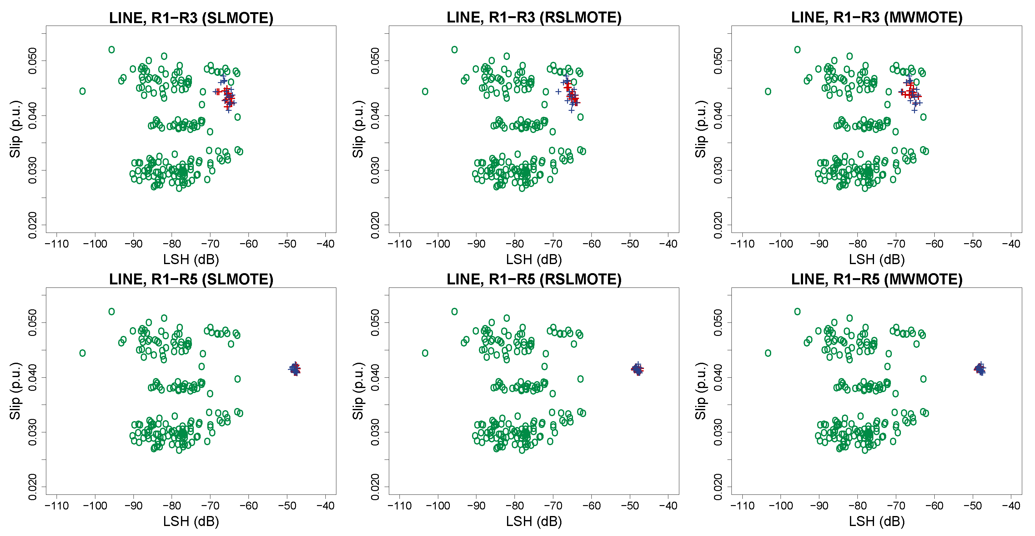
5.2. Effect on the Feature Subspace

After the feature selection stage, the IR is improved by the generation of synthetic data for the minority class using the different techniques previously described: SLSMOTE, RSLSMOTE, and MWMOTE. The balanced datasets are shown in Figure 6 and Figure 7. The first figure is for the motor line-fed case, and the second is for the inverter-fed case. The LSH fault feature vs. the motor slip is represented in all these figures for different failure severities. The different rotor conditions are depicted as follows: healthy case (O); original rotor fault data (+); synthetic rotor fault data (+).

In both figures, the LSH feature is represented vs. the motor slip. In the first row, the following two-rotor conditions are represented: healthy or R1 and intermediate severity or R3. In the second row, these two conditions are plotted: healthy or R1 and fully broken bar or R5. In all cases, the healthy observations outnumber the faulty ones, producing an IR of 12.

The resampling results for each algorithm are shown with red markers for each algorithm. The synthetic data generated with the SMOTE technique for the line supply case shows dispersed decision boundaries for the two-rotor severity (R3 and R5). However, with Safe-Level SMOTE and Relocating Safe-Level SMOTE variants, this does not happen. In the inverter-fed case, the results are quite similar.

5.3. Classification Stage

After balancing the datasets, three classification techniques are trained: Support Vector Machine (SVM) with Gaussian kernel as a radial basis function, Adaptive Boosting (AdaBoost), and instance-based k-nearest Neighbors (k-NN). The tuning parameters are $C=1$ for SVM, the number of neighbours for k-NN, and SMOTE set to $k=5$. Previously, different combinations of tuning parameters were explored during the parameter tuning procedure. The amount of oversampling is predetermined from the beginning for the imbalanced ratios indicated in Table 2.

6. Discussion

The twelve case studies are summarized in Table 2, while

Table 3. Classification results with feature selection and oversampling with SLSMOTE, RSLSMOTE, and MWMOTE.

Classifier	Supply	Case Number	Severity	Imbalance Ratio (IR)	AUC (%)	p-Value	Gmean1 (%)
SVM	Line-fed	1	R3	12	$97\pm 2.55$	$0.085$	$98\pm 1.58$
	Line-fed	2	R3	7	$97\pm 2.52$	$0.251$	$97\pm 2.63$
	Line-fed	3	R3	3	$97\pm 1.36$	$0.651$	$97\pm 2.14$
	Line-fed	4	R5	12	$100\pm 0.00$	$0.156$	$100\pm 0.00$
	Line-fed	5	R5	7	$100\pm 0.00$	$0.746$	$100\pm 0.00$
	Line-fed	6	R5	3	$100\pm 0.00$	$0.365$	$100\pm 0.00$
	Inverter	7	R3	12	$97\pm 2.11$	$0.711$	$97\pm 2.77$
	Inverter	8	R3	7	$96\pm 1.23$	<0.01	$97\pm 2.98$
	Inverter	9	R3	3	$96\pm 2.58$	<0.01	$97\pm 2.73$
	Inverter	10	R5	12	$100\pm 0.00$	$0.411$	$100\pm 0.00$
	Inverter	11	R5	7	$100\pm 0.00$	$0.709$	$100\pm 0.00$
	Inverter	12	R5	3	$100\pm 0.00$	$0.177$	$100\pm 0.00$
AdaBoost	Line-fed	1	R3	12	$97\pm 1.23$	$0.785$	$98\pm 1.42$
	Line-fed	2	R3	7	$97\pm 2.58$	$0.150$	$97\pm 2.40$
	Line-fed	3	R3	3	$98\pm 1.32$	$0.255$	$98\pm 1.84$
	Line-fed	4	R5	12	$100\pm 0.00$	$0.456$	$100\pm 0.00$
	Line-fed	5	R5	7	$100\pm 0.00$	$0.606$	$100\pm 0.00$
	Line-fed	6	R5	3	$100\pm 0.00$	$0.865$	$100\pm 0.00$
	Inverter	7	R3	12	$97\pm 1.10$	$0.545$	$97\pm 2.66$
	Inverter	8	R3	7	$97\pm 1.23$	<0.01 *	$97\pm 2.09$
	Inverter	9	R3	3	$98\pm 2.58$	<0.01 *	$97\pm 2.20$
	Inverter	10	R5	12	$100\pm 0.00$	$0.811$	$100\pm 0.00$
	Inverter	11	R5	7	$100\pm 0.00$	$0.709$	$100\pm 0.00$
	Inverter	12	R5	3	$100\pm 0.00$	$0.387$	$100\pm 0.00$
k-NN	Line-fed	1	R3	12	$97\pm 1.02$	$0.113$	$98\pm 1.88$
	Line-fed	2	R3	7	$96\pm 2.52$	$0.852$	$97\pm 2.81$
	Line-fed	3	R3	3	$97\pm 2.02$	$0.673$	$97\pm 2.88$
	Line-fed	4	R5	12	$98\pm 1.56$	$0.555$	$100\pm 0.00$
	Line-fed	5	R5	7	$100\pm 0.00$	$0.143$	$100\pm 0.00$
	Line-fed	6	R5	3	$100\pm 0.00$	$0.861$	$100\pm 0.00$
	Inverter	7	R3	12	$97\pm 1.10$	$0.219$	$97\pm 2.97$
	Inverter	8	R3	7	$95\pm 3.32$	<0.01 *	$97\pm 2.62$
	Inverter	9	R3	3	$96\pm 3.88$	<0.01	$96\pm 3.66$
	Inverter	10	R5	12	$100\pm 0.00$	$0.815$	$100\pm 0.00$
	Inverter	11	R5	7	$100\pm 0.00$	$0.113$	$100\pm 0.00$
	Inverter	12	R5	3	$100\pm 0.00$	$0.770$	$100\pm 0.00$

* Outcome of the test from pairwise performance where MWMOTE outperforms the rest.

presents the metrics used to evaluate the classification results of these cases. The performance of three classification algorithms is compared with datasets obtained after variable selection and class balancing using three oversampling algorithms. The comparison metrics were obtained through a 10-fold cross-validation process and were used for the comparative study of imbalanced classes. The metrics used for comparison are Area Under the ROC Curve (AUC) and G-mean1. AUC is derived from ROC analysis, which evaluates the performance of classifiers by plotting the True Positive Rate against the False Positive Rate while varying a score threshold. It is a scalar value representing the probability that a classifier performs better at classifying a fault instance over a healthy one, providing a single score for evaluating which algorithm is better on average. $G_{mean1}$ is used to evaluate the relative balance of classifier performance on all classes, computed as negative (Healthy) and positive (Fault):

$$G_{mean1}=\sqrt{TPR\times TNR},$$

(10)

where $TPR$ and $TNR$ are True Positive Rate and True Negative Rate, respectively.

For study cases 8 and 9, the combination of MWMOTE for class balancing and the AdaBoost classifiers performs better than the rest of the oversampling algorithms and classifiers. These cases correspond to the motor fed by inverter and intermediate inverter feeding, intermediate fault severity (R3), and imbalance ratios IR = 7 and IR = 3, respectively. However, when the imbalance ratio increases, every classifier and oversampling tool performs quite similarly, i.e., no statistical significance is found in their results. The statistical significance is checked with the Holm test. This test is applied for a pairwise performance among each oversampling approach whose p-values are shown in Table 3. The outcome is to reject the null hypothesis when this p-value falls below a threshold. This outcome implies that the corresponding SMOTE extension is outperformed by the remaining ones. This situation is highlighted with an asterisk in the p-value and found that only happens for the MWMOTE approach. Studies 4–6 and 10–12 cover both power sources, the maximum fault severity (R5), and all class imbalance rates. The classification metrics obtained are good for the various combinations of oversampling techniques and classification algorithms.

7. Conclusions

This article reviews and applies several resampling techniques for diagnosing rotor faults in line-fed and inverter-fed induction motors. These resampling techniques are SMOTE extensions and produce synthetic observations belonging to the minority fault class for balancing training sets and improving the synthetic data generation according to boundary area behavior.

The evaluation of the classifier performance with the metrics $AUC$ and $G_{mean1}$ metrics shows that for the highest fault severity of the broken rotor bar fault (R5), all resampling techniques considered have similar behavior, which implies that in terms of performance, any of them can obtain successful diagnostic results independent of the motor power supply and the imbalanced ratio analyzed.

Therefore, by incorporating any of these oversampling techniques into the diagnosis methodology to predict the rotor’s condition, it is possible to construct a more precise and robust diagnosis of the rotor faults of inverter-powered induction motors with small and unbalanced data.

In addition, from this experimental study, the authors observed that one area of exploration is the application of these oversampling methods to more incipient rotor breakages, where the feature differences regarding the healthy class are much more reduced.

References

1. Park, Y.; Jeong, M.; Bin Lee, S.; Teska, M.; Antonino-Daviu, J.A. Influence of Blade Pass Frequency Vibrations on MCSA-Based Rotor Fault Detection of Induction Motors. IEEE Trans. Ind. Appl. 2017, 53, 2049–2058. [Google Scholar] [CrossRef]
2. Zhou, Z.J.; Hu, C.H.; Wang, W.B.; Zhang, B.C.; Xu, D.L.; Zheng, J.F. Condition-based maintenance of dynamic systems using online failure prognosis and belief rule base. Expert Syst. Appl. 2012, 39, 6140–6149. [Google Scholar] [CrossRef]
3. Pons-Llinares, J.; Antonino-Daviu, J.; Roger-Folch, J.; Morinigo-Sotelo, D.; Duque-Perez, O. Mixed eccentricity diagnosis in Inverter-Fed Induction Motors via the Adaptive Slope Transform of transient stator currents. Mech. Syst. Signal Process. 2014, 48, 423–435. [Google Scholar] [CrossRef]
4. Benbouzid, M.E.H. A review of induction motors signature analysis as a medium for faults detection. IEEE Trans. Ind. Electron. 2000, 47, 984–993. [Google Scholar] [CrossRef]
5. Cunha Palacios, R.; Da Silva, I.; Goedtel, A.; Godoy, W. A comprehensive evaluation of intelligent classifiers for fault identification in three-phase induction motors. Electr. Power Syst. Res. 2015, 127, 249–258. [Google Scholar] [CrossRef]
6. Prieto, M.D.; Cirrincione, G.; Espinosa, A.G.; Ortega, J.A.; Henao, H. Bearing fault detection by a novel condition-monitoring scheme based on statistical-time features and neural networks. IEEE Trans. Ind. Electron. 2013, 60, 3398–3407. [Google Scholar] [CrossRef]
7. Ghate, V.N.; Dudul, S.V. Cascade neural-network-based fault classifier for three-phase induction motor. IEEE Trans. Ind. Electron. 2011, 58, 1555–1563. [Google Scholar] [CrossRef]
8. Gonzalez-Jimenez, D.; del Olmo, J.; Poza, J.; Garramiola, F.; Madina, P. Data-Driven Fault Diagnosis for Electric Drives: A Review. Sensors 2021, 21, 4024. [Google Scholar] [CrossRef]
9. Gonzalez-Jimenez, D.; Del-Olmo, J.; Poza, J.; Garramiola, F.; Madina, P. Data-Driven Low-Frequency Oscillation Event Detection Strategy for Railway Electrification Networks. Sensors 2023, 23, 254. [Google Scholar] [CrossRef]
10. Gonzalez-Jimenez, D.; del Olmo, J.; Poza, J.; Garramiola, F.; Sarasola, I. Machine Learning-Based Fault Detection and Diagnosis of Faulty Power Connections of Induction Machines. Energies 2021, 14, 4886. [Google Scholar] [CrossRef]
11. Martin-Diaz, I.; Morinigo-Sotelo, D.; Duque-Perez, O.; Romero-Troncoso, R.J. Early fault detection in induction motors using AdaBoost with imbalanced small data and optimized sampling. IEEE Trans. Ind. Appl. 2016, 53, 3066–3075. [Google Scholar] [CrossRef]
12. Niu, G.; Dong, X.; Chen, Y. Motor Fault Diagnostics Based on Current Signatures: A Review. IEEE Trans. Instrum. Meas. 2023, 72, 1–19. [Google Scholar] [CrossRef]
13. Rivera, W.A. Noise Reduction A Priori Synthetic Over-Sampling for class imbalanced data sets. Inform. Sci. 2017, 408, 146–161. [Google Scholar] [CrossRef]
14. Zhang, T.; Chen, J.; Li, F.; Zhang, K.; Lv, H.; He, S.; Xu, E. Intelligent fault diagnosis of machines with small & imbalanced data: A state-of-the-art review and possible extensions. ISA Trans. 2022, 119, 152–171. [Google Scholar] [CrossRef] [PubMed]
15. Kliman, G.; Stein, J. Methods of motor current signature analysis. Electr. Mach. Power Syst. 1992, 20, 463–474. [Google Scholar] [CrossRef]
16. Martin-Diaz, I.; Morinigo-Sotelo, D.; Duque-Perez, O.; Delgado-Arredondo, P.; Camarena-Martinez, D.; Romero-Troncoso, R. Analysis of various inverters feeding induction motors with incipient rotor fault using high-resolution spectral analysis. Electr. Power Syst. Res. 2017, 152, 18–26. [Google Scholar] [CrossRef]
17. Bruzzese, C. Analysis and Application of Particular Current Signatures (Symptoms) for Cage Monitoring in Nonsinusoidally Fed Motors With High Rejection to Drive Load, Inertia, and Frequency Variations. IEEE Trans. Ind. Electron. 2008, 55, 4137–4155. [Google Scholar] [CrossRef]
18. Robnik-Sikonja, M.; Kononenko, I. Theoretical and empirical analysis of ReliefF and RReliefF. Mach. Learn. 2003, 53, 23–69. [Google Scholar] [CrossRef]
19. Kononenko, I.; Robnik-Sikonja, M.; Pompe, U. ReliefF for Estimation and Discretization of Attributes in Classification, Regression, and ILP Problems; IOS Press: Amsterdam, The Netherlands, 1996; Volume 35. [Google Scholar]
20. Murcia-Sepúlveda, N.; Cruz-Duarte, J.M.; Martin-Diaz, I.; Garcia-Perez, A.; Rosales-García, J.J.; Avina-Cervantes, J.G.; Correa-Cely, C.R. Fractional Calculus-Based Processing for Feature Extraction in Harmonic-Polluted Fault Monitoring Systems. Energies 2019, 12, 3736. [Google Scholar] [CrossRef]
21. Chawla, N.V.; Bowyer, K.W.; Hall, L.O.; Kegelmeyer, W.P. SMOTE: Synthetic minority over-sampling technique. J. Artif. Intell. Res. 2002, 16, 321–357. [Google Scholar] [CrossRef]
22. Bunkhumpornpat, C.; Sinapiromsaran, K.; Lursinsap, C. Safe-Level-SMOTE: Safe-Level-Synthetic Minority Over-Sampling TEchnique for Handling the Class Imbalanced Problem. In Proceedings of the Advances in Knowledge Discovery and Data Mining, Bangkok, Thailand, 27–30 April 2009; Theeramunkong, T., Kijsirikul, B., Cercone, N., Ho, T.B., Eds.; Springer: Berlin/Heidelberg, Germany, 2009; pp. 475–482. [Google Scholar]
23. Siriseriwan, W.; Sinapiromsaran, K.; Tipawanna, M.; Bunkhumpornpat, C.; Keatruangkamala, K. The effective redistribution for imbalance dataset: Relocating Safe-level SMOTE with minority outcast handling. Chiang Mai J. Sci. 2016, 43, 1288–1300. [Google Scholar]
24. Barua, S.; Islam, M.M.; Yao, X.; Murase, K. MWMOTE—Majority weighted minority oversampling technique for imbalanced data set learning. IEEE Trans. Knowl. Data Eng. 2014, 26, 405–425. [Google Scholar] [CrossRef]
Figure 1. Power spectral density of a measured stator current from a line-fed induction motor.
Applsci 14 07237 g001
Figure 2. Power spectral density of a measured stator current from an inverter-fed induction motor.
Applsci 14 07237 g002
Figure 3. Demonstration of the operation of the MWMOTE algorithm. A dataset from an inverter-fed motor is used. The green markers represent the majority class (healthy motor), and the blue markers represent the minority class (motor with failure). (a) Case with imbalanced classes; (b) synthetically balanced case (synthetically created markers are shown in red).
Applsci 14 07237 g003
Figure 4. Test bench employed in this research. (1) Induction motor; (2) magnetic powder brake and load control unit (3) custom-made hall effect sensor board; (4) DAQ board; (5) laptop and software; (6) inverters; (7) simulated broken rotor bars.
Applsci 14 07237 g004
Figure 5. Results of the feature selection with the ReliefF algorithm: a line-fed case at the (top) and an inverter-fed case at the (bottom) of the figure.
Applsci 14 07237 g005
Figure 6. Bidimensional feature scatterplot (slip and LSH) for synthetically balanced data from line supply with the resampling techniques: Safe Level-SMOTE (SLMOTE), Relocating Safe Level SMOTE (RSLMOTE), and Majority weighted minority oversampling technique (MWMOTE). An imbalanced ratio of 12. Top figures: R3 rotor severity. Bottom figures: R5 rotor severity. The different rotor conditions are depicted as follows: healthy case (O); original rotor fault data (+); synthetic rotor fault data (+).
Applsci 14 07237 g006
Figure 7. Bidimensional feature scatterplot (slip and LSH) for synthetically balanced data from inverter-based supply with the resampling techniques: Safe Level-SMOTE (SLMOTE), Relocating Safe Level SMOTE (RSLMOTE), and Majority weighted minority oversampling technique (MWMOTE). An imbalanced ratio of 12. Top figures: R3 rotor severity. Bottom figures: R5 rotor severity. The different rotor conditions are depicted as follows: healthy case (O); original rotor fault data (+); synthetic rotor fault data (+).
Applsci 14 07237 g007