Reduced Element for Adaptive Finite Element Analysis of First-Order IVP with Built-in Error Estimator in Maximum Norm

Abstract

This paper proposes a novel yet simple approach to the adaptive finite element (FE) analysis of the first-order Initial Value Problems (IVPs) in the maximum norm by introducing the reduced element technique. In the present approach, the FE solution u^h of the conventional Galerkin element of degree m + 1 is decomposed into two parts: a reduced solution $u_{\mathrm{R}}^h$ from the reduced element of degree m obtained by ignoring the highest degree term of u^h, and a built-in point-wise error estimator ${\epsilon }_{\mathrm{R}}^h$ directly given by the ignored term. Since the end node solutions of the reduced element are inherited from the full order element, it gains O(h^2m+2) accuracy and achieves a nodal/element accuracy ratio as high as two, which greatly enhances its adaptive capability regarding solving IVPs on long time domains. The related error analysis is addressed and a complete adaptivity algorithm is given. Typical numerical examples of both linear and nonlinear IVPs of both single and systems of equations are presented to show the validity and effectiveness of the proposed approach.

1. Introduction

First-order Initial Value Problems (IVPs) play a fundamental role in theoretical and numerical analyses of physical and engineering problems [1,2,3,4,5]. Theoretically, any higher order ordinary differential equations (ODEs) can equivalently be transformed into systems of first-order ODEs and hence successful numerical methods for the first-order IVPs can also be applied to the Boundary Value Problems (BVPs) in ODEs. Numerically, it is often easier to develop straightforward, flexible and robust methods since only the solution functions are solved for without the need to consider solution derivatives.

For adaptive analysis of the first-order IVPs, error estimation is required in certain kinds of norm. Instead of a thorough survey of various relevant numerical methods, the most used Runge–Kutta–Fehlberg method [3,6] is worth mentioning on account of its representativeness and the availability of algorithms for adaptive analysis. The conventional adaptive approach based on the Runge–Kutta method estimates the truncation errors of a fourth-order Runge–Kutta method using the solution of a fifth-order Runge–Kutta method. This approach is simple and effective and can effectively control the truncation errors to a certain extent. However, the solution obtained by this method is in a discrete form, and it is impossible to measure the errors by maximum norm, and it is difficult to use the $L^2$ norm as well. Moreover, this method is not A-stable for first-order IVPs [6], which flaws its flexibility and reliability. Although many research works on this method have been conducted to improve this method in recent years [7,8,9], the above-mentioned problems have not been fundamentally resolved.

The conventional Galerkin finite element method (FEM) [10,11,12] is a convenient and effective tool for both BVPs and IVPs [4,13,14,15,16,17,18,19]. Although, for the second-order equation of motion in structural dynamics analysis, the conventional Galerkin FEM can only generate conditionally stable algorithms, it can generate unconditionally stable algorithms if the second-order IVPs are transformed to the first-order IVPs in system of ODEs [13,17,20]. Specifically, characterized by piecewise polynomial spaces of degree $m$, the conventional Galerkin FEM for the first-order IVPs [13,17] can generate a one-step and A-stable method with $O(h^{m+1})$ accuracy within elements, and $O(h^{2m})$ accuracy at mesh points (element end nodes) [13] for nodal solutions ($h$ being the maximum element size), which is particularly advantageous for a procedure of the time integration type. Recently, the authors of this paper proposed a condensed Galerkin element [20] for the first-order IVPs, which has been proved to be able to produce exactly identical nodal solutions as the conventional element of degree $m+1$ for the IVPs with constant coefficients, and hence gains super-convergent nodal solutions of $O(h^{2m+2})$; i.e., $m$-degreed elements gain the nodal results of ($m+1$)-degreed elements.

For adaptive finite element (FE) analysis, unlike discrete methods, the FE method provides continuous solutions on the complete time domain and hence it is possible to employ an error estimator in the maximum norm, which is exclusively adopted in this paper. A more significant aspect of the FEM is its super-convergent nodal solutions, i.e., $O(h^{2m})$ for the conventional element or $O(h^{2m+2})$ for the condensed element, because the nodal solutions serve as the initial values for the next time-step (element) solution. However, as is well known, element accuracy is not the only criterion for overall performance. Based on numerous theoretical analyses and numerical experiments conducted by the authors, it has been identified that, for a reliable and robust adaptive FE analysis of the first-order IVPs with adaptive time-stepping (element sizing) controlled by the maximum norm, there are three crucial requirements for a high-performance algorithm to satisfy, described as follows.

• R1. The element should be unconditionally stable.

Otherwise, the element can hardly be viewed to be fully reliable and robust.

• R2. The element should gain high nodal/element convergence ratio.

This is to guarantee that the local (element) error estimate is reasonably reliable and the initial conditions for each new time-step (element) are of sufficiently high accuracy. Numerous numerical experiments have suggested that, especially for relatively long time domains, the ratio between the convergence orders at element end nodes and within elements is best up to two, i.e.,

$$\mathrm{Accuracy} \mathrm{ratio}\equiv {\displaystyle \frac{\mathrm{nodal} \mathrm{convergence} \mathrm{order}}{\mathrm{element} \mathrm{convergence} \mathrm{order}}}=2.$$

(1)

In other words, for an element of degree $m$ with a convergence $O(h^{m+1})$ on the element, the nodal convergence order would best reach to $O(h^{2m+2})$.

• R3. The element should be equipped with a reliable point-wise error estimator.

With the requirement R2 satisfied, a super convergent solution with accuracy at least one order higher than the FE solution should be available to serve as an effective error estimator in the maximum norm.

Among the above three requirements, both the conventional and condensed elements satisfy R1, only the condensed element satisfies R2, and neither satisfies R3 unless an extra higher order super-convergent solution is available or constructed, which is a severe challenge to confront.

Based on the conventional element model, this paper proposes a novel approach, named the “reduced element” technique, which satisfies all the three requirements in a simple, direct, and straightforward way without the need for an additional separate computation to find an error estimator. Simply speaking, in this approach, suppose the adaptive analysis is aimed at an FE solution of $m$-degreed elements with the pointwise errors required to satisfy the user preset tolerance $T_l$; we simply solve the problem by using elements of one order higher, i.e., degree $m+1$, and then after the FE solution, we extract, on each element, the results up to degree $m$ as the target solution with the highest ordered (degree $m+1$) term used as a pointwise error estimator. Since the target solution is from the elements of reduced order (degree m) extracted from the elements of full order (degree $m+1$), it is simply called the “reduced element” technique.

2. First-Order IVP and Galerkin Method

2.1. Model Problem

For conciseness and brevity, the problem considered in this paper is focused on the following first-order linear ODE with constant coefficient $q$:

$$\{\begin{array}{l}{u}^{\prime }(t)+qu(t)=f(t),\hspace{1em}\hspace{1em}0<t\le \overline{T}\\ u(0)=u_0\end{array},$$

(2)

where $u(t)$ is the solution to be solved for with the uniqueness being assumed, $f(t)$ is a prescribed function, $u_0$ is the initial value, and $\overline{T}$ is the terminus of the time domain. The case of the nonlinear IVP will be addressed later in this paper. Although the model problem is of a single ODE, the approach presented in this paper is well applicable to systems of such ODEs.

2.2. Galerkin Method

To construct a Galerkin weak form, define bilinear and linear forms, respectively, as follows:

$$a(u,v)={\displaystyle {\int }_0^{\overline{T}}v(u^{\prime }+qu)\mathrm{d}t}, (f,v)={\displaystyle {\int }_0^{\overline{T}}vf\mathrm{d}t}.$$

(3)

where $v$ is the test function. Let $H_u^1$ denote the trial space formed by all the functions on the time domain which satisfy the initial condition in Equation (2) and are square integrable up to the first derivative, and let $H_v^0$ denote the test space formed by all the functions which are square integrable themselves. Then the Galerkin method for the IVP in Equation (2) is to find $u\in H_u^1$ such that

$$a(u,v)=(f,v),\hspace{1em}\forall v\in H_v^0.$$

(4)

3. Conventional Galerkin Element

3.1. Galerkin Finite Element

In Galerkin FE analysis, the trial space $S_{u,m}^h\subset H_u^1$ is formed by polynomials of degree m on each element, and the test space $S_{v,m-1}^h\subset H_v^0$ is formed by polynomials of degree $m-1$ on each element. Since the conventional element model is of the one-step type and the whole solution on the mesh can be obtained element by element in a recursive fashion, it suffices to consider only the first element $(t_0,t_1)\equiv (0,h)$ as the time domain [20].

For convenience, the Legendre-polynomial-based hierarchical shape functions are employed in this paper with the trial function $u^h$ of degree $m$ and the test function $v^h$ of degree $m-1$ respectively expressed as

$$u^h={\overline{N}}_1(t)u_1^h+{\displaystyle {\sum }_{k=2}^m{\widehat{N}}_k(t)u_{k+1}^h}+{\overline{N}}_2(t)u_2^h, v^h={\displaystyle \sum _{i=1}^m{N}_i^{*}(t)v_i^h}.$$

(5)

For the trial function $u^h$, the shape functions of the element two end nodes are usual linear functions:

$${\overline{N}}_1=1-{\displaystyle \frac{t}{h}},\hspace{1em}{\overline{N}}_2={\displaystyle \frac{t}{h}},$$

(6)

and the internal ‘bubble’ shape functions of degree $k(\ge 2)$ are taken as

$${\widehat{N}}_k(t)=P_{k_0}(x)-P_k(x),\hspace{1em}k=2,3,\dots ,m,$$

(7)

where $P_k(x)$ is the standard Legendre polynomial of degree $k$ with $x=-1+2t/h$ and

$$k_0=\{\begin{array}{l}0,\hfill \\ 1,\hfill \end{array}\hspace{1em}\begin{array}{c}k=2,4,6,\dots \\ k=3,5,7,\dots \end{array}.$$

(8)

To be specific, the expanded forms of the leading shape functions are

$${\widehat{N}}_2(t)=3(1-x^2)/2, {\widehat{N}}_3(t)=5x(1-x^2)/2, {\widehat{N}}_4(t)=5(1-x^2)(1+7x^2)/8,\dots .$$

(9)

For the test function $v^h$, the shape functions simply adopt the Legendre polynomials as follows:

$$N_i^{*}(t)=P_{i-1}(x),\hspace{1em}i=1,2,\dots ,m.$$

(10)

Note that the test function $v^h$ takes a polynomial of one degree lower than the trial function $u^h$, and is independent on each element while the trial function $u^h$ is continuous at common nodes, i.e., at mesh points. Thus, the conventional Galerkin finite element solution is to find $u^h\in S_{u,m}^h$ such that

$$a(u^h,v^h)=(f,v^h),\hspace{1em}\forall v^h\in S_{v,m-1}^h.$$

(11)

3.2. Convergence Property

The convergence property of the above conventional elements for the first-order IVPs has been mathematically analyzed by Hulme [13] with the following error bounds obtained:

$$\begin{gathered} \underset{0\le t\le \overline{T}}{\max }\left|u(t)-u^h(t)\right|\le C{h}^{m+1} \mathrm{on} \mathrm{elements}, \\ \left|u_i-u_i^h\right|\le C{h}^{2m} \mathrm{at} \mathrm{mesh} \mathrm{point} i(=0,1,\dots ,N_e). \end{gathered}$$

(12)

where $N_e$ is the total number of elements. Further, it has also been proved that the FEM with such conventional elements is A-stable. These properties are crucial to the present work and will be utilized in this paper.

In the following, unless otherwise mentioned, the term ‘nodal solution’ is used exclusively to refer to the ‘solution at element end nodes’, i.e., at mesh points. Note that this class of elements gain super-convergence $O(h^{2m})$ for nodal solutions, which is a very desirable advantage for a numerical method of the time-integration type for IVPs. On the other hand, however, the accuracy ratio of the conventional element is $2m/(m+1)<2$ and it is found that for relatively long time domain problem, the accumulated nodal errors could be prominent and uncontrollable (See Section 6.2).

4. Reduced Element

4.1. Sturcture of the Reduced Element

Let $u^h$ denote the FE solution of the conventional element of degree $m+1$, which hereinafter will be called the ‘full order solution’ (or simply ‘full solution’). Also let $u_{\mathrm{R}}^h$ denote the associated solution of the reduced element of degree $m$, which will be called the ‘reduced order solution’ (or simply ‘reduced solution’). As mentioned above, the extraction of the reduced solution from the full solution is as follows: after the full order solution $u^h$ has been obtained, it is reduced to the solution $u_{\mathrm{R}}^h$ of one order lower by ignoring the ($m+1$)-degreed term. With the hierarchical shape functions employed, it is extremely simple to extract the reduced solution simply by ignoring the term ${\widehat{N}}_{m+1}(t)u_{m+2}^h$ in Equation (5) as follows:

$$u_{\mathrm{R}}^h={\overline{N}}_1(t)u_1^h+{\displaystyle {\sum }_{k=2}^m{\widehat{N}}_k(t)u_{k+1}^h}+{\overline{N}}_2(t)u_2^h.$$

(13)

The term ${\widehat{N}}_{m+1}(t)u_{m+2}^h$ is not thrown away and will serve as an error term ${\epsilon }_{\mathrm{R}}^h=u^h-u_{\mathrm{R}}^h$, which will be further explained later. Also note that $u_{\mathrm{R}}^h$ is not a genuine FE solution since it is not directly solved for by an FE procedure and it is simply a certain kind of $m$-degreed polynomial interpolation to the full order solution $u^h$. Therefore, the structure of the full solution is viewed to be composed of two parts: the reduced solution $u_{\mathrm{R}}^h$ and an error estimator ${\epsilon }_{\mathrm{R}}^h$. Figure 1 schematically shows the structure of the reduced linear element.

4.2. Error Analysis

Since the full order solution $u^h$ of degree $m+1$ is a conventional FE solution, and hence, from Equation (12), it gains convergence $O(h^{m+2})$ on element and $O(h^{2m+2})$ at element end nodes, i.e.,

$$\begin{gathered} \underset{0\le t\le \overline{T}}{\max }\left|u(t)-u^h(t)\right|\le C{h}^{m+2} \mathrm{on} \mathrm{elements}, \\ \left|u_i-u_i^h\right|\le C{h}^{2m+2} \mathrm{at} \mathrm{mesh} \mathrm{point} i(=0,1,\dots ,N_e). \end{gathered}$$

(14)

To estimate the error in the reduced order solution $u_{\mathrm{R}}^h$, it is easy to see that

$$\left|u-u_{\mathrm{R}}^h\right|=\left|u-u^h+u^h-u_{\mathrm{R}}^h\right|\le \left|u-u^h\right|+\left|u^h-u_{\mathrm{R}}^h\right|.$$

(15)

It follows from Equation (14) that the first term $\left|u-u^h\right|$ in Equation (15) is $O(h^{m+2})$. And, the error $\left|u^h-u_{\mathrm{R}}^h\right|$ of the second term in Equation (15) is purely a polynomial interpolation error, which is well known to be of $O(h^{m+1})$. Thus, it is concluded that

$$\begin{gathered} \underset{0\le t\le \overline{T}}{\max }\left|u(t)-u_{\mathrm{R}}^h(t)\right|\le C{h}^{m+1} \mathrm{on} \mathrm{elements}, \\ \left|u_i-u_{\mathrm{R},i}^h\right|\le C{h}^{2m+2} \mathrm{at} \mathrm{end} \mathrm{nodes}. \end{gathered}$$

(16)

Note that the nodal solutions of the reduced element are inherited from the full order solutions of the full order element, which ideally raises the accuracy ratio to 2 for the reduced element. Furthermore, the above error analysis validates the fact that the full solution, since it is at least one order higher than the reduced solution, is well qualified to serve as a pointwise error estimator for the reduced solution, which is in a very simple form as

$${\epsilon }_{\mathrm{R}}^h(t)={\widehat{N}}_{m+1}(t)u_{m+2}^h.$$

(17)

Without pointwise searching, the maximum error can be directly calculated as

$$\underset{e}{\max }\left|{\epsilon }_{\mathrm{R}}^h(t)\right|=\max \left|{\widehat{N}}_{m+1}(t)\right|\cdot \left|u_{m+2}^h\right| \mathrm{with} \max \left|{\widehat{N}}_2(t)\right|=3/2, \max \left|{\widehat{N}}_3(t)\right|=5\sqrt{3}/9,\dots .$$

(18)

4.3. Main Ideas

In this subsection, the main ideas for the reduced element are illustrated by a sample example from the practical computation. Without losing generality, the equation of motion with initial displacement $u(0)=0$ is solved respectively by a quadratic and linear element on an initial step $[0,h]$ with the step-size (element length) $h=3.5$. Related solutions are shown in Figure 2, in which $u$ is the exact solution, $u_{\mathrm{L}}^h$ and $u_{\mathrm{Q}}^h$ denote the solutions of the conventional linear and quadratic elements respectively, and $u_{\mathrm{R}}^h$ is the solution of the reduced linear element. From Figure 2, the following observations can be made.

For the conventional linear element solution $u_{\mathrm{L}}^h$, it is seen that the largest error occurs at the second end node. This is very unfavorable since, for an adaptive time-stepping approach, if the nodal errors happen to be exactly equal to the required tolerance, then there is no room for the errors to further accumulate in the subsequent solution steps, making the error control aborted. For the conventional quadratic element solution $u_{\mathrm{Q}}^h$, although the overall errors have been tremendously reduced, the maximum error still occurs at second end node, and the similar failure mentioned above may be inescapable either. However, for the solution $u_{\mathrm{R}}^h$ of the reduced linear element, which is simply a linear interpolation to the quadratic solution, it is seen that there are a couple of desirable properties and advantages:

• The reduced solution $u_{\mathrm{R}}^h$ is not a standard linear element solution: its interior solution is $O(h^2)$ accuracy, but its nodal solution is inherited from $u_{\mathrm{Q}}^h$ and attains $O(h^4)$ accuracy, which ideally makes the accuracy ratio exactly 2;
• The maximum error occurs within the element, leaving the nodal errors virtually negligible, which provides sufficiently accurate initial values for the subsequent solution steps, and hence greatly slows down accumulation of nodal errors on a long time domain;
• Since the full order solution $u_{\mathrm{Q}}^h$ is much closer to the exact solution u, i.e., one order higher than the reduced solution $u_{\mathrm{R}}^h$, the full order solution $u_{\mathrm{Q}}^h$ can serve as a convenient and qualified error estimator for a point wise error estimate over the reduced solution $u_{\mathrm{R}}^h$.

5. Adaptive Algorithm

5.1. Objective of Adaptivity

The adaptive FE analysis in this paper is of the adaptive time-stepping (element size) type, i.e., the analysis is implemented element by element with each element size adaptively adjusted. Let $e$ denote a representative element. The ultimate objective of the adaptive analysis in this paper is to find an optimal element size $h$ for each element $e$, such that the reduced solution $u_{\mathrm{R}}^h$ of the reduced element of degree $m$ obtained on the element $e$ satisfies the user-specified tolerance $T_l$ in the maximum norm:

$$\underset{e}{\max }\left|u-u_{\mathrm{R}}^h\right|\le T_l.$$

(19)

Since the exact solution $u$ is generally unknown, the full order solution $u^h$ of degree $m+1$ is used to replace $u$ for error checking, and Equation (19) becomes

$$\underset{e}{\max }\left|u^h-u_{\mathrm{R}}^h\right|=\underset{e}{\max }\left|{\epsilon }_{\mathrm{R}}^h\right|\le T_l.$$

(20)

Note that the above maximum error can be directly calculated as shown in Equation (18). Letting ${\overline{e}}_{\max }^{*h}$ and ${\overline{e}}_{\max }^h$ denote the estimated error ratio and true error ratio defined respectively by

$${\overline{e}}_{\max }^{*h}\equiv \underset{e}{\max }\left|{\epsilon }_{\mathrm{R}}^h\right|/T_l, {\overline{e}}_{\max }^h\equiv \underset{e}{\max }\left|u-u_{\mathrm{R}}^h\right|/T_l.$$

(21)

By introducing a pair of bounds for the estimated error ratios, the stopping criterion in Equation (20) is replaced in practical implementation by the following criteria

$${\overline{e}}_{\max }^{*h}\in ({\gamma }_l,{\gamma }_u).$$

(22)

In this paper, we simply take $({\gamma }_l,{\gamma }_u)=(0.1,0.85)$ throughout.

5.2. Element Size

In the adaptive process, if for any element Equation (22) is not satisfied, then a new element size is calculated by a formula proposed in Ref. [17] as follows:

$$h=h_0{\left({\displaystyle \frac{\alpha \cdot T_l}{\underset{e}{\max }\left|u^h-u_{\mathrm{R}}^h\right|}}\right)}^{{\displaystyle \frac{2}{2m+3}}},$$

(23)

where $h_0$ is the current element size and $\alpha \le 1$ is a safety factor and is set to $\alpha =0.8$ to match the upper bound ${\gamma }_u=0.85$ in this paper.

5.3. Adaptivity Algorithm

The adaptivity algorithm for the reduced element approach can be summarized as:

• Specify tolerance T_l, the degree m of the reduced element and the initial element size h₀;
• Solve for the FE solution u^h on the current element by using conventional element of degree m + 1;
• Extract the reduced solution $u_{\mathrm{R}}^h$ and calculate the maximum error ratio ${\overline{e}}_{\max }^{*h}$;
• If Equation (22) is satisfied, then move to the next element with current element h as the initial h₀, and return to Step 2;
• If Equation (22) is not satisfied, calculate a new element size h by using Equation (23), and return to Step (2);
• The above procedure is repeated until reaching the end of the time domain $\overline{T}$.

Note that the present paper employed the more stringent maximum norm rather than the more commonly used energy norm used in most adaptive analyses. Numerous numerical experiments show that the satisfaction of Equation (20) would indeed make Equation (19) also satisfied.

5.4. Nonlinear Problems

The first-order nonlinear problem is usually expressed as

$$u^{\prime }(t)=f(t;u).$$

(24)

Ref. [20] compared two iterative methods for FE analysis, i.e., direct iterative method and Newton’s iterative method, and concluded that Newton’s iterative method is superior to the direct iterative method. Therefore, in this paper, Newton’s method is employed to linearize Equation (24) and then the corresponding iterative formula for this method can be schematically written in the following form

$$u^{\prime }(t)+q(t)u(t)=q(t)\overline{u}(t)+f(t;\overline{u})\hspace{1em}\mathrm{with}\hspace{1em}q(t)={-{\displaystyle \frac{\partial f}{\partial u}}|}_{\overline{u}},$$

(25)

where, $\overline{u}$ is the known result from the previous iterative step. The adaptivity algorithm for nonlinear problems mostly remains the same as that in the previous subsection and the only modification is Step 2, where “Solve for the FE solution $u^h$” is replaced by “Solve for the nonlinear FE solution $u^h$”.

6. Numerical Examples

In this section, representative numerical examples are given to test the proposed algorithm. To eliminate any accuracy loss due to insufficient numerical precision, the computation of Section 6.1 and Section 6.2 are performed by using the symbolic software Maple 12 with a precision of 32 decimal digits (roughly equivalent to quadruple precision in Fortran language on a 32-bit PC) to guarantee the results faithfully reflect the developed theory. To show pure numerical implementation, Section 6.3 is computed by a Fortran 90 code with Gaussian quadrature and SOLVEBLOCK [21] package employed. In the practical computation, various tolerances $T_l$ ranging from ${10}^{-3}$ to ${10}^{-6}$ are adopted, and the linear ($m=1$) and cubic ($m=3$) reduced elements are employed for the presentation although other degreed elements have also been tested. For all the examples, the initial element size is taken as $h_0=0.5$.

6.1. An Illustrative Example

The first example is given to describe the detailed steps of the adaptive procedure, showing in particular how to form the FE matrix equation, how to estimate the maximum errors, and how to adjust the element size. The problem is the linearized Problem 3 in the next example, i.e.,

$$u^{\prime }+4tu=0,u(0)=1,u(t)=e^{-2t^2},0\le t$$

(26)

The objective is to solve for the solution on the first element $(0,h)$ with the element size $h$ being adaptively adjusted. The reduced linear element ($m=1$) is used as the final solution and, accordingly, the full element is a quadratic element, which can provide fourth-order nodal solutions (Equation (12)). From Equation (5), the trial and test functions are respectively as follows

$$u^h=\left(1-{\displaystyle \frac{t}{h}}\right)u_1^h+6\left(1-{\displaystyle \frac{t}{h}}\right)\left({\displaystyle \frac{t}{h}}\right)u_3^h+\left({\displaystyle \frac{t}{h}}\right)u_2^h,\hspace{1em}{v}^h=v_1^h+\left(-1+{\displaystyle \frac{2t}{h}}\right)v_2^h.$$

(27)

Then the bilinear form in Equation (11) is

$$a^e(u^h,v^h)=\left\{v_1^h{v}_2^h\right\}\left[\begin{array}{ccc}{\displaystyle \frac{2h^2}{3}}-1& 2h^2& {\displaystyle \frac{4h^2}{3}}+1\\ 0& {\displaystyle \frac{2h^2}{5}}-2& {\displaystyle \frac{2h^2}{3}}\end{array}\right]\left\{\begin{array}{c}{u}_0\\ u_3^h\\ u_2^h\end{array}\right\}.$$

(28)

Note that by introducing the initial condition, $u_1^h$ has been replaced by $u_0$. Then, from the arbitrariness of $v_1^h$ and $v_2^h$, the matrix equation can be derived based on Equation (11) as

$$\left[\begin{array}{cc}2h^2& {\displaystyle \frac{4}{3}}{h}^2+1\\ {\displaystyle \frac{2h^2}{5}}-2& {\displaystyle \frac{2h^2}{3}}\end{array}\right]\left\{\begin{array}{c}{u}_3^h\\ u_2^h\end{array}\right\}=\left\{\begin{array}{c}1-{\displaystyle \frac{2h^2}{3}}\\ 0\end{array}\right\}{u}_0,$$

(29)

the solution of which is

$$u_3^h={\displaystyle \frac{-10h^4/3+5h^2}{6h^4+17h^2+15}}{u}_0,\hspace{1em}{u}_2^h={\displaystyle \frac{2h^4-13h^2+15}{6h^4+17h^2+15}}{u}_0.$$

(30)

Note that $u_2^h$ is the FE solution at second end node of the element. It is easily seen that

$$\left|{\displaystyle \frac{2h^4-13h^2+15}{6h^4+17h^2+15}}\right|<1 \mathrm{when} h>0,$$

(31)

which means the element is unconditionally stable. To see the local (truncated) error of the full FE solution, the series expansion of the true error gives

$$u(h)-u^h(h)=u(h)-u_2^h={\displaystyle \frac{2}{15}}{h}^6+O(h^7) \mathrm{with} u_0=1.$$

(32)

Note that the local error is of order 6, which is one order higher than it is estimated in Equation (12). This is because that the series expansion of the exact solution $e^{-2t^2}=1-2h^2+2h^4-4h^6/3+O(h^7)$ lacks the term of order 5. With the full FE (conventional element) solution $u^h$ obtained, the reduced solution $u_{\mathrm{R}}^h$ (Equation (13)), the estimated error term ${\epsilon }_{\mathrm{R}}^h$ (Equation (17)) and the estimated maximum error $\max \left|{\epsilon }_{\mathrm{R}}^h\right|$ (Equation (18)) are, respectively, as follows:

$$u_{\mathrm{R}}^h=\left(1-{\displaystyle \frac{t}{h}}\right)u_0^h+\left({\displaystyle \frac{t}{h}}\right)u_2^h,\hspace{1em}{\epsilon }_{\mathrm{R}}^h=6\left(1-{\displaystyle \frac{t}{h}}\right)\left({\displaystyle \frac{t}{h}}\right)u_3^h,\hspace{1em}\max \left|{\epsilon }_{\mathrm{R}}^h\right|={\displaystyle \frac{3}{2}}{u}_3^h.$$

(33)

Now we are in a position to implement the adaptive FE analysis for the first element with the preset tolerance $T_l=0.001$.

Taking the initial element size $h_0=0.5$ and setting the initial value $u_0=1$, the following numerical results can be obtained from Equation (30)

$$u_3^h=0.05307856,\hspace{1em}{u}_2^h=0.60509554.$$

(34)

The true error at the right end node is $u(h)-u_2^h=0.00143511$. It would be informative to calculate the same problem setting by using the fourth-order Runge–Kutta method, which yields the value $0.60416667$ at $t=0.5$ with the true error being 0.00236399, and turns out to be less accurate than the fourth-ordered solution of the quadratic element.

The true maximum error and the estimated error on the element are, respectively,

$$\underset{0\le t\le h}{\max }\left|u(t)-u_{\mathrm{R}}^h(t)\right|=0.08150929,\hspace{1em}\underset{0\le t\le h}{\max }\left|{\epsilon }_{\mathrm{R}}^h(t)\right|=3u_3^h/2=0.07961783.$$

(35)

Since $\underset{0\le t\le h}{\max }\left|{\epsilon }_{\mathrm{R}}^h(t)\right|>T_l$, the formula in Equation (23) is used to generate a new element size

$$h=0.5\times {\left({\displaystyle \frac{0.8\times 0.001}{0.07961783}}\right)}^{{\displaystyle \frac{2}{5}}}=0.79396591.$$

(36)

With this new $h$, updated nodal values are calculated

$$u_3^h=0.00207757,\hspace{1em}{u}_2^h=0.98747147.$$

(37)

The subsequent computational steps are summarized in

Table 1. Adaptive steps of the first element of Section 6.1 ($T_l=0.001$).

Adaptive Step	Element Size	Nodal Values		True Error at Right End Node	Estimated Maximum Element Error	True Maximum Element Error
k	h	${\mathit{u}}_3^{\mathit{h}}$	${\mathit{u}}_2^{\mathit{h}}$	$\mathit{u}(\mathit{h})-{\mathit{u}}_2^{\mathit{h}}$	$\underset{0\le \mathit{t}\le \mathit{h}}{\mathbf{max}}\left|{\mathit{\epsilon }}_{\mathbf{R}}^{\mathit{h}}(\mathit{t})\right|$	$\underset{0\le \mathit{t}\le \mathit{h}}{\mathbf{max}}\left|\mathit{u}-{\mathit{u}}_{\mathbf{R}}^{\mathit{h}}\right|$
1	0.5	0.05307856	0.60509554	0.144 × 10−2	0.079618	0.081509
2	0.79396591	0.00207757	0.98747147	0.331 × 10−7	0.003116	0.003117
3	0.04608710	0.00070531	0.99576097	0.127 × 10−8	0.001058	0.001058
4	0.04121241	0.00056443	0.99660884	0.652 × 10−9	0.000847	0.000847

, from which it can be seen that although the initial element size $h=0.5$ is very large, it converges very fast, and after 4 adaptive steps, both the estimate error and the true error satisfy the required error tolerance $0.85T_l$ (Equation (22)). It can also be seen that the maximum error estimation of the reduced element is very accurate, and the nodal errors are much smaller than the element errors, to guarantee the provision of an initial value of higher order accuracy (with the error 0.652 × 10⁻⁹) for the next time element.

6.2. Batch of 6 Numerical Examples

In this part, all the six problems originally solved in Ref. [13] by using the Galerkin method with cubic ($m=3$) splines as basis functions and subsequently solved in Ref. [20] by using the quadratic condensed element ($m=2$) on given uniform meshes will be resolved by the proposed adaptive FE algorithm using the reduced element.

The 6 problems, presented in Ref. [13], are rearranged in sequence order in Ref. [20], and this paper adopts the presentation in Ref. [20] as follows.

• Problem 1: $u^{\prime }-u=0, u(0)=1, u(t)=e^t, 0\le t\le 10$, Problem 4 in Ref. [13]
• Problem 2: $u^{\prime }+u=0, u(0)=1, u(t)=e^{-t}, 0\le t\le 100$, Problem 5 in Ref. [13]
• Problem 3: $u^{\prime }=-2t{u}^2, u(0)=1, u(t)=1/(1+t^2), 0\le t\le 1$, Problem 1 in Ref. [13]
• Problem 4: $u^{\prime }=1/(1+{\tan }^{2}u), u(0)=0, u(t)=\arctan t, 0\le t\le 1$, Problem 2 in Ref. [13]
• Problem 5: $u^{\prime }-u=-(2t/u), u(0)=1, u(t)={(2t+1)}^{1/2}, 0\le t\le 1$, Problem 3 in Ref. [13]
• Problem 6: $u_1^{\prime }=u_1^2{u}_2, u_2^{\prime }=-1/u_1, u_1(0)=1, u_2(0)=1, u_1=e^t, u_2=e^{-t}, 0\le t\le 1$, Problem 6 in Ref. [13]

Among the above problems, Problem 1 and 2 are examples of single linear ODEs with constant coefficients; Problems 3 to 5 are examples of single nonlinear ODEs; and Problem 6 is a system of nonlinear ODEs. The computed results are shown in

Table 2. Results of Problem 1.

Tolerance	Num. of Elements Used	Num. of Element Sizes Altered	Num. of Adaptive Iterations	Maximum Element Size	Minimum Element Size	Estimated Maximum Element Error Ratio	True Maximum Element Error Ratio
Tl	Ne	Nalt	Niter	hmax	hmin	${\overline{\mathit{e}}}_{\mathbf{max}}^{*\mathit{h}}$	${\overline{\mathit{e}}}_{\mathbf{max}}^{\mathit{h}}$
				m = 1
10−3	3620	187	189	0.07918	0.000544	0.8500	0.8494
10−4	11,446	199	201	0.02562	0.000174	0.8500	0.8497
10−5	36,191	205	207	0.00821	0.000054	0.8500	0.8500
10−6	114,447	206	209	0.00255	0.000017	0.8500	0.8499
				m = 3
10−3	46	46	46	0.86333	0.01966	0.8244	0.8243
10−4	81	74	74	0.50000	0.04611	0.8494	0.8322
10−5	143	102	103	0.30070	0.02601	0.8498	0.8495
10−6	254	128	129	0.17271	0.01458	0.8499	0.8498

,

Table 3. Results of Problem 2.

Tolerance	Num. of Elements Used	Num. of Element Sizes Altered	Num. of Adaptive Iterations	Maximum Element Size	Minimum Element Size	Estimated Maximum Element Error Ratio	True Maximum Element Error Ratio
Tl	Ne	Nalt	Niter	hmax	hmin	${\overline{\mathit{e}}}_{\mathbf{max}}^{*\mathit{h}}$	${\overline{\mathit{e}}}_{\mathbf{max}}^{\mathit{h}}$
				m = 1
10−3	42	6	10	89.83141	0.08338	0.8338	0.8337
10−4	132	8	11	82.41583	0.02621	0.8478	0.8478
10−5	419	9	14	84.88278	0.00808	0.8122	0.8122
10−6	1324	11	16	62.22236	0.00256	0.8150	0.8150
				m = 3
10−3	6	5	7	87.60782	0.96479	0.4620	0.4619
10−4	10	5	8	87.36937	0.80720	0.5439	0.5439
10−5	17	7	10	84.18501	0.32746	0.8310	0.8313
10−6	30	8	12	82.75469	0.17957	0.8081	0.8083

,

Table 4. Results of Problem 3.

Tolerance	Num. of Elements Used	Num. of Element Sizes Altered	Num. of Adaptive Iterations	Maximum Element Size	Minimum Element Size	Estimated Maximum Element Error Ratio	True Maximum Element Error Ratio
Tl	Ne	Nalt	Niter	hmax	hmin	${\overline{\mathit{e}}}_{\mathbf{max}}^{*\mathit{h}}$	${\overline{\mathit{e}}}_{\mathbf{max}}^{\mathit{h}}$
				m = 1
10−3	13	4	7	0.21104	0.05820	0.8469	0.8441
10−4	39	10	15	0.08845	0.01801	0.8479	0.8475
10−5	124	17	23	0.03624	0.00571	0.8494	0.8493
10−6	388	29	34	0.02025	0.00181	0.8499	0.8500
				m = 3
10−3	2	0	0	0.50000	0.50000	0.4113	0.4121
10−4	4	1	4	0.27212	0.27212	0.8150	0.8178
10−5	7	1	3	0.14526	0.14526	0.8311	0.8320
10−6	11	4	8	0.12180	0.08027	0.8240	0.8242

,

Table 5. Results of Problem 4.

Tolerance	Num. of Elements Used	Num. of Element Sizes Altered	Num. of Adaptive Iterations	Maximum Element Size	Minimum Element Size	Estimated Maximum Element Error Ratio	True Maximum Element Error Ratio
Tl	Ne	Nalt	Niter	hmax	hmin	${\overline{\mathit{e}}}_{\mathbf{max}}^{*\mathit{h}}$	${\overline{\mathit{e}}}_{\mathbf{max}}^{\mathit{h}}$
				m = 1
10−3	9	5	6	0.16417	0.10012	0.8424	0.8423
10−4	28	11	12	0.06536	0.03159	0.8488	0.8487
10−5	88	20	20	0.02602	0.01002	0.8486	0.8486
10−6	277	32	32	0.01036	0.00317	0.8497	0.8497
				m = 3
10−3	2	0	0	0.50000	0.50000	0.2168	0.2183
10−4	3	2	2	0.40063	0.19873	0.8161	0.8208
10−5	5	3	4	0.24017	0.12053	0.8061	0.8066
10−6	8	4	4	0.14398	0.11995	0.8377	0.8385

,

Table 6. Results of Problem 5.

Tolerance	Num. of Elements Used	Num. of Element Sizes Altered	Num. of Adaptive Iterations	Maximum Element Size	Minimum Element Size	Estimated Maximum Element Error Ratio	True Maximum Element Error Ratio
Tl	Ne	Nalt	Niter	hmax	hmin	${\overline{\mathit{e}}}_{\mathbf{max}}^{*\mathit{h}}$	${\overline{\mathit{e}}}_{\mathbf{max}}^{\mathit{h}}$
				m = 1
10−3	12	1	4	0.08569	0.08569	0.8128	0.8128
10−4	39	1	4	0.02600	0.02600	0.8132	0.8132
10−5	124	1	4	0.00812	0.00812	0.8148	0.8148
10−6	391	1	4	0.00256	0.00256	0.8171	0.8171
				m = 3
10−3	2	0	0	0.50000	0.50000	0.2120	0.2120
10−4	3	2	4	0.36710	0.26579	0.8239	0.8245
10−5	5	2	4	0.30706	0.18511	0.8431	0.8441
10−6	9	2	4	0.15855	0.09765	0.8421	0.8428

and

Table 7. Results of Problem 6.

Tolerance	Num. of Elements Used	Num. of Element Sizes Altered	Num. of Adaptive Iterations	Maximum Element Size	Minimum Element Size	Estimated Maximum Element Error Ratio	True Maximum Element Error Ratio
Tl	Ne	Nalt	Niter	hmax	hmin	${\overline{\mathit{e}}}_{\mathbf{max}}^{*\mathit{h}}$	${\overline{\mathit{e}}}_{\mathbf{max}}^{\mathit{h}}$
				m = 1
10−3	17	16	18	0.07918	0.00480	0.8156	0.8154
10−4	51	18	20	0.02562	0.00708	0.8494	0.8492
10−5	160	21	23	0.00821	0.00165	0.8499	0.8499
10−6	504	21	24	0.00255	0.00125	0.8498	0.8498
				m = 3
10−3	2	1	1	0.86335	0.13665	0.7361	0.7354
10−4	3	2	2	0.50000	0.03686	0.8155	0.8157
10−5	4	4	5	0.30070	0.15651	0.8199	0.8201
10−6	7	7	8	0.17271	0.06290	0.8246	0.8249

and Figure 3, Figure 4, Figure 5, Figure 6, Figure 7, Figure 8, Figure 9, Figure 10, Figure 11, Figure 12, Figure 13 and Figure 14. In the following, some brief remarks for each individual problem are given.

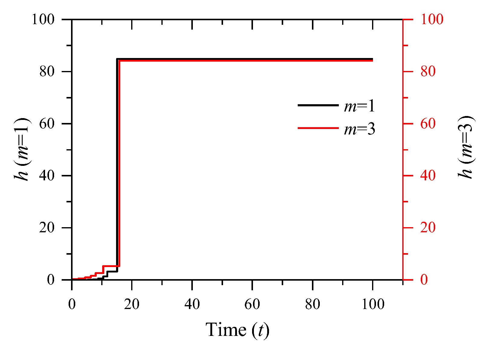
Problem 1 itself is an intrinsically unstable problem. The exact solution of Problem 1 is the exponential function, which soars up rapidly over time and reaches the magnitude of 22,026.47 at $t=10$. This presents a severe challenge to any algorithm with the stringent tolerance $T_l={10}^{-3}\sim {10}^{-6}$ in maximum norm, which means the algorithm should be able to gain at least 8 to 11 exact figures towards the terminal. Table 2 shows the computed results for the problem, and Figure 3 and Figure 4 show the adapted step sizes and error distributions respectively, from which it is seen that proposed algorithm performs very well and all the FE solutions strictly meet the error tolerances.

Problem 2 characterizes the opposite behavior to Problem 1, as its exact solution decays rapidly over time, resulting in a very large final step size as shown in Figure 5. This reflects the adaptivity capability of the proposed algorithm.

Problems 3, 4, and 5 are nonlinear problems and are solved with no difficulties. Problem 6 is a system of nonlinear equations and, although the two solution components comprise a rapidly increased and a rapidly decayed functions, the proposed algorithm solves the problem without difficulties either.

For all the above problems, the proposed algorithm performs satisfactorily and all the computed FE solutions from the reduced elements are able to strictly satisfy the tolerances and hence have made full achievements of the adaptivity objective established in Equation (19).

6.3. A Dynamic Problem

The problem to be solved is a typical single degree-of-freedom problem [22] posed in a second-order ODE form as follows:

$$u^{″}+0.04u^{\prime }+u=\sin (0.2t), u(0)=0, u^{\prime }(0)=1, 0<t\le 256\mathrm{s},$$

(38)

which is typically an equation of motion and physically represents a damped harmonic motion subjected to a dynamic force. The exact solution is shown in Figure 15. By introducing $u_1=u$ and $u_2=u^{\prime }$, the problem can be equivalently transformed to a system of first-order ODEs:

$$u_1^{\prime }=u_2, u_2^{\prime }+0.04u_2+u_1=\sin (0.2t), u_1(0)=0, u_2(0)=1, 0<t\le 256\mathrm{s},$$

(39)

which is solved by using the proposed algorithm with the reduced elements. Please note that, to test the stability of the algorithm for long time domains, a time domain of 256 s has been taken deliberately. The computed results are shown in

Table 8. Results of the dynamic problem (256 s).

Tolerance	Num. of Elements Used	Num. of Element Sizes Altered	Num. of Element Sizes Iterations	Maximum Element Size	Minimum Element Size	True Maximum Element Error Ratio
Tl	Ne	Nalt	Niter	hmax	hmin	${\overline{\mathit{e}}}_{\mathbf{max}}^{\mathit{h}}$
			m = 1
10−3	1542	41	46	0.7835	0.0087	0.90
10−4	4831	88	91	0.3258	0.0290	0.85
10−5	15413	122	125	0.0876	0.0090	0.85
10−6	48539	146	149	0.0268	0.0029	0.85
			m = 3
10−3	162	4	4	2.69	0.87	0.78
10−4	289	5	5	2.03	0.50	0.84
10−5	498	5	6	0.92	0.33	0.83
10−6	887	5	6	0.52	0.20	0.84

and the adapted step sizes and error distributions are shown in Figure 16 and Figure 17, respectively. It is seen that all the FE solutions strictly satisfy the tolerances. It is also observed that the element size has changed at most five times and the number of adaptive iterations is no more than six times.

To access the performance of the reduced element compared with the standard (conventional) elements, the problem has also been solved by using the standard linear and quadratic Galerkin elements (see Section 3) with the same adaptive step-size algorithm using the EEP (Element Energy Projection) [16,17,18,19] super-convergent solution as the error estimator. The computed results are shown in

Table 9. Comparison of performances of different element types (256 s, T_l = 10⁻³).

Element Type	Num. of Elements Used	Num. of Element Sizes Altered	Num. of Element Sizes Iterations	Maximum Element Size	Minimum Element Size	True Maximum Element Error Ratio
	Ne	Nalt	Niter	hmax	hmin	${\overline{\mathit{e}}}_{\mathbf{max}}^{\mathit{h}}$
Standard m = 1	1522	61	69	0.8416	0.0467	15.9
Standard m = 2	319	8	11	3.20	0.50	5.63
Reduced m = 1	1542	41	46	0.7835	0.0087	0.90

and the adapted step sizes and error distributions are shown in Figure 18. It is seen that both standard elements fail to control the error to meet the given tolerance, and that the maximum error ratios are as high as 15.9 for the linear element and 5.63 for the quadratic element. The key reason is that neither of the accuracy ratios reaches two (one for the linear element and four thirds for the quadratic element), and hence neither of them can effectively provide satisfactory results.

7. Conclusions

A new type of finite element model, called the reduced element, for adaptive analysis of the first-order IVPs in maximum norm is presented in this paper. The main idea is simply to decompose the conventional FE solutions into two parts, i.e., a reduced element solution serving as the final solution and an error term serving as a built-in pointwise error estimator. A complete adaptivity algorithm is developed based on the reduced element with reliable error control and effective step-size adjustment. Mathematical analysis and numerical results show that, for both linear and nonlinear IVPs of both single and system of ODEs, the proposed approach can produce solutions that satisfy the preset error tolerance in a satisfactory and reliable fashion.

References

1. Henrici, P. Discrete Variable Methods in Ordinary Differential Equations; Wiley: New York, NY, USA, 1962. [Google Scholar]
2. Ceschino, F.; Kuntzmann, J. Numerical Solution of Initial Value Problems; Prentice-Hall: Englewood Cliffs, NJ, USA, 1966. [Google Scholar]
3. Gear, C.W. Numerical Initial Value Problems in Ordinary Differential Equations; Prentice-Hall: Englewood Cliffs, NJ, USA, 1971. [Google Scholar]
4. Strang, G.; Fix, G.J. An Analysis of the Finite Element Method; Prentice-Hall: New York, NY, USA, 1973. [Google Scholar]
5. Keller, H.B. Numerical Solution of Two Point Boundary Value Problems; Society for Industrial and Applied Mathematics: Philadelphia, PA, USA, 1976. [Google Scholar]
6. Fletcher, C. Computational Galerkin Methods; Springer: New York, NY, USA, 1984. [Google Scholar]
7. Butcher, J.C. Numerical Methods of Ordinary Differential Equations; Wiley: New York, NY, USA, 2016. [Google Scholar]
8. Dormand, J.R.; Price, P.J. A family of embedded Runge–Kutta formulae. J. Comput. Appl. Math. 1980, 6, 19–26. [Google Scholar] [CrossRef]
9. Higham, D.J. Robust defect control with Runge–Kutta methods schemes. SIAM J. Numer. Anal. 1989, 26, 1175–1183. [Google Scholar] [CrossRef]
10. Calvo, M.; Higham, D.J.; Montijano, J.I.; Rández, L. Global error estimation with adaptive explicit Runge–Kutta methods. IMA J. Numer. Anal. 1996, 16, 47–63. [Google Scholar] [CrossRef]
11. William, J.L. Galerkin methods for two-point boundary value problems for first-order systems. SIAM J. Numer. Anal. 1983, 20, 161–171. [Google Scholar]
12. Delfour, M.; Hager, W.; Trochu, F. Discontinuous Galerkin methods for ordinary differential equations. Math. Comp. 1981, 36, 453–473. [Google Scholar] [CrossRef]
13. Hulme, B.L. One-step piecewise polynomial Galerkin methods for initial value problem. Math. Comput. 1972, 4, 415–426. [Google Scholar] [CrossRef]
14. Douglas, J.; Dupont, T. Galerkin approximations for the two point boundary problems using continuous, piecewise polynomial spaces. Numer. Math. 1974, 22, 99–109. [Google Scholar] [CrossRef]
15. Douglas, J.; Dupont, T. Galerkin methods for parabolic equations. SIAM J. Numer. Anal. 1970, 7, 575–626. [Google Scholar] [CrossRef]
16. Xiao, C. Adaptive FEM Analysis for Systems of First-Order ODEs Based on EEP Super-Convergent Method. Ph.D. Thesis, Tsinghua University, Beijing, China, 2009. (In Chinese). [Google Scholar]
17. Yuan, Q. A Family of High Performance Galerkin Elements and Adaptive-Stepped Analysis of Motion Equation. Ph.D. Thesis, Tsinghua University, Beijing, China, 2023. (In Chinese). [Google Scholar]
18. Yuan, S.; Xing, Q.; Wang, X.; Ye, K. Self-adaptive strategy for one-dimensional FEM based on EEP method with optional superconvergence order. Appl. Math. Mech. 2008, 29, 591–602. [Google Scholar] [CrossRef]
19. Yuan, S.; Du, Y.; Xing, Q.; Ye, K.S. Self-adaptive one-dimensional nonlinear finite element method based on element energy projection method. Appl. Math. Mech. 2014, 35, 1223–1232. [Google Scholar] [CrossRef]
20. Yuan, S.; Yuan, Q. Condensed Galerkin element of degree m for first-order initial-value problem with O(h2m+2) super-convergent nodal solutions. Appl. Math. Mech. 2022, 43, 603–614. [Google Scholar] [CrossRef]
21. De Boor, C.; Weiss, R. Solveblock: A package for solving almost block diagonal linear system. ACM Trans. Math. Softw. 1980, 1, 80–87. [Google Scholar] [CrossRef]
22. Clough, R.; Penzien, J. Dynamics of Structures; McGraw-Hill: New York, NY, USA, 1993. [Google Scholar]
Figure 1. Structure of the reduced linear element: linear element with quadratic nodal values.
Applsci 14 07264 g001
Figure 2. An illustrative sample of one element solution (h = 3.5). For the reduced linear solution u R h , the true error u u R h is very closely estimated by the calculated error u Q h u R h with higher order nodal errors.
Applsci 14 07264 g002
Figure 3. The step-size distribution of Problem 1 (Tl = 10−5).
Applsci 14 07264 g003
Figure 4. The error ratio variation of Problem 1 (Tl = 10−5).
Applsci 14 07264 g004
Figure 5. The step-size distribution of Problem 2 (Tl = 10−5).
Applsci 14 07264 g005
Figure 6. The error ratio variation of Problem 2 (Tl = 10−5).
Applsci 14 07264 g006
Figure 7. The step-size distribution of Problem 3 (Tl = 10−5).
Applsci 14 07264 g007
Figure 8. The error ratio variation of Problem 3 (Tl = 10−5).
Applsci 14 07264 g008
Figure 9. The step-size distributions of Problem 4 (Tl = 10−5).
Applsci 14 07264 g009
Figure 10. The error ratio variations of Problem 4 (Tl = 10−5).
Applsci 14 07264 g010
Figure 11. The step-size distributions of Problem 5 (Tl = 10−5).
Applsci 14 07264 g011
Figure 12. The error ratio variations of Problem 5 (Tl = 10−5).
Applsci 14 07264 g012
Figure 13. The step-size distributions of Problem 6 (Tl = 10−5).
Applsci 14 07264 g013
Figure 14. The error ratio variations of Problem 6 (Tl = 10−5).
Applsci 14 07264 g014
Figure 15. The exact solution of the dynamic problem.
Applsci 14 07264 g015
Figure 16. The step-size distribution of the dynamic problem (m = 3, Tl = 10−3).
Applsci 14 07264 g016
Figure 17. The error ratio variation of the dynamic problem (m = 3, Tl = 10−3).
Applsci 14 07264 g017
Figure 18. The error ratio variations of the dynamic problem by standard linear and quadratic elements (Tl = 10−3).
Applsci 14 07264 g018