Prediction of Structural Fracture Distribution and Analysis of Controlling Factors in a Passive Continental Margin Basin—An Example of a Clastic Reservoir in Basin A, South America

Abstract

Structural fracture distribution is essential in oil and gas transportation and development in passive continental margin basins. In this paper, taking as an example the clastic reservoirs in the A-Basin, a passive continental margin in northeastern South America, the paleotectonic stress field of the Late Cretaceous Maastrichtian formation in Basin A was numerically simulated by finite element technique through the integrated interpretation of seismic total data, logging data and core data, and the distribution of tectonic fractures was later predicted based on rock fracture criterion. The results of the study show that: (1) The distribution of tectonic stress and fractures during the Late Cretaceous Maastrichtian formation of Basin A is affected by the fracture zone, mechanical properties of rocks and tectonic stress, regions with extensive fracture development are susceptible to stress concentrations, resulting in significant stress gradients. (2) The development of structural fractures in the study area was predicted using the Griffiths criterion, and the tensile rupture coefficient T was introduced to quantitatively characterise the intensity of fracture development, with larger values reflecting a higher degree of fracture development. The well-developed and relatively well-developed fractures are mainly located in the fracture zones and the interior of submarine fans. (3) Fracture zones and sedimentary phases mainly control structural fractures in Basin A; within 5 km outside the fracture zones, the development of fractures is controlled by the fracture zones, beyond which the regional tectonic stress field controls them; inside the sedimentary fan, the development of fractures is controlled by the sedimentary subphase, which decreases in the order of the upper fan, the middle fan, and the lower fan; inside the subphase, they are controlled by the regional tectonic stress field, and the fractures show the increasing trend in the direction of NW-NE.

1. Introduction

Deep water in the passive continental margin basin has been the focus of global oil and gas exploration over the last decade [1,2,3]. In Basin A, the marine hydrocarbon source rocks in the drift period are widely distributed and of good quality, with abundant oil sources. The basin mainly develops Cretaceous-Tertiary sandstone reservoirs and some carbonate reservoirs [4]. It is found that the hydrocarbon source rocks near the target reservoir are immature, and the vertical distance between the target layer and the mature hydrocarbon source rocks is more than 1 km due to the tectonic flatness of the period of drifting and the limited development of fracture. Nevertheless, research has discovered the presence of steep faults that, along with their corresponding fracture systems, can serve as vertical channels for the transportation of hydrocarbons [5]. Therefore, studying the distribution characteristics of reservoir structural fractures and the main controlling factors is of great theoretical and practical significance for the rational development of passive continental margin basin.

Currently, the mainstream fracture prediction and modelling methods include the binary, fractal and dimensional, seismic attribute analysis, maximum curvature method, and numerical simulation of tectonic stress field [6]. The binary method integrates the fracturing method with the energy method to predict reservoir fractures. It develops a mathematical model to quantitatively predict fractures by analysing the relationship between single-well values, energy values, and fracture densities [7,8]. However, it does not consider the impact of the stress field on structural fractures, resulting in the ability only to determine the distribution of fracture line density. Fractal theory suggests that fractures formed by rock rupture have fractal characteristics [9]. The fractal dimension can quantitatively characterise the degree of reservoir fracture development. Guanghui Wu et al. [10] By studying Tarim carbonate reservoir fractures, it is concluded that the degree of reservoir fracture development is positively correlated with the fractal dimension, and the greater the fracture density, the greater the fractal dimension. Still, this method is only used in areas with a high degree of fracture development and is limited by the accuracy of the tectonic interpretation of seismic data.

Geophysical methods can indirectly reflect fractures’ development through changes in fractured reservoirs’ physical characteristics. Fractures can be detected by varying seismic wave propagation time, velocity, amplitude, and frequency at different azimuths in an anisotropic medium. Seismic techniques for fractured reservoir prediction include transverse wave splitting, multi-wave multi-component detection, seismic attribute analysis, etc. [11] Dong Chunmei et al. [12] summarised the fracture indication parameters and fracture identification methods based on conventional logging. Weiguang Hu [13] used the coherent body technique to predict the distribution of fracture development zones and fractures in the study area. Xiaomei Liu et al. [14] combined multivariate statistical analysis, seismic attributes, and adaptive fuzzy neural networks to comprehensively predict fractured reservoir distribution concerning reservoir cohomogeneity and anisotropy characteristics. Wen Gu et al. [15] post-stack seismic attribute analysis techniques are utilised to forecast fractures in fractured reservoirs, and a multi-attribute approach has been developed for predicting reservoir fractures. While the 3D seismic data encompass a broad scope of regions, their effectiveness is constrained by the quality and precision of the seismic measurements. Consequently, they can solely identify fracture development zones that are of significant scales and sizes. The fracture prediction method based on the tectonic stress field relies on geomechanical theory [14]. It begins by examining the connection between the tectonic stress field and the mechanical properties of the reservoir rock. Through experimental and theoretical derivation, a mechanical model of stress–strain and the mechanical parameters of the reservoir rock is established, assuming a preferred rupture criterion. Subsequently, the stress field and fracture rupture coefficients are determined. This method has gained popularity recently and has been successfully implemented in various locations. [16,17,18,19,20,21,22,23,24,25,26,27,28,29].

The Late Cretaceous Maastrichtian Formation in Basin A is rich in oil and gas resources, and the oil and gas are transported through fractures. Structural fractures are essential factors affecting reservoir quality and well capacity. However, the structural fracture development and distribution pattern of the Late Cretaceous Maastrichtian Formation in this area still needs to be clarified, and the influencing factors are unknown, which seriously restricts the efficient development of oil and gas resources.

In this paper, by predicting the reservoir fracture characteristics and development and distribution patterns in the study area, the main controlling factors are identified to provide a basis and reference for optimising the reservoir development plan.

2. Materials and Methods

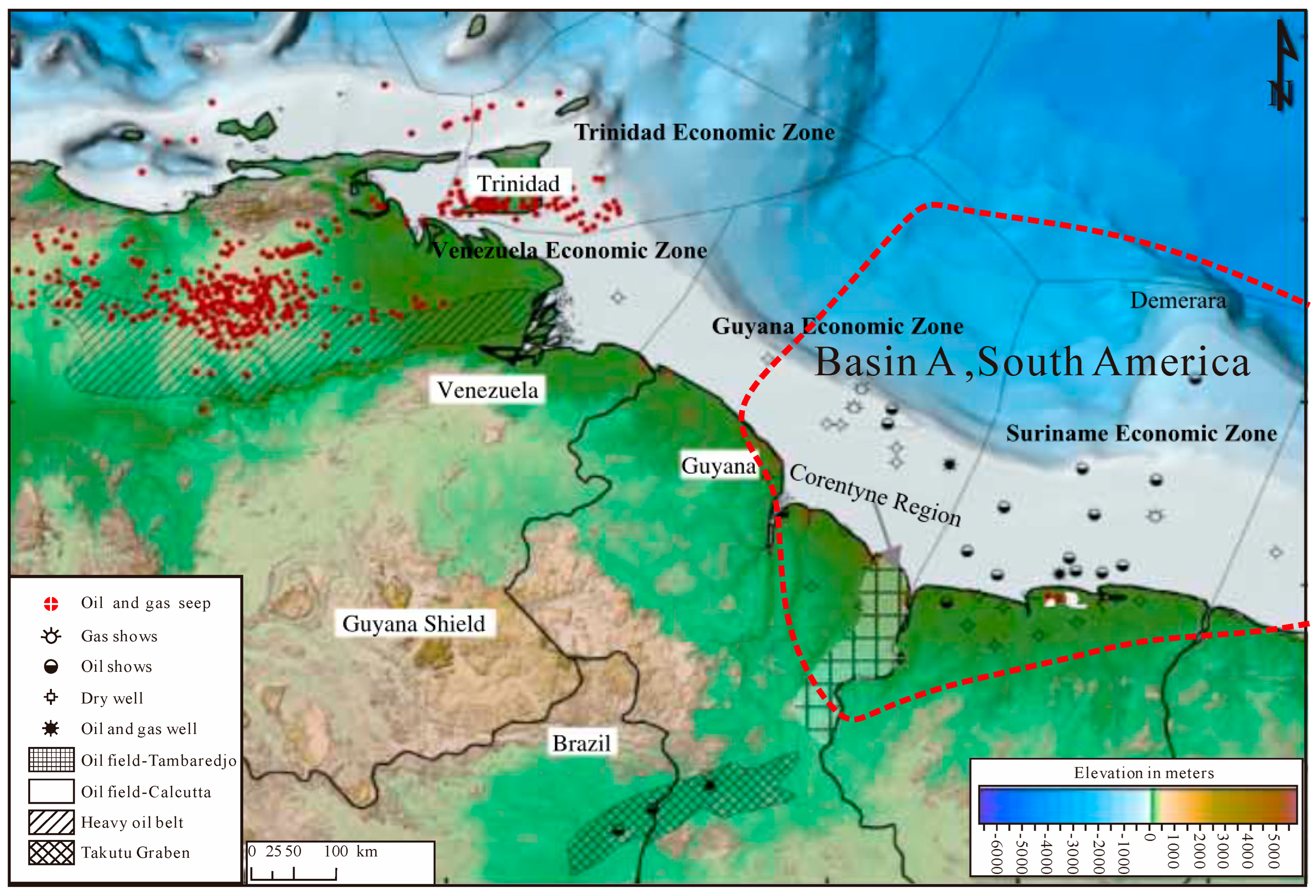
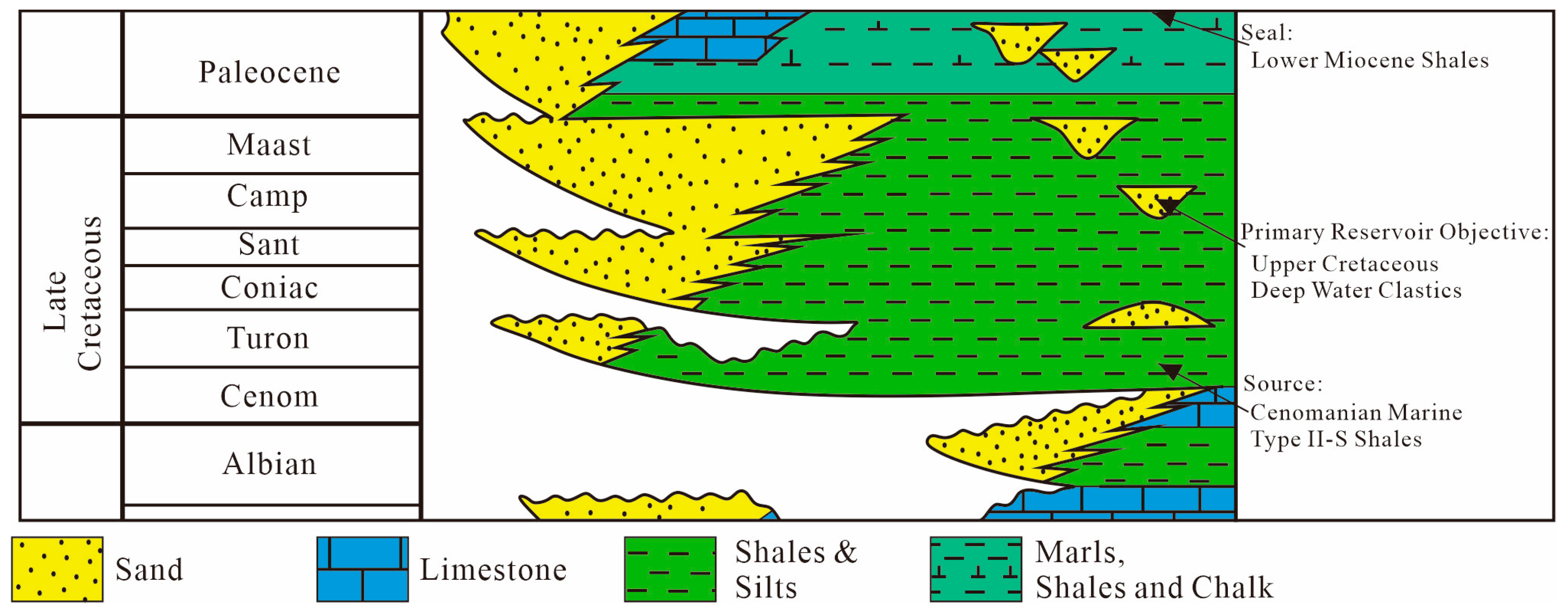
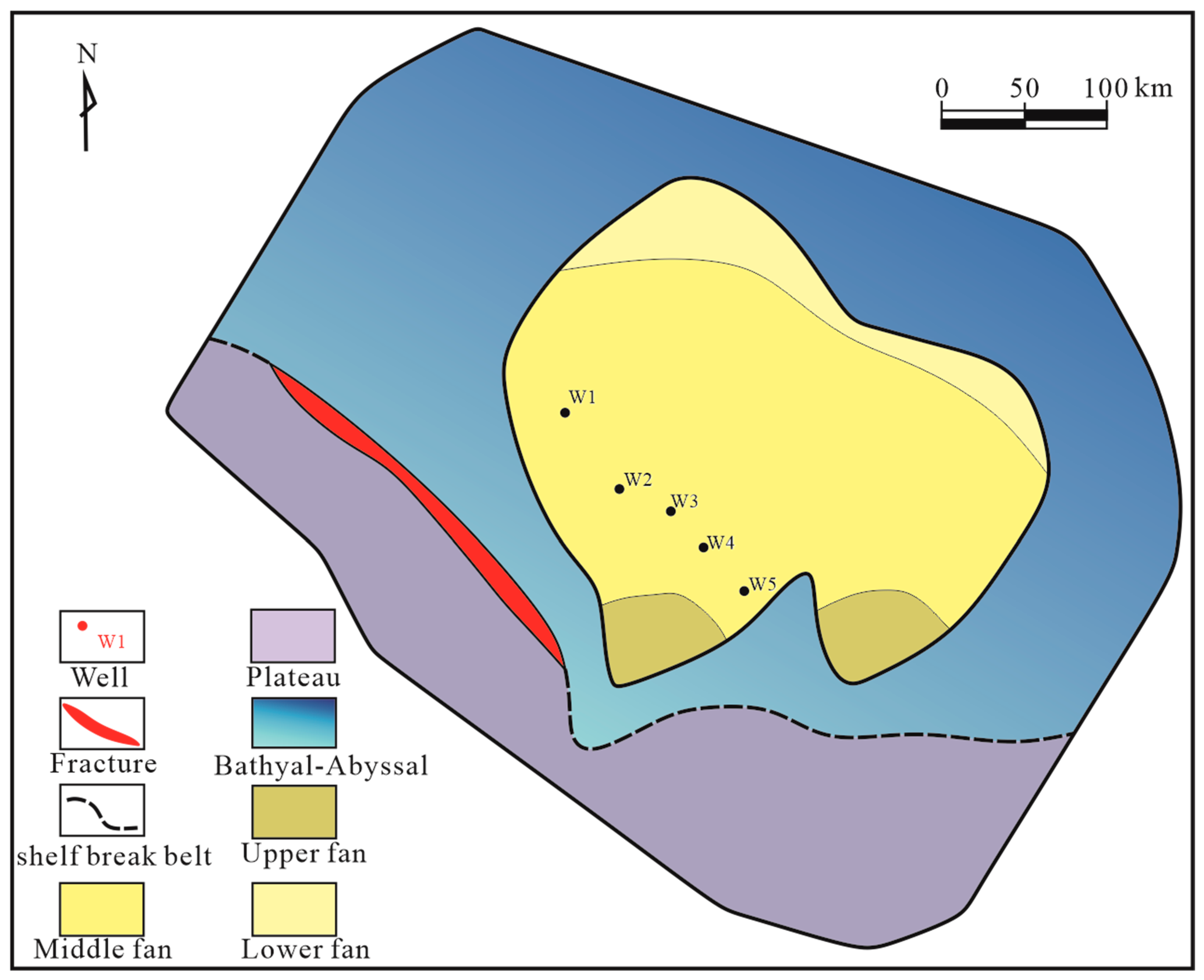
2.1. Regional Geological Setting

Basin A is a passive continental margin basin formed by the separation of the South American and African plates as a result of the rifting of the Gondwana continent (Figure 1); it mainly experienced two stages of evolution, the Jurassic-Cretaceous to Aptian rift and the passive marginal stage since the Albian, and developed the NW-SE Early Cretaceous high-angle tensile fractures parallel to the shelf, the stratigraphy of the basin is relatively continuous, and mud shale, deep-water turbidite sandstone, carbonate rocks, etc., are well developed (Figure 2) [30].

The overall seismic pattern of the basin is a typical passive margin that evolves upward during the sag and thermal cooling phase from a ramp to prograding geometries. These geometries are controlled mainly by accommodation created by eustacy and extensional tectonics with strike–slip influence from the Guyana Transform (Figure 3). These geometries are mainly controlled by regulating extensional structures affected by subduction and strike–slip [31]. Based on the tectonic interpretation, three stages of tectonic development can be identified: (i) Triassic-Jurassic Rift Phase. (ii) Lower Cretaceous Strike Slip Influenced Passive Margin Phase. (iii) Upper Cretaceous-Recent Passive Margin Phase [32].

The Triassic–Jurassic Rift Phase is characterized by the active development of half grabens and synrift terrestrial facies related to the initial stages of the extensional grains related to the proto Central Atlantic opening (Figure 3A). The second phase is related to an extended flooding of the Guyana Craton and the development of a ramp setting dominated by carbonates during the Lower Cretaceous. Synchronally, the development of a NW-SE transform controlled the subsequent opening of the proto–South Atlantic and the separation of the Deremara Rise from the Guinea Plateau. The transform activity created a series of structured inverted features until the Upper Cretaceous (Figure 3B). The third stage is a typical passive margin, Africa drifted away from South America, which formed the main extensional geologic regime in the Guyana Basin and caused a general collapse of the unstable shelf edge and slope (Figure 3C). This predominantly transcurrent movement occurred mostly from the Albian to the Eocene, but is still active at present

The Late Cretaceous Maastrichtian Formation possesses good physical characteristics, abundant drilling and seismic data, and lacks fracture zones. Through the observation and statistics of the core, it is found that high-angle structural tension fractures develop, and oil and gas are shown in the fractures. Through the examination of the logging data, it is evident that the natural gamma curve displays funnel, bell, low-amplitude micromoth, and box-funnel composite shapes. The sedimentary phases progress from west to east, consisting of the shallow tableland phase, submarine fan phase, and deep-sea in-situ deposition. Within the sedimentary submarine fan phase are three subphases: the upper fan, middle fan, and lower fan subphases (Figure 4). The lithologies consist of sandstone and siltstone, including silt, sandy siltstone, sandy marl, marl, mudstone, and sandy mudstone.

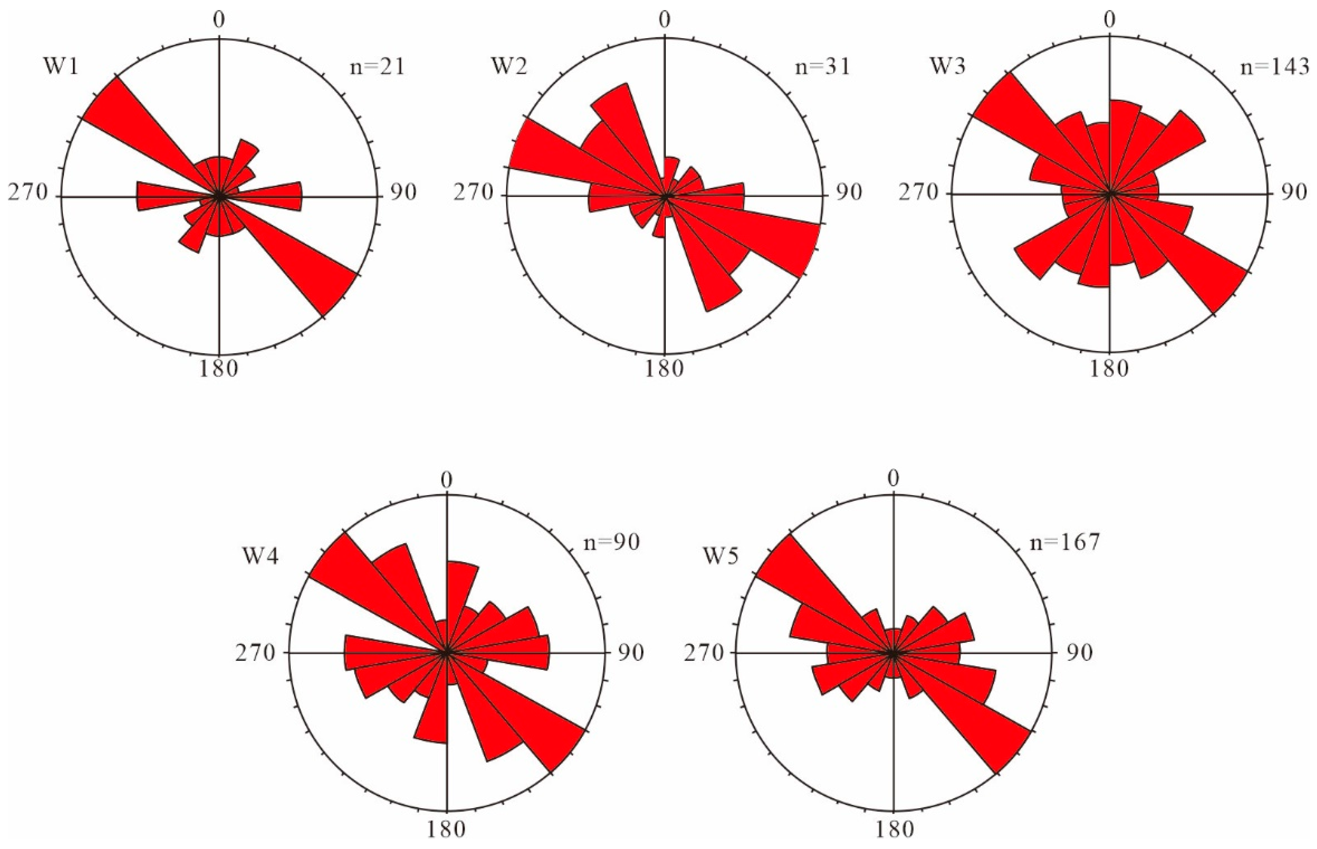
2.2. Structural Fracture Characteristics

452 structural fractures were measured and collected in five logging cores in Basin A. The characteristics of these fractures indicate that they are mainly high-angle tension fractures formed under the action of a tectonic stress field [33] (Figure 5). Usually, tensile fractures are characterised by high-angle fractures in the core, which are curved, have short extension distances, and are unstable (Figure 5e) [34,35]. The edges of the fractures show jagged edges, and the fracture surfaces are rough and uneven without scratch. Fracture grouping is not apparent, with a certain degree of openness, but is often half-filled by minerals such as square zeolite and calcite (Figure 5b). Tension fractures sometimes constitute serrated tracking tension joints, monoclinic or conjugate geese-row tension joints, etc. Observations of the fractures in the core in Basin A revealed that they have dendritic bifurcation (Figure 5c). Its small nodules are not oriented; amygdaloidal and amygdaloidal nodules are elliptical, with inconspicuous rhombic angles (Figure 5d). Fluorescent reflections are observed in all fractures (Figure 5f), proving it has oil and gas filling.

Fracture statistics from the drilling imaging logs in Basin A indicate that high-angle tension fractures dominate natural fractures (Figure 5a). The fracture tendency of the W1 well is mainly NEE and NNW, the dip angle 40~80° is dominant, and the fracture strike is NWW-SEE dominant, 120~140°. The fracture tendency of the W2 well is SEE dominant, 100~120°. The fracture tendency of the W3 well is SNE dominant, 120~140° dominant. The fracture tendency of the W4 well is SEE dominant, 120~140° dominant. The fracture tendency of the W5 well is mainly NNE, the fracture strike is NWW-SEE, the fracture strike is mainly 120~140°, and the dip angle is mainly 50~60°. The dominant fractures are distributed primarily in the direction of NNW~SSE (Figure 6).

According to classical theories in Structural Geology [36] and characteristics of natural fractures in basin A, NNW~SSE-trending tensile fractures were formed under the passive margin phase paleotectonic stress field. The types and orientations of structural fractures deduced based on stress analysis in Basin A can be validated from well and drill core data.

2.3. Method for Numerical Simulation of Tectonic Stress Field

Based on logging data, including standard logging information (i.e., gamma, sonic, density, and resistivity) from five exploratory wells, lithologic data, and stratigraphic layering, Seismic data are 2D paleoseismic interpretations published by Yang and Escalona [30]; Establishment of a reliable tectonic model (taking into account variations in stratigraphic thickness and the distribution of fractures) using mathematical and mechanical methods, using a map of sedimentary phases and stress data from a limited number of measurement points [37,38,39], Designing a rational finite element partitioning scheme [39,40,41,42], The stress field within the formation during the critical tectonic evolution period was predicted using Ansys software (v. 19.0) under different directional boundary stress loads. Eventually, the coupling law between the distribution of tectonic stress and the distribution law of geological tectonic traces or oil and gas resources is analysed, and the formation and enrichment law is studied, as well as the prediction of oil and gas reservoirs.

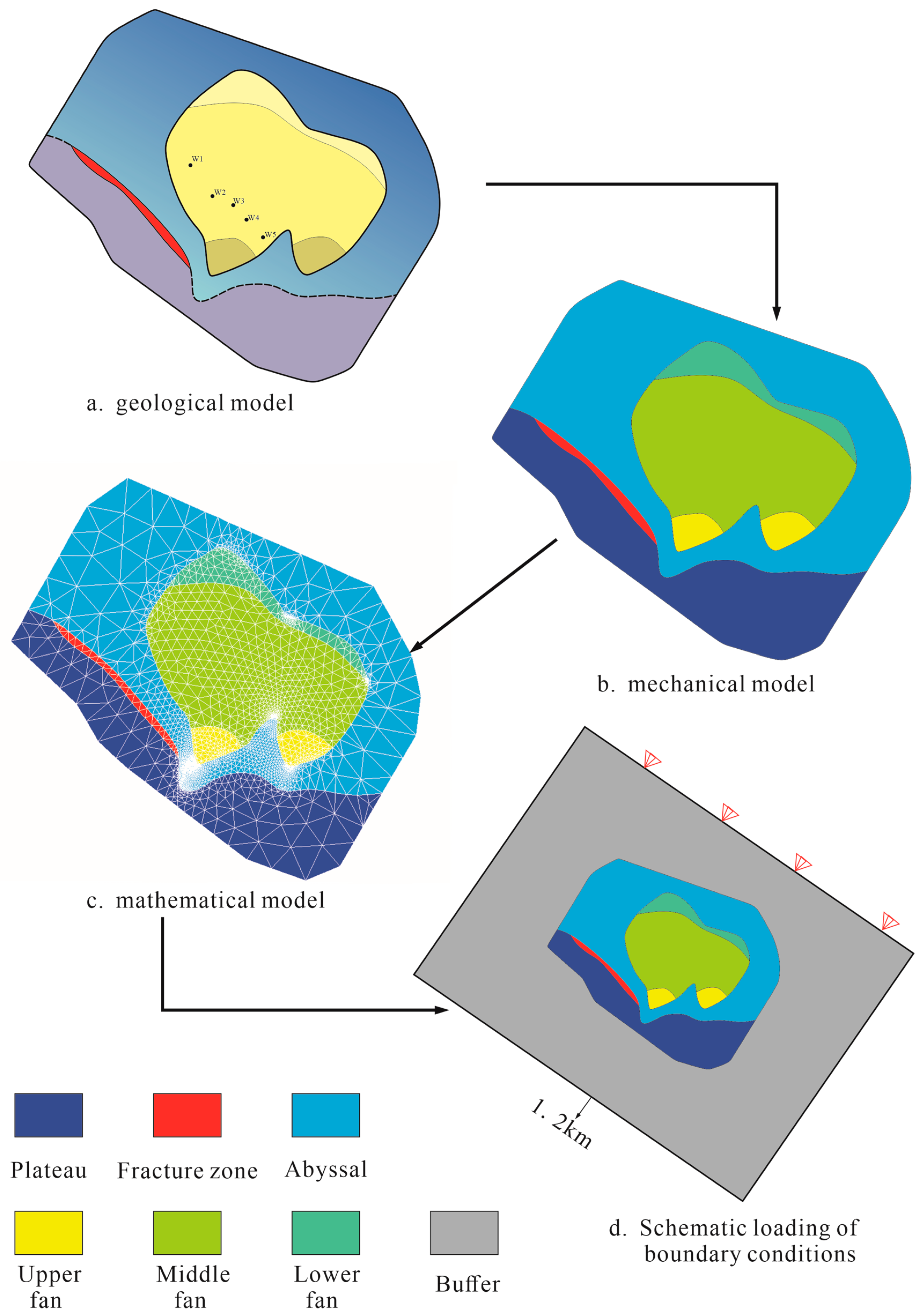
2.3.1. Geological Model

The geometry of the initial model is based on the sedimentary phase plan and tectonic map. The mechanical data of the rocks in different sedimentary phases are calculated and counted, and the parameters are projected according to the type of sedimentary phase to differentiate the values of the petrophysical parameters of the different kinds of sedimentary phases. Secondly, the average values of petrophysical parameters of different sedimentary phases are obtained according to the projection map. Finally, the phase types are simplified into three modules: shelf slope folding zone, abyssal, and sedimentary fan, combined with the tectonic map (Figure 7a). The average values of the parameters obtained are assigned to these three modules. Then, according to the actual geological condition of the stratum in Basin A, the model is divided into finite element modelling.

2.3.2. Mechanical Model

In the finite element modelling process, material properties are assigned to these units to build the geological model (Figure 7a). To transform the geologic model into a mechanical model that can be used for finite element numerical simulation, this paper determines the rock mechanical parameters such as Young’s modulus of elasticity, Poisson’s ratio, and rock density of different geologic units for the Maastrichtian Formation mechanical parameters from the inversion of the seismic wave data and the analysis and computation of the five well logging data. Where rock density can be derived from density logging curves, Young’s modulus of elasticity Equation (1) and Poisson’s ratio Equation (2) can be calculated using logging data [43]:

$$E_d={\displaystyle \frac{{\rho }_b}{{∆t}_s^2}}\times {\displaystyle \frac{3{∆t}_s^2-4{∆t}_p^2}{{∆t}_s^2-{∆t}_p^2}}$$

(1)

$${\mu }_d={\displaystyle \frac{{∆t}_s^2-2{∆t}_p^2}{2\left({∆t}_s^2-{∆t}_p^2\right)}}$$

(2)

$E_d$ is Young’s modulus of elasticity (GPa); ${\mu }_d$ is Poisson’s ratio; ${\rho }_b$ is the rock density (kg/m³); ${∆t}_p$ and ${∆t}_s$ is Longitudinal and transverse time differences (μs/m).

Because the mechanical properties of the fracture zone are difficult to determine, it is set as a weak zone in the model [44,45]. In this analysis, Young’s modulus, angle of internal friction, rock cohesion, and tensile strength parameters for the weak zone were defined as 70% of the mean value of the Maastrichtian Formation parameters. The Poisson’s ratio in the fracture zone is generally large, with differences ranging from 0.02 to 0.10. The value of the buffer zone is usually selected as the average value of Young’s modulus and Poisson’s ratio in the study area (except the fracture zone) [46]; the rock mechanical parameters of the fracture zone should be differentiated according to the scale of the fracture, Young’s modulus is generally selected as 50~70% of the surrounding rock; the Poisson’s ratio of the fracture area is larger than that of the normal depositional area, and the difference between the two is usually between 0.02~0.1 [47]. After the rock mechanical parameters of different geologic units are determined (

Table 1. Rock mechanical parameters of the Maastrichtian Formation geologic unit in Basin A.

Rock Mechanics Parameters	Mechanical Unit
	Abyssal	Upper Fan	Middle Fan	Lower Fan	Plateau
Young’s modulus of elasticity/Gpa	16.80	17.17	19.62	24.75	27.50
Poisson’s ratio	0.317	0.296	0.312	0.262	0.248
tensile strength/Mpa	11.25	11.09	12.08	12.65	13.00

), corresponding rock mechanical parameters are assigned to the geologic units, and the mechanical model is established (Figure 7b).

2.3.3. Mathematical Model

The entire model is meshed using triangular cells (Figure 7c). Element size affects the resolution of prediction results. Smaller element sizes usually produce better results; However, at the same time, it requires better hardware equipment and a longer computation time. Based on the model area, this study used a level 1 (ranging from 1–10 in ANASY software (v. 19.0), with 1 being the best) meshing resolution. After meshing, there are 7108 nodes in the model.

2.3.4. Boundary Conditions

To minimise boundary effects, the study area is nested within a rectangular buffer in this paper (Figure 7d), utilising the principle of conservation of equilibrium profiles [48,49] and Selecting profiles perpendicular to the regional tectonic line. Then, with the help of 2Dmove software (v. 2018), the expansion amount of the basin was obtained by performing the compaction and de-compaction correction-breakage elimination-layer flattening process of the tectonic layers in the present-day profile using the equilibrium profiling technique [50]. Finally, the results show that the length of this present-day profile is 55.4 km, and the size of the recovered profile is 54.2 km, with an elongation of 1.2 km in the NE-SW direction.

2.4. Method for Structural Fracture Prediction

The core fracture data study shows that most fracture types in the formations of the study area are tensile fractures, which are essential for petroleum exploration and development.

The principal fracture criteria for rocks include the Drucker–Prager criterion, the Unified Strength Theory, the Griffith criterion, and the Hoek–Brown criterion [51]. Shear fracture and tensile fracture are the main types of rock fracture due to tectonic stresses. The Morcuran shear fracture criterion describes shear fractures, while the Griffiths fracture criterion forecasts tensile fractures. The tectonic morphology of the Maastrichtian Formation in Basin A is shaped by the stretching forces, so this paper predicts the occurrence of structural fractures using Griffith’s criterion theory.

2.4.1. Griffith Criterion

The Griffith criterion is generally used to determine the degree of rupture for tensile rupture of brittle materials. In 1921, Griffith argued that the damage of brittle materials is controlled by a wide range of randomly distributed microfractures in the material, which are prevalent in structural surfaces, sedimentation, etc., in rocks. When the rock is subjected to external forces, stress concentration occurs at the tips of microfractures conducive to rupture, leading to fracture expansion to form tensile fractures.

The mathematical expression for the three-dimensional Griffith criterion is:

$$\sigma 1+\sigma 3\ge 0, (\sigma 1-\sigma 3)2 + (\sigma 2-\sigma 3)2 + 24{\sigma }_{\mathrm{T}}(\sigma 1+\sigma 2+\sigma 3)= 0$$

(3)

$$\sigma 1+3\sigma 3<0, \sigma 3+{\sigma }_{\mathrm{T}}=0$$

(4)

$\sigma 1$, $\sigma 3$ and $\sigma$2 are the maximum, minimum, and intermediate principal stresses, respectively. In contrast, extrusions are positive, tensions are negative, ${\sigma }_{\mathrm{T}}$ is the tensile stress on the rupture surface.

2.4.2. Calculation of Rupture Factor

To determine the development of tensile fractures in the stratigraphy of the study area, a tensile rupture coefficient T was introduced with the expression [52]:

$$\mathrm{T} = {\sigma }_{\mathrm{T}}/{\sigma }_{\mathrm{t}}$$

(5)

${\sigma }_{\mathrm{t}}$ is the rock’s tensile strength, which can be calculated. ${\sigma }_{\mathrm{T}}$ is the equivalent tensile stress of the rock, and the distribution of the maximum principal stress and the minimum principal stress obtained from the numerical calculation of the stress field simulation can be calculated by Equations (4) and (5).

According to the size of the T-value, the rupture of the rock can be judged accordingly. If T ≥ 1, the rock rupture occurs, and the larger the T-value, the more fractures are developed in the rock.

3. Results

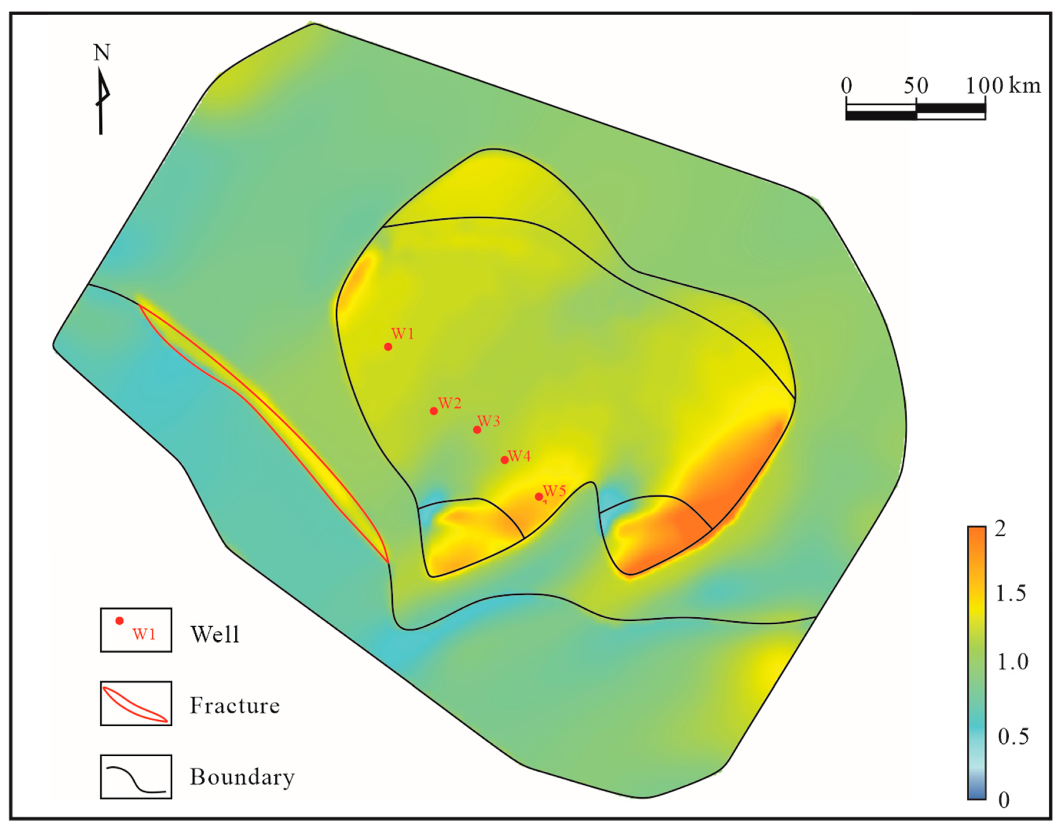
3.1. Results of Stress Modelling

The maximum principal stress simulation results show (Figure 8a) that the maximum principal stress of the Late Cretaceous Maastrichtian Formation is centrally distributed in the range of 1.5–4 Mpa, with a gradual decrease in the stress value from the NE direction to the SW direction, and a smaller range of change in the overall stress value of about 2.5 Mpa. Overall, there is a specific correlation with the sedimentary phase zone, and the stress contours form a NE-SW-trending strip distribution. In addition, the stress gradient of this low-value zone is closely related to the fracture strength, and the greater the fracture strength, the greater the maximum principal stress gradient.

The minimum horizontal principal stress simulation results show (Figure 8b) that the minimum principal stress of the Late Cretaceous Maastrichtian Formation is centrally distributed between 24–33 MPa, with a gradual increase in stress values in the east-direction from north-west to south-east and a small range of variation in the overall stress values of about 9 MPa. Like the factors influencing the maximum horizontal principal stress distribution, fractures and sedimentary phases also control the minimum horizontal principal stress, and the stress contours form a NE-SW trending strip-like distribution. In the southern part of the study area, the stress values are relatively large; in the northern part, the stress values are relatively small. The fracture area exhibits low-stress values, while high-stress values are concentrated at the termination point of the fracture.

3.2. Results of Fracture Prediction

Maastrichtian Formation rupture coefficient for Basin A calculated from tectonic stress field simulation results and equations (Figure 9). Fracture prediction results show that the integrated rupture coefficient value of Maastrichtian Formation in Basin A is mainly distributed between 0.4–2.0, and the distribution trend is greatly influenced by the distribution of fractures and sedimentary phases; among them, the rupture coefficients of fracture zones in the fracture zone area are all over 1.4, and the rupture coefficients of fracture zones of the abyssal sea and the slope folding zones of the shelf are smaller than that of the interior of the sedimentary fan as a whole. Still, the whole trend shows an increasing trend toward NW-SE. Using the fracture coefficient as a metric, areas of better Maastrichtian Formation fracture development and relatively better fracture development in Basin A were predicted.

4. Discussion

4.1. Evaluation of Fracture Prediction Results

Possible limitations and pitfalls in the application of finite element modelling, including:

(i) The rock assemblage in Basin A is laterally highly variable, with different rock types exhibiting different rock mechanical properties, creating non-homogeneity. However, within the finite element model, Basin A is divided into facets that are treated as nearly homogeneous. This situation is almost impossible to avoid unless the focusing region is reduced to a small area, such as drilling profiles [53].

(ii) The finite element model uses regional boundary conditions that ignore specific localised stresses in some regions.

Despite these limitations, the results of structural fracture prediction were analysed. Maastrichtian Formation densities were calculated over five wells in Basin A. The relationship between Maastrichtian Formation fracture densities and fracture coefficients in Basin A is shown in (Figure 10):

$$D_f=0.3947\mathrm{x}+0.7343 ({\mathrm{R}}^2=0.9712)$$

(6)

$D_f$ is the fracture density, R is the correlation coefficient.

Fracture line density and rupture coefficient during the Maastrichtian Formation in Basin A are linearly correlated, and the higher R-value indicates that the predictions are in good agreement with the actual situation, although the numerical simulation is flawed.

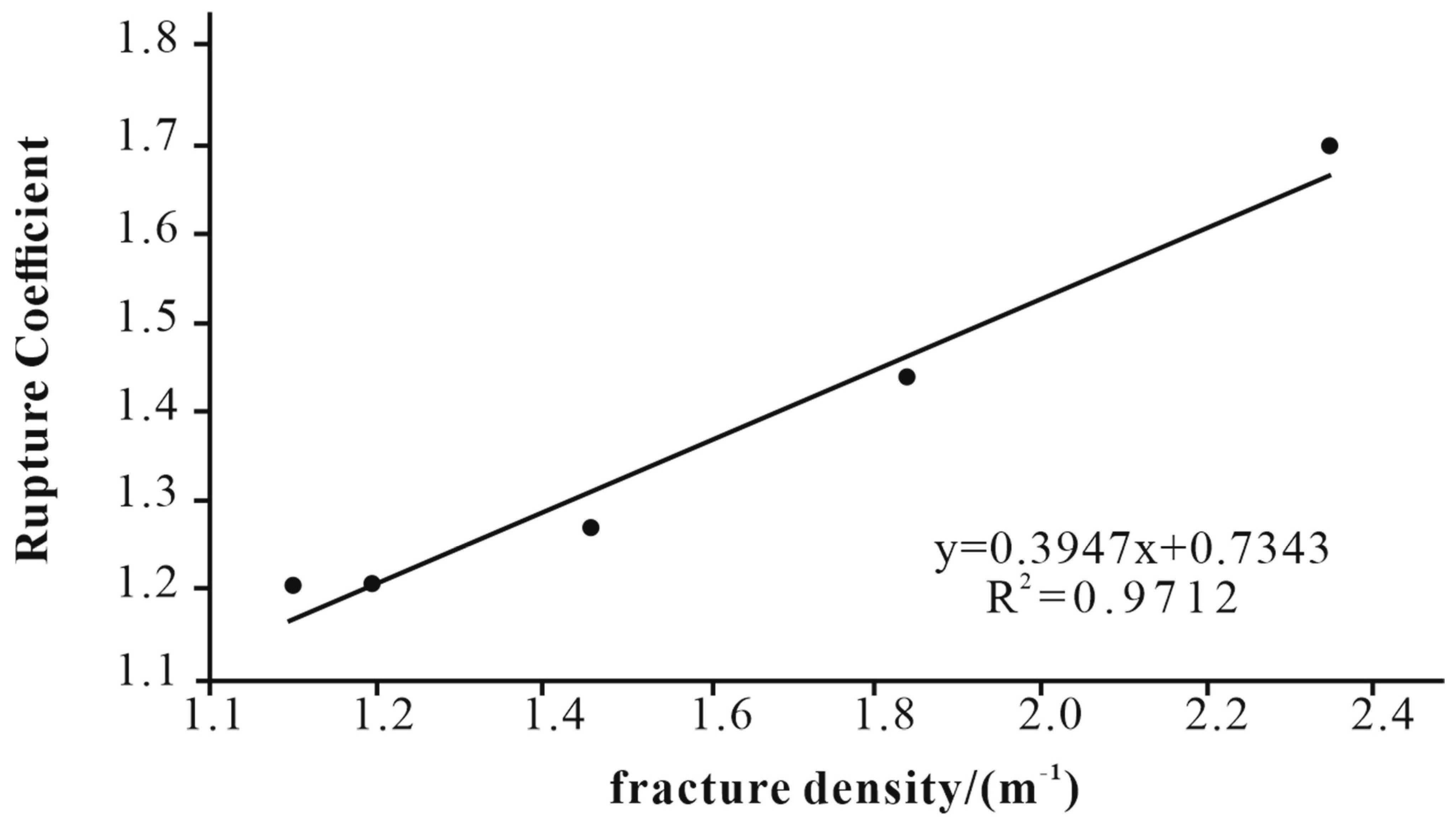
4.2. Controlling Factors for Structural Fractures

Factors affecting the development and distribution of structural fractures are mainly categorised into tectonic and non-tectonic factors [53,54,55,56]. Tectonic activity, sedimentary phases, etc., mainly control the Maastrichtian’s structural fractures in basin A.

4.2.1. Relationship between Fracture Zone and Fracture

In general, structural fractures are more likely to be accompanied by fracturing and folding activity [44]; this paper mainly applies the rupture coefficient of structural fractures to study structural fracture development and distribution law.

Three profiles were selected perpendicular to the rupture on the Maastrichtian Formation rupture coefficient map of Basin A. Then, the fracture coefficient is read at a certain distance on the selected profile. It should be noted that the three chosen profiles are located in areas with few fractures and relatively simple geological structures, so the influence of other factors (submarine fan) can be excluded. Thus, the development and distribution of structural fractures in these areas are mainly influenced and controlled by the fracture zones, and the results obtained can more genuinely reflect the correlation between the rupture coefficients of the structural fractures and the distance from the fracture zone.

The distance from each point to the fracture zone on the three profiles was measured. Exponential regression analysis was performed on the fracture rupture coefficient versus the distance from the fracture zone using the horizontal coordinate to represent the distance from the fracture zone (km) and the vertical coordinate to represent the rupture coefficient.

According to the graph of rupture coefficient versus distance from the fracture zone (Figure 10), it can be seen that the rupture coefficient decreases exponentially with the increase in distance from the fracture zone; the equations of the exponential curves obtained from the fitting are respectively y = 0.28771e^{(−x/0.197525)} + 1.0316, y = 0.29338e^{(−x/0.202231)} + 1.04179, y = 0.25033e^{(−x/0.157353)} + 1.04877, where y represents the rupture coefficient and x represents the distance from the fracture zone.

According to the regression curve analysis (Figure 11), the rupture coefficient decreases sharply with the increase in the distance from the fracture zone within the range of 5 km from the fracture zone. In comparison, the rupture coefficient decreases slowly with the increase in the distance from the fracture zone outside the range of 5 km from the fracture. The fracture zone mainly controls the structural fractures within 5 km. Still, beyond 5 km, the fracture coefficient has exceeded the limit of the fracture zone control, and it is a regional tectonic control range.

4.2.2. Relationship between Sedimentary Facies and Fracture

Observations of core fractures and imaging logging fracture statistics indicate that (Figure 12), In the submarine fan, the upper fan fracture line density ranged from 1.33–2, with an average of 1.665, and the coefficient of rupture ranged from 0.63–2, with an average of 1.62 and a median of 1.658; the middle fan fracture line density ranged from 1.25–1.75, with an average of 1.5, and the coefficient of rupture ranged from 0.6119–2, with an average of 1.38 and a median of 1.360; lower fan fracture line densities ranged from 1.1–1.5, with an average of 1.3, and rupture coefficients ranged from 1.02–2, with an average of 1.28 and a median of 1.312.

According to the analysis of statistical results, the fracture development inside the submarine fan is influenced by the phase zone, decreasing in the order of the upper, middle, and lower fan. In contrast, inside the phase zone, there is Less rupture in the middle and higher in the border of the depositional body, and the changing trend is the same as that of the minimum principal stress, so it is considered that the interior is controlled by the tectonic stress field [57,58,59].

5. Conclusions

1. This study simulates the paleotectonic stress field in the Maastrichtian Formation. The results show that the minimum principal stresses of the Maastrichtian Formation stratigraphy in Basin A are centrally distributed in the range of 24–33 MPa and that the stress values gradually increase from the north-west to the south-east, with the stress contour presenting a strip distribution in the north-east-south-west direction. The stress contour shows a strip distribution in a northeast-south-west direction. The stress value is relatively large in the southern part of the study area and relatively small in the northern part. The fracture area is low-stress, but a high-stress area is formed at the end of the fracture.

2. Rupture coefficients were calculated as a quantitative predictor of the strength and distribution of structural fractures during the Maastrichtian in the A basin. Areas of well-developed and relatively well-developed fractures are mainly located in fracture zones and within submarine fans.

3. The rupture coefficient of fracture controlled by the fracture zone has an exponential relationship with the distance from the fracture zone. The rupture coefficient of the fracture decreases abruptly with the increase in the distance from the fracture zone in the range of 5 km. The rupture coefficient decreases slowly outside of the range of 5 km because it has passed the limit of the control of the fracture zone, which is the range of the regional tectonic control.

4. In addition to being closely related to tectonics and fractures, the fracture development is also closely related to the sedimentary subphase; among them, the upper fan fractures are the most developed, the middle fan fractures are well designed, and the lower fan fractures are the least developed. In contrast, inside the phase zone, with Less rupture in the middle and higher in the border of the depositional body, the tectonic stress field controls the distribution of the fractures within the sedimentary phase.

References

1. Jia, H. Global Progress in the Exploration of Major Oil and Gas Fields and Exploration Insights. Sci. Technol. Rev. 2014, 32, 76–83. [Google Scholar] [CrossRef]
2. The top ten discoveries of oil and gas in the world in 2019. China Geol. 2020, 47, 261.
3. Wang, D.; Kong, X.; Tian, K.; Guo, J.; Yin, J. Global major oil and gas discoveries in 2023 and exploration outlook in 2024. World Pet. Ind. 2024, 31, 1–10. [Google Scholar] [CrossRef]
4. Deng, Y.; Sun, T. On the Symbiotic Relationship Between High-Quality Source Rocks and Large Oil Fields. China Offshore Oil Gas 2019, 31, 1–8. [Google Scholar]
5. Deng, Y.; Jia, H.; Liu, Q. Formation Mechanism and Exploration Practice of Oil and Gas Reservoirs in Deepwater Areas of Atlantic Passive Marginal Basins. China Offshore Oil Gas 2021, 33, 1–10. [Google Scholar] [CrossRef]
6. Wang, K.; Zhang, H.; Zhang, R.; Dai, J.; Wang, J.; Zhao, L. Comprehensive Evaluation of Reservoir Structural Fractures in the Keshen 2 Gas Field, Tarim Basin. Using Mult. Methods. Acta Pet. Sin. 2015, 36, 673–687. [Google Scholar] [CrossRef]
7. Ding, Z.; Qian, X.; Huo, H.; Yang, Y. A New Method for Quantitative Prediction of Structural Fractures: The Binary Method. Oil Gas Geol. 1998, 19, 14. [Google Scholar]
8. Ju, W.; Hou, G.; Feng, S.; Zhao, W.; Zhang, J.; You, Y.; Zhan, Y.; Yu, X. Quantitative Prediction of Structural Fractures in the Chang 63 Reservoir of the Qingcheng-Heshui Area. Ordos Basin. Geosci. Front. 2014, 21, 310–320. [Google Scholar] [CrossRef]
9. Tong, H. Research Progress in Reservoir Fracture Description and Prediction. J. Pet. Educ. Inst. Xinjiang 2004, 16, 9–13. [Google Scholar]
10. Wu, G.; Li, J.; Yang, S.; Gao, H.; Peng, S.; Cao, S. Fractal Characteristics of Ordovician Carbonate Rock Fractures and Faults in the Central Tarim Basin. Chin. J. Geol. 2002, 37, 51–56. [Google Scholar]
11. Yin, X.; Ma, N.; Ma, Z.; Zong, Z. Research Status and Progress of Earth Stress Prediction Technology. Geophys. Prospect. Pet. 2018, 57, 488–504. [Google Scholar] [CrossRef]
12. Dong, C.; Sun, Y.; Ma, C.; Ren, L.; Liang, S.; Zhang, Z. Research on Logging Identification Method of Natural Fractures Based on Geological Pattern Constraints. Prog. Geophys. 2020, 35, 1352–1363. [Google Scholar] [CrossRef]
13. Hu, W. Application of Coherence Cube Technology in Northeast Sichuan Oil and Gas Exploration. Comput. Tech. Geophys. Geochem. Explor. 2010, 32, 5. [Google Scholar]
14. Liu, X.; Sun, Q.; Liu, J.; Liu, W. Predicting fracture porosity in carbonate reservoirs using seismic attributes, multivariate statistical analysis theory and ANFIS. Well Logging Technol. 2009, 33, 257–260. [Google Scholar] [CrossRef]
15. Gu, W.; Wang, D.H.; Yan, J. Seismic multi-attribute based crack detection. Nat. Gas Explor. Dev. 2013, 36, 6. [Google Scholar]
16. Xu, K. Fracture prediction and analysis of main controlling factors in tight carbonate gas reservoirs—A case study of the reservoirs of the Lampshade Formation in the Gaoshitian area of the Sichuan Basin. J. Min. Sci. Technol. 2024, 9, 327–341. [Google Scholar] [CrossRef]
17. Dai, J.S.; Shang, L.; Wang, T.D.; Jia, K.F. Numerical simulation of the present-day ground stress field and prediction of effective fracture distribution in Fengshan Formation, Futai Subterranean Mountains. Pet. Geol. Recovery Effic. 2014, 21, 4. [Google Scholar] [CrossRef]
18. Liu, C.; Wang, X.; Zhao, C.; Yin, S. Paleotectonic stress field simulation and fracture prediction in dense sandstones of the Shanxi Formation in the southern part of the Qingshui Basin. Geophys. Prospect. Pet. 2019, 58, 292–302+312. [Google Scholar] [CrossRef]
19. Xu, K.; Dai, J.S.; Feng, J.W.; Ren, Q.Q. Control of fracture distribution by faults in the Mianxi-Gaoshitian block. J. Southwest Pet. Univ. 2019, 41, 10–22. [Google Scholar]
20. Ren, Q.Q.; Jin, Q.; Feng, Z.D.; Feng, J.W.; Du, H.; Zhang, Y.J. Prediction of tectonic fracturing during the critical period of Ordovician carbonate reservoirs in the Hetianhe gas field. J. China Univ. Pet. 2020, 44, 1–13. [Google Scholar] [CrossRef]
21. Tan, Z.; Deng, J.; Zhang, Q.; Guo, M.; Li, H.; Du, H.; Feng, J. Quantitative Characterization of Volcanic Thermal Expansion-Type Cracks Based on Thermal Coupling Analysis. Earth Sci. 2023, 48, 2665–2677. [Google Scholar]
22. Bao, D.; Cao, F.; Zhang, J.; Wang, S.; Yu, C.; Lu, Z. Simulation of stress field in ultra deep strike slip fault zone and its development significance: A case study of the southern section of Shunbei No. 5 fault zone. Sci. Technol. Eng. 2023, 23, 13254–13264. [Google Scholar]
23. Ma, J.; He, D.; Zhang, W.; Lu, G.; Zhang, X.; Mei, Q. Numerical simulation of present-day stress field on the top surface of Ordovician Wufeng Formation shale in the Shilongxia anticline area, Southeast Sichuan, China. Chin. J. Geol. 2024, 59, 792–803. [Google Scholar] [CrossRef]
24. Zhang, D.; Chen, K.; Tang, J.; Tuo, X.; Ma, S. Paleotectonic Stress Field and Fracture Prediction of Silurian Longmaxi Formation in Jingmen Area, Western Hubei. Acta Geosci. Sin. 2024, 45, 217–231. [Google Scholar] [CrossRef]
25. Bao, H.; Liu, C.; Gan, Y. Paleotectonic stress field and fracture characteristics of shales of Ordovician Wufeng Formation to Silurian Longmaxi Formation in southern Fuling area, Sichuan Basin. Lithol. Reserv. 2024, 36, 14–22. [Google Scholar] [CrossRef]
26. Pang, Y.; Chen, K.; Zhang, P.; He, G.; Tang, J.; Zhang, D.; Gao, L.; Yan, C.; Wang, Y. Simulation of paleo tectonic stress field of Silurian Longmaxi Formation in Wulong area of southeastern Chongqing. Acta Seismol. Sin. 2024, 46, 1–19. [Google Scholar] [CrossRef]
27. Feng, J.; Qu, J.; Wan, H.; Ren, Q. Quantitative Prediction of Multiperiod Fracture Distributions in the Cambrian-Ordovician Buried Hill within the Futai Oilfield, Jiyang Depression, East China. J. Struct. Geol. 2021, 148, 104359. [Google Scholar] [CrossRef]
28. Zhuo, Q.; Zhang, F.; Zhang, B.; Radwan, A.E.; Yin, S.; Wu, H.; Wei, C.; Gou, Y.; Sun, Y. Tectonic Fracture Prediction for Lacustrine Carbonate Oil Reservoirs in Paleogene Formations of the Western Yingxiongling Area, Qaidam Basin, NW China Based on Numerical Simulation. Carbonates Evaporites 2024, 39, 38. [Google Scholar] [CrossRef]
29. Li, J.; Zu, K.; Li, Q.; Zeng, D.; Li, Z.; Zhang, J.; Luo, Z.; Yin, N.; Zhu, Z.; Ding, X. Prediction of Fracture Opening Pressure in a Reservoir Based on Finite Element Numerical Simulation: A Case Study of the Second Member of the Lower Triassic Jialingjiang Formation in Puguang Area, Sichuan Basin, China. Front. Earth Sci. 2022, 10, 839084. [Google Scholar] [CrossRef]
30. Yang, W.; Escalona, A. Tectonostratigraphic Evolution of the Guyana Basin. AAPG Bull. 2011, 95, 1339–1368. [Google Scholar] [CrossRef]
31. Hermeston, S.; Torres, M.; Kean, A.; Ramos, D.; Brisson, I. E020 New Exploration in the Proven Petroleum System of the Suriname Offshore Basin, Suriname. In Proceedings of the 67th EAGE Conference & Exhibition, Madrid, Spain, 13–16 June 2005; European Association of Geoscientists & Engineers: Madrid, Spain, 2005. [Google Scholar]
32. Torres, M.A.; Giraudo, R.; Hermeston, S.; Ramos, D. Exploration Potential of the Berbice Mega Incised Valley, Guyana-Suriname Basin. In Proceedings of the 67th EAGE Conference & Exhibition, Madrid, Spain, 13–16 June 2005; European Association of Geoscientists & Engineers: Madrid, Spain, 2005. [Google Scholar]
33. Ju, W.; Wang, J.; Fang, H.; Sun, W. Paleotectonic Stress Field Modeling and Prediction of Natural Fractures in the Lower Silurian Longmaxi Shale Reservoirs, Nanchuan Region, South China. Mar. Pet. Geol. 2019, 100, 20–30. [Google Scholar] [CrossRef]
34. Ma, C.; Sun, W.; Zeng, L.; Han, H.; Zhan, Y.; Du, G.; Shi, Z. Tectonic fracture size analysis based on core fracture observation in shale of Kong II section of Cangdong Depression. J. China Univ. Pet. 2023, 47, 1–11. [Google Scholar] [CrossRef]
35. Odling, N.E.; Gillespie, P.; Bourgine, B.; Castaing, C.; Chiles, J.-P.; Christensen, N.P.; Fillion, E.; Genter, A.; Olsen, C.; Thrane, L.; et al. Variations in Fracture System Geometry and Their Implications for FLuid FLow in Fractured Hydrocarbon Reservoirs. Pet. Geosci. 1999, 5, 373–384. [Google Scholar] [CrossRef]
36. Fossen, H. Structural Geology; Cambridge University Press: Cambridge, UK, 2010; p. 463. [Google Scholar]
37. Ge, H.; Lin, Y.-S.; Wang, S.-C. Geostress testing and its application in exploration and development. J. China Univ. Pet. 1998, 97–102, 119–120. [Google Scholar]
38. Huang, B. Research on the Method of Analyzing Geostress in Imaging Logging. Master’s Thesis, China University of Geosciences Beijing, Beijing, China, 2008. [Google Scholar]
39. Wang, Q.; Hu, X.; Zhu, R. A review of tectonic stress field studies. J. Yunnan Univ. 2014, 36, 122–129. [Google Scholar]
40. Ding, W.L.; Zeng, W.T.; Wang, Y.Y.; Jiukai, J.K.; Wang, Z.; Sun, Y.X.; Wang, X.H. Tectonic Stress Field Simulation and Fracture Distribution Prediction of Shale Reservoirs: Methods and Applications. Geosci. Front. 2016, 23, 63–74. [Google Scholar] [CrossRef]
41. Li, X.; Wu, L.; Wang, B.; Hu, Q.; Dong, D. Numerical Simulation of Structural Stress Field in the Longmaxi Formation of Southeast Chongqing and Prediction of Favorable Fracture Areas. Bull. Geol. Sci. Technol. 2021, 40, 24–31. [Google Scholar] [CrossRef]
42. Xie, J.; Fu, X.; Qin, Q.; Fan, C.; Ni, K.; Huang, M. Prediction of fracture distribution in shale reservoirs and evaluation of shale gas preservation conditions in Dingshan area. Spec. Oil Gas Reserv. 2022, 29, 1–9. [Google Scholar] [CrossRef]
43. Jin, Y.; Chen, M.; Zhou, J.; Geng, Y. An experimental study on the effect of lithologic mutants on hydraulic fracture extension. Acta Pet. Sin. 2008, 29, 300–303. [Google Scholar]
44. Fischer, K.; Henk, A. 3-D Geomechanical Modelling of a Gas Reservoir in the North German Basin: Workflow for Model Building and Calibration. Solid Earth Discuss. 2013, 5, 767–788. [Google Scholar] [CrossRef]
45. Ju, W.; Sun, W. Tectonic Fractures in the Lower Cretaceous Xiagou Formation of Qingxi Oilfield, Jiuxi Basin, NW China. Part Two: Numerical Simulation of Tectonic Stress Field and Prediction of Tectonic Fractures. J. Pet. Sci. Eng. 2016, 146, 626–636. [Google Scholar] [CrossRef]
46. Li, G.; Ma, H.; Qian, J.Z.; Zhang, Q. Experimentation and simulation of rock fracture containing different numbers of cracks. Ind. Constr. 2021, 51, 181–187. [Google Scholar] [CrossRef]
47. Wu, Z. A Study on the Fracture Characteristics and Distribution Prediction of Shale Reservoirs in the Lower Cambrian Niushutang Formation—A Case Study of Fenggang Block III, Guizhou. Ph.D. Thesis, Guizhou University, Guiyang, China, 2018. [Google Scholar]
48. Zhou, J.X. Equilibrium profiling method for tectonic evolution recovery in syn-sedimentary squeeze basins and its application. Acta Geosci. Sin. 2005, 26, 151–156. [Google Scholar]
49. Zhao, J. Characteristics of Cenozoic Tectonic Deformation and Its Geotectonic Significance in the Jiangzi-Qusong Region, South Tibet. Master’s Thesis, China University of Geosciences Beijing, Beijing, China, 2022. [Google Scholar]
50. Dahlstrom, C.D.A. Balanced Cross Sections. Can. J. Earth Sci. 1969, 6, 743–757. [Google Scholar] [CrossRef]
51. Liang, H. Mechanism of Brittle Rock Fracture in Shale Reservoir and Evaluation Method. Master’s Thesis, Southwest Petroleum University, Chengdu, China, 2015. [Google Scholar]
52. Wu, Z.; Zuo, Y.; Wang, S.; Chen, J.; Wang, A.; Liu, L.; Xu, Y.; Sunwen, J.; Cao, J.; Yu, M.; et al. Numerical Study of Multi-Period Palaeotectonic Stress Fields in Lower Cambrian Shale Reservoirs and the Prediction of Fractures Distribution: A Case Study of the Niutitang Formation in Feng’gang No. 3 Block, South China. Mar. Pet. Geol. 2017, 80, 369–381. [Google Scholar] [CrossRef]
53. Ju, W.; Sun, W. Tectonic Fractures in the Lower Cretaceous Xiagou Formation of Qingxi Oilfield, Jiuxi Basin, NW China Part One: Characteristics and Controlling Factors. J. Pet. Sci. Eng. 2016, 146, 617–625. [Google Scholar] [CrossRef]
54. Nelson, R.A. 5-Analysis Procedures in Fractured Reservoirs. In Geologic Analysis of Naturally Fractured Reservoirs, 2nd ed.; Nelson, R.A., Ed.; Gulf Professional Publishing: Woburn, MA, USA, 2001; pp. 223–253. ISBN 978-0-88415-317-7. [Google Scholar]
55. Lorenz, J.C.; Sterling, J.L.; Schechter, D.S.; Whigham, C.L.; Jensen, J.L. Natural Fractures in the Spraberry Formation, Midland Basin, Texas: The Effects of Mechanical Stratigraphy on Fracture Variability and Reservoir Behavior. Bulletin 2002, 86, 505–524. [Google Scholar] [CrossRef]
56. Liu, J.; Ding, W.; Yang, H.; Jiu, K.; Wang, Z.; Li, A. Quantitative Prediction of Fractures Using the Finite Element Method: A Case Study of the Lower Silurian Longmaxi Formation in Northern Guizhou, South China. J. Asian Earth Sci. 2018, 154, 397–418. [Google Scholar] [CrossRef]
57. Yang, G. Analysis of formation mechanism and control factors of Triassic sandstone fracture. Fault Block Oillgas Field 2009, 16, 22–24. [Google Scholar]
58. Zhang, Z.; Zhang, S.; He, X.; Xie, D.; Liu, Y. Development characteristics of fractures in the second member of Xujiahe Formation in Hexingchang Gas Field, western Sichuan Depression and their main control factors of formation: A case study of Hexingchang Gas Field. Pet. Reserv. Eval. Dev. 2023, 13, 581–590. [Google Scholar] [CrossRef]
59. Gong, L.; Gao, M.; Zeng, L.; Fu, X.; Gao, Z.; Gao, A.; Zu, K.; Yao, J. Controlling factors on fracture development in the tight sandstone reservoirs:A case study of Jurassic Neogene in the kuqa foreland basin. Nat. Gas Geosci. 2017, 28, 199–208. [Google Scholar]
Figure 1. Location map of Basin A.
Applsci 14 07271 g001
Figure 2. Stratigraphic column of the Late Cretaceous in Basin A.
Applsci 14 07271 g002
Figure 3. Plate tectonic evolution of Basin A (A) Triassic-Jurassic Rift Phase. (B) Lower Cretaceous Strike Slip Influenced Passive Margin Phase. (C) Upper Cretaceous-Recent Passive Margin Phase.
Applsci 14 07271 g003
Figure 4. Planar distribution of sedimentary phases of the Maastrichtian Formation in Basin A. W1–W5 (well name).
Applsci 14 07271 g004
Figure 5. Dynamic imaging logging map of Maastrichtian Formation in Basin A with photographs of fractures in the core. (a) W2, 5068.5–5070.8 m Dynamic imaging logging map of fracture section; (b) W4, 5358 m Tension fractures, broad in the centre, narrowing toward the ends, filled with calcite; (c) W4, 5395 m, Tension fractures, unstable production, small nodules without direction; (d) W5, 5214 m, Open fractures, fractures around gravel, angular gravel angles not evident; (e) W5, 5215 m, Open fracture, unstable production; (f) W4, 5395 m, Shows blue, blue-white fluorescence around fractures.
Applsci 14 07271 g005
Figure 6. Strike rose diagrams of structural fractures in the Maastrichtian Formation of Basin A.
Applsci 14 07271 g006
Figure 7. Flow chart for numerical simulation of the stress field. W1–W5 (well name).
Applsci 14 07271 g007
Figure 8. Numerical simulation results of paleotectonic stress field ((a) Maximum principal stress of Maastrichtian Formation; (b) Minimum principal stress of Maastrichtian Formation). W1–W5 (well name).
Applsci 14 07271 g008
Figure 9. Late Cretaceous Maastrichtian Formation rupture coefficients for Basin A. W1–W5 (well name).
Applsci 14 07271 g009
Figure 10. Relationship between fracture density and rupture coefficient during the Maastrichtian Formation in Basin A.
Applsci 14 07271 g010
Figure 11. Fracture coefficient versus distance from fracture zone.
Applsci 14 07271 g011
Figure 12. Fracture density, rupture coefficient, and sedimentary subphase relationship.
Applsci 14 07271 g012