Pre-Launch Calibration of the Bidirectional Reflectance Distribution Function (BRDF) of Ultraviolet-Visible Hyperspectral Sensor Diffusers

Abstract

An Ultraviolet-Visible Hyperspectral Sensors (UVS) instrument is an ultraviolet-visible imaging spectrograph equipped with two-dimensional charge-coupled device detectors. It records both the spectrum and the swath perpendicular to the flight direction, offering a wide 112° swath. This configuration enables global daily ground coverage with high spatial resolution. The absolute values of in-orbit solar irradiance can be evaluated using the bidirectional reflectance distribution function (BRDF), with the measurement accuracy directly affecting the accuracy of constituent inversion. This paper outlines the calibration process for the BRDF of the UVS, detailing the calibration methods and equipment used. It also proposes a BRDF model and discusses key coefficients. The accuracy levels of the UVS in the UV1, UV2, and VIS channels were 2.162%, 2.162%, and 2.173%, respectively.

1. Introduction

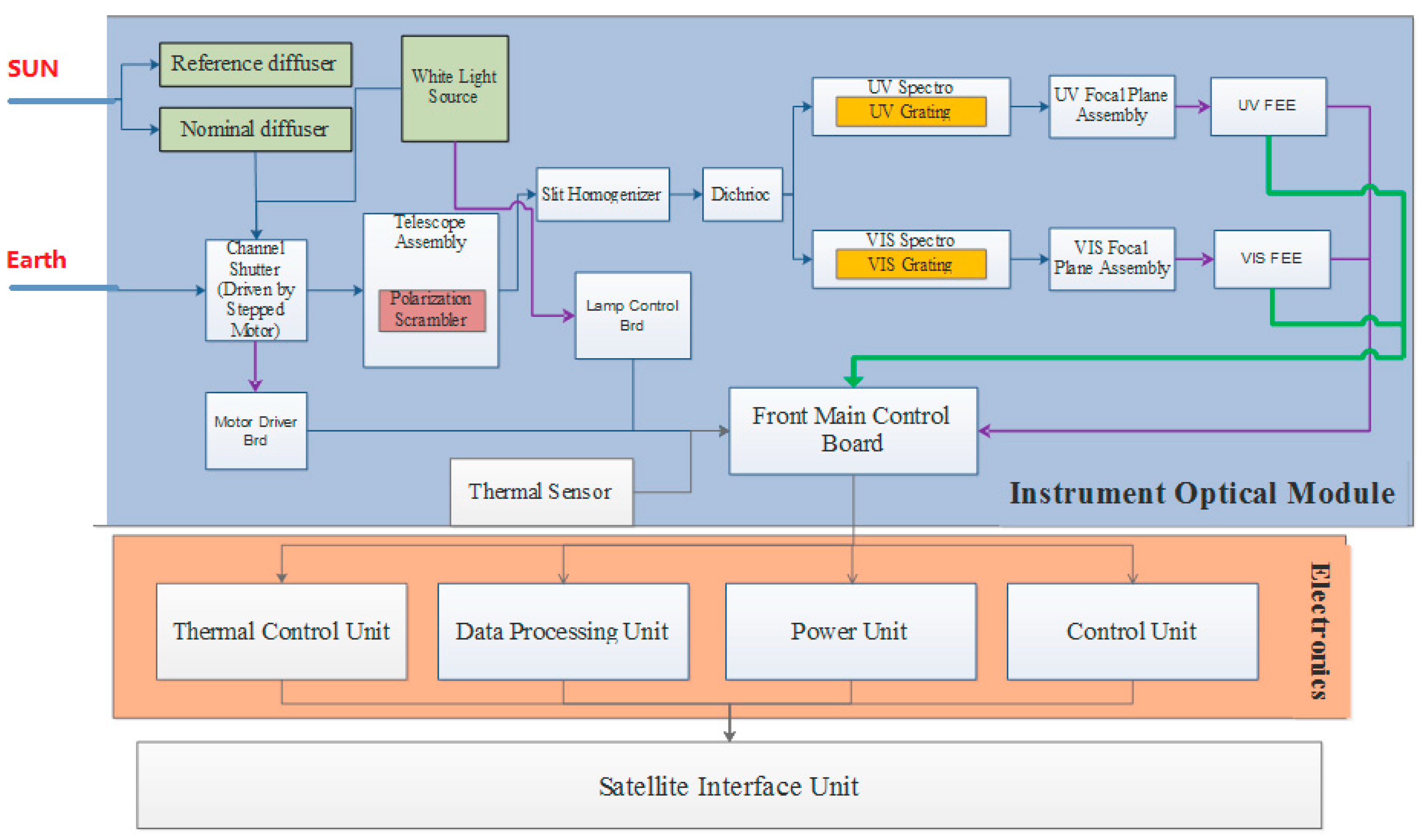
1.1. Overview

Environmental concerns have become paramount in the twenty-first century, with the depletion of atmospheric ozone, global warming, and acid rain ranking among the most pressing issues. Despite ozone’s minimal presence in the atmosphere, it is critical as a natural shield, protecting both humans and terrestrial organisms. Recent industrialization and increased human activities at higher altitudes have raised global concerns about ozone layer depletion due to human-induced factors. The discovery of the Antarctic ozone hole served as a stark warning, and since ozone is a significant greenhouse gas, monitoring its temporal and spatial fluctuations has become a focal point for environmental remote sensing. Satellite-based atmospheric ozone detection has gained wide acceptance due to its global coverage and all-weather capabilities. Accumulating continuous data on the worldwide distribution of atmospheric ozone serves as a crucial input for China’s environmental monitoring, climate forecasting, and global climate change research [1,2].

The evolution of the new generation of ozone detection instruments [3,4] highlights a notable trend: a shift from single atmospheric ozone measurements to the simultaneous measurement of various gas components, with ozone as the centerpiece. From a technical perspective, the widespread use of CCD devices and array devices, replacing photomultiplier tubes, has transformed the original discrete spectral observation into continuous spectral observation within the detection band range. This shift significantly enhances the precision of atmospheric ozone inversion. Additionally, to acquire information about tropospheric ozone, the instrument must be capable of ozone profile measurement.

The UVS dynamically monitors global total ozone levels by detecting atmospheric backscattered radiation in the solar ultraviolet and visible light spectra. Furthermore, it monitors crucial trace gasses associated with atmospheric ozone and the atmospheric environment, including SO2, NO2, BrO, HCHO, and OCLO, as well as aerosol optical thickness, cloud-top pressure, and ozone contours.

UVS incorporates three spectral channels: UV1 (250–300 nm), UV2 (300–320 nm), and UVIS (310–495 nm).

Table 1. Specifications of UVS.

Index	Characteristics
Scientific objectives	O3, SO2, NO2, BrO, O3 profile, Aerosol, Cloud, etc.
Channel	UV1	UV2	UVIS
Spectral range/nm	250–300 nm	300–320 nm	310–495 nm
Spectral resolution/nm	~1	0.5	~0.6
Field of view	112°
Spatial resolution	28 km × 21 km (at nadir)	7 km × 7 km (at nadir)	7 km × 7 km (at nadir)
SNR	>50	>200	>200@ UV >1000@ VIS
Wavelength calibration accuracy	0.05 nm	0.05 nm	0.05 nm
BRDF calibration accuracy	3%

summarizes key specifications of UVS.

Figure 1 shows a block diagram illustrating the operational principle of UVS. Atmospheric backscattered radiation enters the instrument through the primary mirror of the wide-angle telescope system, reflecting off the primary mirror, and is subsequently deflected by the depolarizer. The second mirror of the super wide-angle telescope system focuses the light onto the incident slit of the spectrometer. A dichroic mirror divides the light into two parts: UV1–UV2 channels and the UV-Vis channel. Both parts are directed through plane gratings and imaging objective lenses before being captured by CCD detectors. The detector’s one-dimensionality provides the required spectral distribution of ultraviolet/visible backscattered radiation from the Earth’s atmosphere, while the other dimension gives the spatial distribution in the cross-track direction. The remaining spatial distribution is determined by the satellite’s orbital motion.

To ensure stable operation over its 8-year lifespan, on-orbit calibration plays a pivotal role. To monitor variations in radiation response during orbit, an on-orbit solar calibration mode for UVS was designed. This mode employs the instrument’s in-flight diffusers to introduce solar radiation for detection. UVS incorporates two diffusers: a primary diffuse reflector for monthly solar and white light calibration, and a backup diffuser for monitoring changes in the primary diffuse reflector every six months while in orbit. Monitoring the degradation of UVS necessitates calibration of the angular characteristics and irradiance response of UVS². Additionally, wavelength shift monitoring is performed using solar Fraunhofer lines during solar calibration.

Passive radiator plates achieve cooling for the optical bench and detector module. The optical bench operates at a temperature of 293.15 ± 2 K, while the detector operates at an even lower temperature of −243 K.

1.2. Description of BRDF

To mitigate the inconsistency in the response of the remote sensors between elements, it is required to provide an in solar diffuser reflector-based on-planet calibration; the sun serves as a standard light source and illuminates the diffuser reflector, forming a uniform irradiance source. Additionally, relative corrections are introduced to the remote sensors to be calibrated.

The crucial component governing the bidirectional reflectance distribution function (BRDF) of the UVS instrument is the onboard diffuser [4,5]. This onboard diffuser facilitates the transformation of sun irradiance into radiance, measured subsequently by the instrument.

The BRDF (bidirectional reflectance distribution function) represents the micro-increment of surface irradiance reflected in a specific direction, expressed as the ratio between the incremental brightness of the reflected radiation and the incident irradiance.

Radiance is used to describe the intensity distribution of a radiation field. It represents the physical quantity of the strength of radiation at a point on a surface radiation source in a specific direction. The unit of radiance is μW/cm²/sr/nm. Irradiance refers to the radiant flux per unit area of the illuminated surface, with the unit being μW/cm². The BRDF of the diffuse reflection plate on the satellite can be defined as follows [6]:

$$E={\displaystyle \frac{L}{BRDF}}$$

(1)

where E denotes irradiance, and L denotes radiance, which can be expressed as follows:

$$L=A·S$$

(2)

where A denotes the radiance response of the load instrument, and S denotes the output count of the load detector.

The detection signals in the Earth mode are derived through two steps: first, using a solar simulator [7] and a standard diffuse reflector with a known BRDF, and secondly, by switching the instrumental operation mode to the solar mode. In the solar mode, the detection signals are obtained by using a simulated light source to directly illuminate the solar-port diffuse reflector. The bidirectional distribution function of the UVS diffuse reflection is derived by comparing these two signals, as shown in the following formula:

$$E={\displaystyle \frac{A·S_1}{BRD{F}_{diffuse}}}$$

(3)

where E denotes the input irradiance, A denotes the instrument radiance response, S₁ represents the detecting counts in the Earth mode, and $BRD{F}_{diffuse}$ represents the bidirectional reflectance distribution function of the standard diffuser.

In the solar mode, the input irradiance can be expressed as follows:

$$E={\displaystyle \frac{A·S_2}{BRD{F}_x}}$$

(4)

where S₂ represents the detecting counts in the solar operating mode, and $BRD{F}_x$ represents the bidirectional reflectance distribution function of the onboard diffuser. According to a comparison between Formulas (3) and (4),

$$BRD{F}_x={\displaystyle \frac{S_2}{S_1}}BRD{F}_{diffuse}$$

(5)

Throughout the year, as the sun moves along the ecliptic, the angle (α, β) between sunlight and the incidence window’s normal constantly changes; α represents the azimuthal angle of sunlight incidence, and β represents the pitch angle of sunlight incidence.

The radiometric calibration of the onboard system is crucial for ensuring the accuracy of target retrieval. The variability in the reflectance of the core component, i.e., the diffuse reflector, directly impacts the precision of radiometric calibration. To mitigate the impact of reflectance variability, a dual diffuse reflector system comprising a working board and a reference board (as shown in Figure 2a) is employed in this instrument. The calibration intervals for the dual diffuse reflector are set at once every 10 days and once per quarter. Each calibration session lasts approximately 2 min. The reference board is utilized to calibrate changes in performance exhibited by the working board. Considering potential environmental effects on the diffuse reflectors when radiometric calibration is not being conducted, both working and reference boards are stored in shaded areas where they are shielded from solar ultraviolet radiation when not in use.

The variations in β and α are determined by satellite orbit and launch window calculations, as depicted in Figure 2b. Accurately measuring the BRDF distribution characteristics of the diffusers requires assessing the bi-directional reflectance distribution function of the diffuser under various sunlight incidence angles (α, β) (here α and β are the angle between sunlight and the satellite’s flight direction, where the satellite’s flight direction is the direction normal to the ground of the L bracket) [8]. Therefore, adjusting the angle of the absorptive aerosol detector in the solar operation mode using a high-precision rotary table is necessary. The BRDF of the diffuser under different conditions is obtained using the aforementioned calculation method. The sun observation range of UVS is α ∈ [−4°, +4°], β ∈ [14.95°, 37.95°].

During solar calibration, the sun enters diffuser 1 at a specific angle and is then scattered directly onto the first mirror (M1) of the UVS optical path. The scattering angle covers the entire 112° field of view of the UVS, allowing for complete solar calibration data to be obtained one time.

2. Experiment

2.1. Equipment for Calibration

The primary equipment used for calibration included a dedicated oil-free vacuum system, ensuring the optical components of the instrument remained uncontaminated. The vacuum system maintained a level of 6 × 10⁻⁴ Pa, with a cleanliness rating of 1000. The UVS comprised a thermal control system to ensure that the temperature was consistent with the in-orbit conditions. A solar simulator was used to provide ultraviolet-visible collimated light. In addition, a five-dimensional mobile station was incorporated to provide various test positions and angles for the instrument, and a standard diffuser calibrated by NIST was adopted as a reference for the BRDF measurements. Additional auxiliary equipment was also used. All tests and calibrations had to be conducted within a clean room environment. Figure 3 and Figure 4 illustrate the schematic diagrams of the vacuum calibration testing system. The inner walls of the vacuum chamber were coated with a black, light-absorbing layer to minimize the impact of stray light. The super-black coating had a thickness of 50 um and exhibited a visible and infrared absorption rate of 0.98 ± 0.01. During calibration, we used liquid nitrogen to lower the temperature of the environment inside the tank, and the UVS was equipped with a temperature control system to ensure that the working environment during calibration matched that in orbit.

• Solar simulator

In laboratory radiometric calibration, we employed a 200 cm long solar simulator with a 20 cm diameter exit port. It featured a reflective off-axis optical design, with interior mirrors coated in UV high-reflection film. The simulator utilized a single 3000 W lamp as a light source. The key specifications are as follows:

Wavelength range: 250–1100 nm;

Light output caliber: 200 mm;

Non-uniformity: 1.5%;

Divergence angle: ±0.5°;

Power adjustment range: 0.4–0.8 solar constants (continuously adjustable);

Stability: 1%/h.

2.

Five-dimensional mobile station

The measured load was positioned on a five-dimensional mobile platform, enabling translation in three directions and rotation along two axes. Therefore, the platform facilitated field scanning, allowing calibration for each pixel on the image plane.

3.

Standard diffuser

The simulator emitted collimated light, and the standard irradiance of the light source was measured by a radiometer. Calibration of the radiance (sensitivity) of the load to be measured was achieved through the scattering of a standard diffuser plate. Key indicators of the standard diffuser plate are as follows:

Spectral range: 200–700 nm;

Reflectivity: >98% (250–500 nm);

Uniformity: greater than 95%;

Diffuser plate diameter: ≥150 mm × 150 mm;

Cosine characteristic error: ≤1%

As in Equation (5), the BRDF of UVS diffusers was calculated through transfer computations based on a NIST-calibrated standard diffuser.

2.2. Calibration Setup

The calibration process begins with the alignment of the solar simulator outlet surface and the diffuser’s reflective surface to be parallel. The spatial and spectral dimensions of the UVS detector are 512 × 1024. To improve the inversion accuracy, the BRDF is altered pixel by pixel during ground calibration. At the ground port, one irradiation can cover only 6–7 rows of pixels in the spatial dimension. To ensure that the spatial dimension of the FOV is entirely covered, the rotary table must be used to adjust the UVS multiple times. The specific adjustment steps are as follows.

• The centers of these two surfaces must be perpendicular to their respective planes, with a consistent distance of approximately L, in accordance with the standard irradiance calibration.
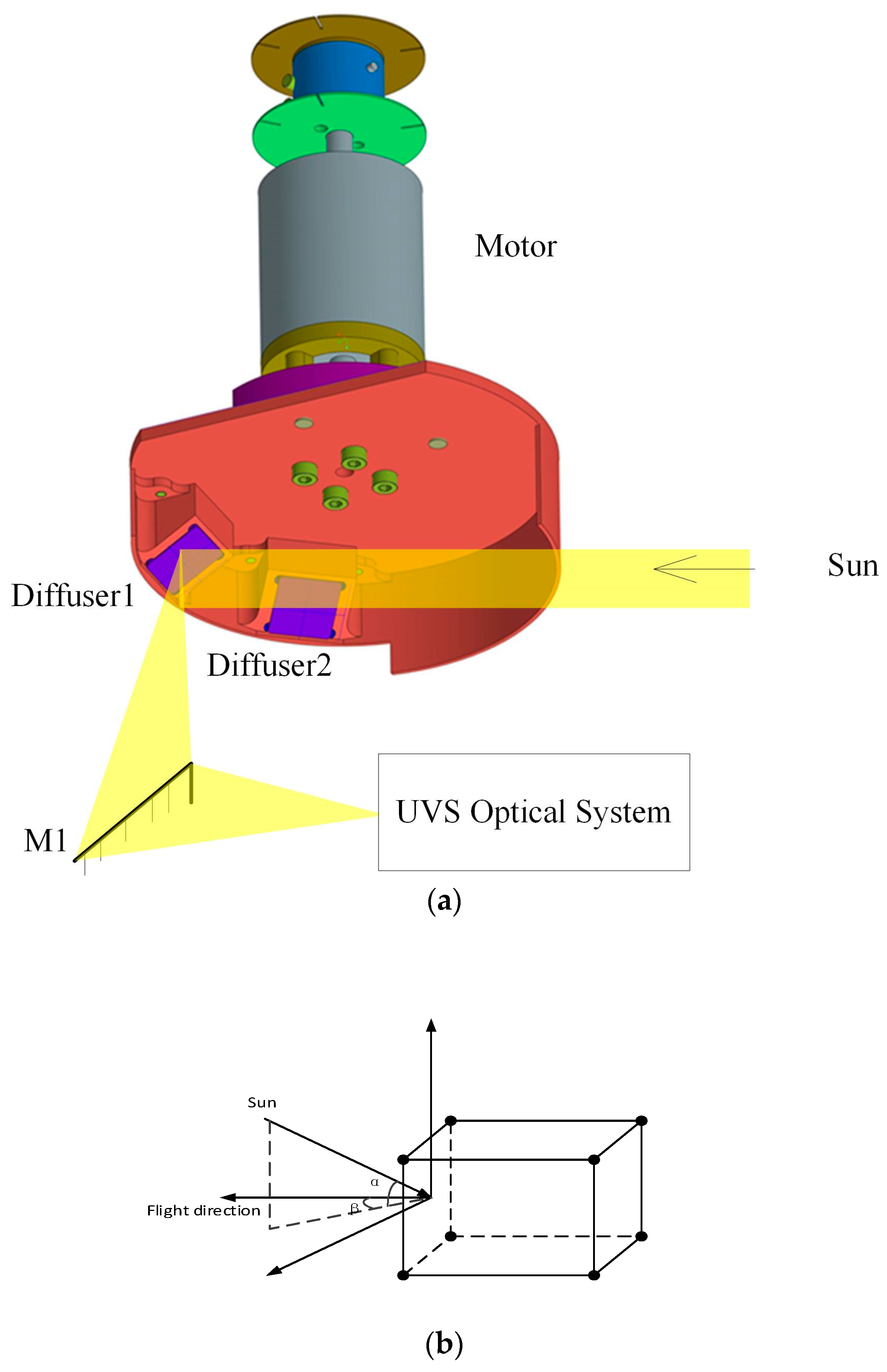
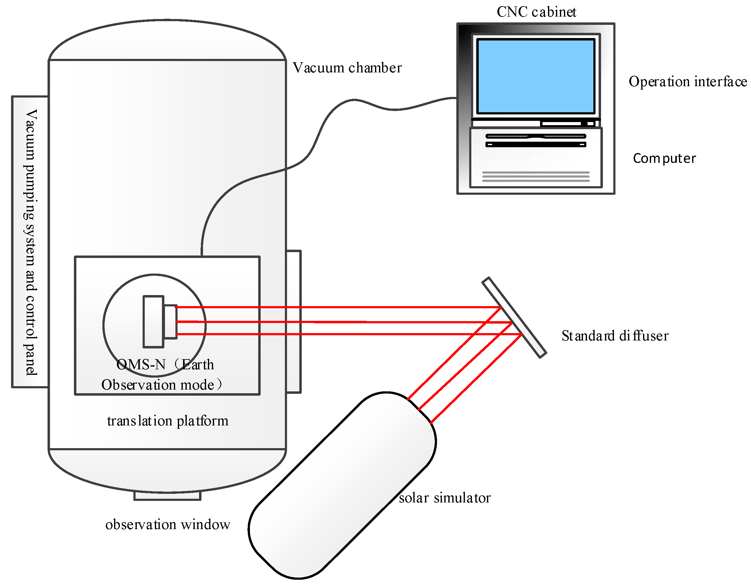
• This involves transitioning the UVS operational mode to “earth mode” to initiate observations of a designated point beneath the Earth’s surface. Adjustments are made to align the line connecting the center of the Earth port with the center of the diffuser to create a 30° angle with the normal of the diffuse reflector plate. Before commencing the calibration process, the light source is activated and allowed to stabilize for ten minutes.
• To capture comprehensive data, the rotation of the payload turntable begins, starting from the edge of the payload field of view (FOV) and progressing in 0.5° intervals until the instrument completes a full FOV scan. Ten observations are collected for each rotation position.
• Following this, the payload’s operational mode is transitioned to “solar mode”, and the onboard diffuse reflective plate is configured to “calibration 1” mode. The test apparatus is setup according to the provided diagram, ensuring that the front surface of the light source outlet aligns parallel to the sun port’s surface.
  Equal distances must be maintained between the optical stimulus and the onboard diffuser, both in the irradiance mode and the radiance mode, through careful adjustments.
• The angles are set to β = 26.45° and α = 0, and 50 data frames are acquired. α measurements start from −4°, adjusting in 1° increments up to +4°, with images captured at each α angle. Starting at 14.95°, β is measured in 1° increments up to 37.95°, and α is recorded at each β angle. Finally, the onboard diffuse reflector calibration board is transitioned to calibration 2 mode, and the test procedure is repeated to conclude the BRDF calibration for both onboard diffuse reflector boards.

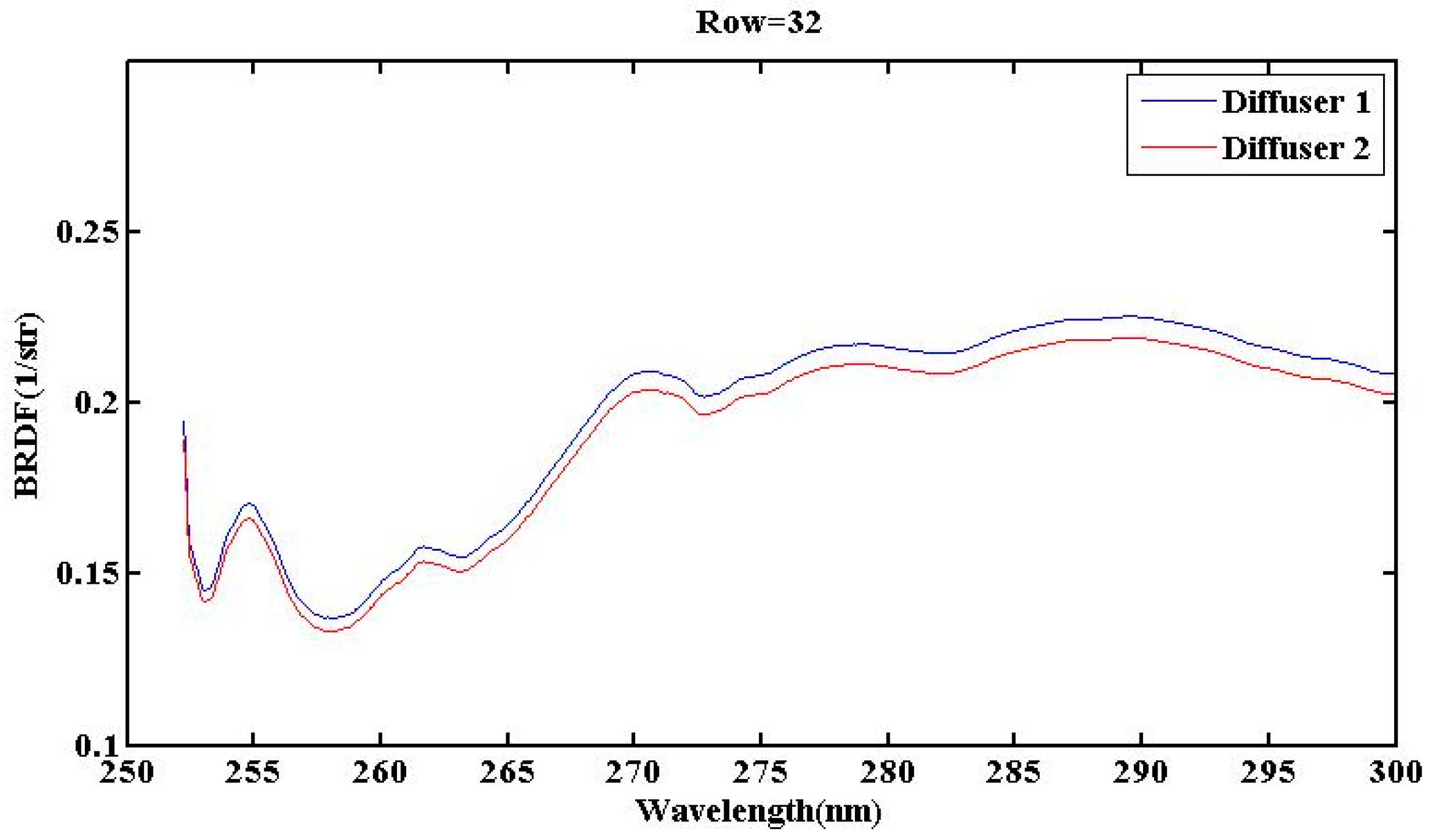
3. Results and Discussion

During the calibration process, we continuously monitored the temperature of the payload and changes in the dark background. The UVS CCD has a specific area designated for measuring the dark background, so during data processing, the background of the current image was subtracted accordingly.

The test data should be averaged based on the incident angle state, followed by subtraction of the dark background from the averaged data to obtain the ‘incident angle—DN’ dataset. The irradiance responsivity was determined using standard conversion values under various incident angle conditions. Per Formula 5, the BRDF of the NIST standard diffuser can be transformed into a set of “α-β-BRDF” data corresponding to various incident angles.

The BRDF is a function of wavelength (CCD column), viewing direction (CCD row), and the incident angles of the diffuser. For the results presented in this section, we focus on the normal azimuth (β = 26.45°) and elevation (α = 0.0°) angles. Under thermal-vacuum conditions, the BRDF of the UVS instrument was calibrated for a subset of viewing angles ranging from −56° to +56°. Figure 5, Figure 6 and Figure 7 depict the BRDF results for the UV1, UV2, and VIS channels at a viewing angle of 0° for the two onboard diffusers. Notably, these curves exhibit smooth variations across wavelengths. Figure 8 illustrates the BRDF for all pixels at the normal azimuth and elevation angles across the three channels.

The data series for the “α-β-BRDF” was fitted using a quadratic equation, as illustrated in Equation (6). In addition to satellite operations, the high correlation between the BRDF of UVS and azimuth and elevation angles must be considered. For each CCD pixel, a model [9] can be constructed as follows:

$$\begin{array}{ll}\mathrm{BRDF}(\mathrm{row},\mathrm{col})& =\mathrm{px}0\mathrm{y}0(\mathrm{row},\mathrm{col})+\mathrm{px}1\mathrm{y}0(\mathrm{row},\mathrm{col}).*\beta +\mathrm{px}0\mathrm{y}1(\mathrm{row},\mathrm{col})·\alpha \\ & +\mathrm{px}2\mathrm{y}0(\mathrm{row},\mathrm{col})·{\beta }^2+\mathrm{px}1\mathrm{y}1(\mathrm{row},\mathrm{col})·\beta ·\alpha +\mathrm{px}0\mathrm{y}2(\mathrm{row},\mathrm{col})·{\alpha }^2\end{array}$$

(6)

where $\mathrm{px}0\mathrm{y}0$, $\mathrm{px}0\mathrm{y}1$, $\mathrm{px}2\mathrm{y}0$, $\mathrm{px}1\mathrm{y}1$, and $\mathrm{px}0\mathrm{y}2$ are coefficients.

The fitted surface depicts the correlation between the UVS diffuse BRDF and various α and β angles. Figure 9 illustrates the BRDF of diffuser 1 at different azimuth and elevation angles across the three channels. The BRDF, in conjunction with azimuth and elevation angles, conforms well to a quadratic equation. Figure 10 and Figure 11 displays the six coefficients of the fitted curves for all pixels of the two diffusers.

Given that the same light source is considered in the Earth and solar mode calibrations at equal distances, the irradiance of the light source can be neglected according to the forward Formula (5). Various sources contribute to the uncertainty in the BRDF calibration process for the satellite-mounted diffuse reflector panels, including source non-uniformity, standard diffuser plate uncertainty, UVS non-stationarity, source non-stationarity, and solar simulator distance.

The absolute accuracy of the UVS encompasses factors such as the standard diffuser plate uncertainty at the National Institute of Metrology (NIM), UVS non-stationarity, source non-uniformity (including source angle non-uniformity and source plane non-uniformity), source non-stationarity, and solar simulator distance error. The error can be calculated using Formula (7).

Table 2. Diffuse reflector calibration uncertainty.

	UV1	UV2	VIS
Source non-uniformity	1.5%	1. 5%	1.5%
Standard diffuser plate uncertainty	1%	1%	1%
UVS non-stationarity	0.42%	0.42%	0.47%
Source non-stationarity	1%	1%	1%
Solar simulator distance error	0.5%	0.5%	0.5%
Total	2.162%	2.162%	2.173%

summarizes these results.

$$\delta =\sqrt{{x_1}^2+{x_2}^2+{x_3}^2+{x_4}^2\cdots +{x_n}^2}\times 100\%$$

(7)

where $\delta$ denotes the total uncertainty, and x_n denotes the uncertainty of each sub-component. The total uncertainty in the calibration is summarized in Table 2.

The final accuracy for the UVS absolute BRDF calibration parameters, as determined on the ground using the methods described above, is less than 3%. This uncertainty arises from variations between measurements obtained with different external light sources.

4. Conclusions

In this study, we calibrated the bidirectional reflectance distribution function (BRDF) by simulating incidence angles in orbit and testing the BRDF for various angles.

In Section 3, we utilized a transfer formula to calculate the relationship between the UVS BRDF under different incidence angles. The results indicate that, at specific incidence angles, the BRDF exhibits wavelength-dependent and spatial distribution characteristics, leading to varying BRDF characteristics corresponding to each pixel on the CCD image plane. From the results, it is evident that the diffuser’s dependence on wavelength is more pronounced in the 250–300 nm compared to the 300–500 nm. The BRDF characteristics of the diffusers of the UVS were evaluated. Based on radiometric calibrations involving multiple azimuth and elevation angles, a BRDF model was established for each pixel, revealing coefficients for the two diffusers in UVS. From the perspective of spatial distribution at a specific angle, the changes in BRDF are not entirely uniform across a wide field of view, and this phenomenon may be attributed to the intrinsic characteristics of the diffuse reflection board material. Given that all pixels on the UVS have been calibrated, these wavelength-dependent and spatially dependent characteristics can be adjusted through calibration coefficients.

We conducted a comprehensive analysis and precise calculation of the uncertainties inherent in the calibration process. The accuracy levels of UVS in the UV1, UV2, and VIS channels were 2.162%, 2.162%, and 2.173%, respectively. The coefficients obtained from the fitting serve as the baseline coefficients for the in-orbit testing of the UVS. The UVS BRDF calibration was conducted under simulated in-orbit conditions, including the environment and operational modes, so the obtained calibration coefficients can be directly used for the initial in-orbit phase. Subsequent validation and analysis will be carried out using the corresponding solar data. Future studies are warranted to improve the BRDF model based on in-orbit comparison results.

References

- Butler, J.J.; Park, H.; Barnes, P.Y.; Early, E.A.; van Eijk-Olij, C.; Zoutman, A.R.; van Buller-Leeuwen, S.; Schaarsberg, J.G. Comparison of ultraviolet bidirectional reflectance distribution function (BRDF) measurements of diffusers used in the calibration of the Total Ozone Mapping Spectrometer (TOMS). In Proceedings of the International Symposium on Remote Sensing, Crete, Greece, 23–27 September 2002. [Google Scholar]
- Smorenburg, K.; van Valkenburg, A.L.G.; Werij, H.G.C. Absolute radiometric calibration facility. In Proceedings of the Satellite Remote Sensing II, Paris, France, 25–28 September 1995. [Google Scholar]
- Wohltmann, I.; Barry, B.; Klein, U.; Langer, J.; Lindner, K.; Kunzi, K.F.; von der Gathen, P. Comparison of ozone measuring instruments in Ny-lesund, Spitsbergen. In Proceedings of the Fifth European Symposium, Saint Jean de Luz, France, 27 September–1 October 1999. [Google Scholar]
- Lumpe, J.D.; Alfred, J.M.; Shettle, E.P.; Bevilacqua, R.M. Ten years of Southern Hemisphere polar mesospheric cloud observations from the Polar Ozone and Aerosol Measurement instruments. J. Geophys. Res. Atmos. 2008, 113, D04205. [Google Scholar] [CrossRef]
- de Vries, J.; van den Oord, G.H.J.; Hilsenrath, E.; te Plate, M.B.J.; Levelt, P.F.; Dirksen, R. Ozone monitoring instrument (OMI). In Proceedings of the SPIE Conference Imaging Spectrometry VII, San Diego, CA, USA, 29 July–3 August 2001. [Google Scholar]
- Hilker, T.; Coops, N.C.; Hall, F.G.; Black, T.A.; Wulder, M.A.; Nesic, Z.; Krishnan, P. Separating physiologically and directionally induced changes in PRI using BRDF models. Remote Sens. Environ. 2008, 112, 2777–2788. [Google Scholar] [CrossRef]
- Kleipool, Q.; Ludewig, A.; Babić, L.; Bartstra, R.; Braak, R.; Dierssen, W.; Dewitte, P.J.; Kenter, P.; Landzaat, R.; Leloux, J.; et al. Pre-launch calibration results of the TROPOMI payload on-board the Sentinel 5 Precursor satellite. Atmos. Meas. Tech. 2018, 11, 6439–6479. [Google Scholar] [CrossRef]
- Lawrence, J.; Rusinkiewicz, S.; Ramamoorthi, R. Efficient BRDF importance sampling using a factored representation. In Proceedings of the Special Interest Group on Computer Graphics and Interactive Techniques, Los Angeles, CA, USA, 8–12 August 2004. [Google Scholar]
- Schlick, C. An inexpensive BRDF model for physically-based rendering. Comput. Graph. Forum 1994, 13, 233–246. [Google Scholar] [CrossRef]