Abstract
This study numerically investigated the effects of various contact strategies on the thermal hydraulic behavior within a structured bed of 100 explicitly modeled pebbles. Four contact strategies and two thermal hydraulic conditions were considered. The strategies to avoid contact singularities include decreasing the pebble diameter, increasing the pebble diameter, bridging the pebble surfaces near the contact region, and capping the pebble surfaces near the contact region. One strategy, Strategy 3a, which involves bridging with a cylinder equal to 10% of the pebble diameter, was selected as the baseline strategy because it addressed the contact singularity while minimizing the geometric changes that affect the bed porosity. The two thermal hydraulic conditions were full-power operation (Case 1) and pressurized loss of forced cooling or PLOFC (Case 2). Simulations of the conjugate heat transfer within the structured bed were performed using the Reynolds-averaged Navier–Stokes approach with the realizable k- turbulence model and two-layer all wall treatment. The thermal-fluid quantities of interest were compared between the contact strategies for each case. In Case 1, the hydraulic behavior was sensitive to the contact strategy, with large differences in the pressure drop (30%) and volume-average velocity (4%). The thermal behavior was not sensitive, with less than a 0.5% difference across the strategies. To better understand the separate effects of each heat transfer mode, Case 2 was divided into the following subcases: conduction (Case 2a); conduction/radiation (Case 2b); and conduction/radiation/convection (Case 2c). Case 2a represents an early phase of the PLOFC transient. Case 2b represents an intermediate phase of the PLOFC transient, with the pebble temperatures sufficiently high for the radiative heat transfer to be non-negligible. Case 2c represents a late phase of the PLOFC transient after the establishment of the natural circulation of the heat transfer fluid. For Case 2, large differences in the contact strategy were observed only in Case 2a with only conduction. The difference in the maximum pebble temperature was 23% in Case 2a, 2% in Case 2b, and 0.3% in Case 2c.
1. Introduction
The primary objective of this study was to identify the optimal strategy to address the point-contact singularity commonly encountered when explicitly modeling pebble-bed reactor cores for computational fluid dynamics (CFD) simulations. Pebbles modeled as perfect spheres within structured or unstructured beds are in point-contact configurations with the adjacent pebbles (particle–particle) as well as internal reactor vessel and neutron reflector surfaces (particle–wall). This effort investigated structured beds.
While unstructured bed flow fields are different, the contact strategy options are the same regardless of if the beds are structured or unstructured. The most desirable contact strategies are those that prioritize minimizing the porosity error as much as possible while providing a thermal connection to enable specifying an effective point-contact thermal resistance. Therefore, the recommended contact strategies and sizing selection are expected to hold for unstructured beds. Also, a study investigating externally heated unstructured beds reached similar conclusions as this effort with internally heated pebbles regarding the opportunity cost of each strategy and the sizing recommendations [1].
However, the overall conclusions are expected to hold for unstructured beds. Such point singularities must be avoided to discretize the computational domain into finite-volume elements. The commonly used techniques to avoid these point contacts can be placed into two groups, which either decrease or increase the pebble volume. The methods that decrease the volume include decreasing the pebble diameter or chamfering the pebble near the point contact. Decreasing the pebble diameter is the most straightforward approach for model building, the least difficult to mesh, and often the preferred starting point. The first 3D explicitly modeled pebble bed with simultaneous heat transfer and fluid flow was investigated in 2004 via a pebble diametral reduction [2]. At that time, and today, the experimental techniques lack the ability to provide detailed local heat transfer measurements for contact strategy validation. The quasi-direct numerical simulation (DNS) results of a single face-centered cubic (FCC) unit cell were generated for model development and validation [3]. These quasi-DNS results used the diametral reduction strategy to avoid the point-contact singularity. The authors mentioned that their objective was to keep the inter-pebble gap reasonably small while adhering to the DNS mesh constraints. A 4.2% diametral reduction was chosen, a significantly greater decrease than the values studied in this paper (0.1–1%). The diametral reduction strategy is still used today in modern large-eddy simulation (LES) approaches with thousands of explicitly modeled pebbles [4] and DNS simulations with up to 150 pebbles [5]. Such a global geometric change was recognized to significantly alter the bed porosity and pressure drop [1]. Therefore, local geometric modifications are also of interest. The capping method involves chamfering the contacting pebbles and filling the chamfered volume with fluid [6].
There are also global and local increase volume methods that include increasing the pebble diameter or chamfering the contacting pebbles near the point contact and filling the nearby volume with a bridge of solid pebble material. Eleven explicitly modeled pebble beds were studied using global diametral increases [7,8]. However, a range of values did not consider estimating the sensitivity of the diametral increase and making suggestions about the desired amount of overlap. Two disadvantages of the diametral increase strategy include (1) having the potential to introduce new contacts with nearby adjacent pebbles, and (2) the fluid domain meshing is still complex in the small interstices near the original point-contact singularity [1].
Each method has a unique impact on the thermal hydraulic behavior of the bed. Therefore, the optimal contact strategy may not be the same for all the reactor conditions where the dominant mode of heat transfer changes from forced convection (steady-state full-power operation) to either conduction- or radiation-dominant. In this study, point-contact strategies were investigated for full-power operation at a typical pebble power density and for a pressurized loss of forced cooling (PLOFC) with a reactor trip event. Each contact strategy is illustrated in Figure 1.

Figure 1.
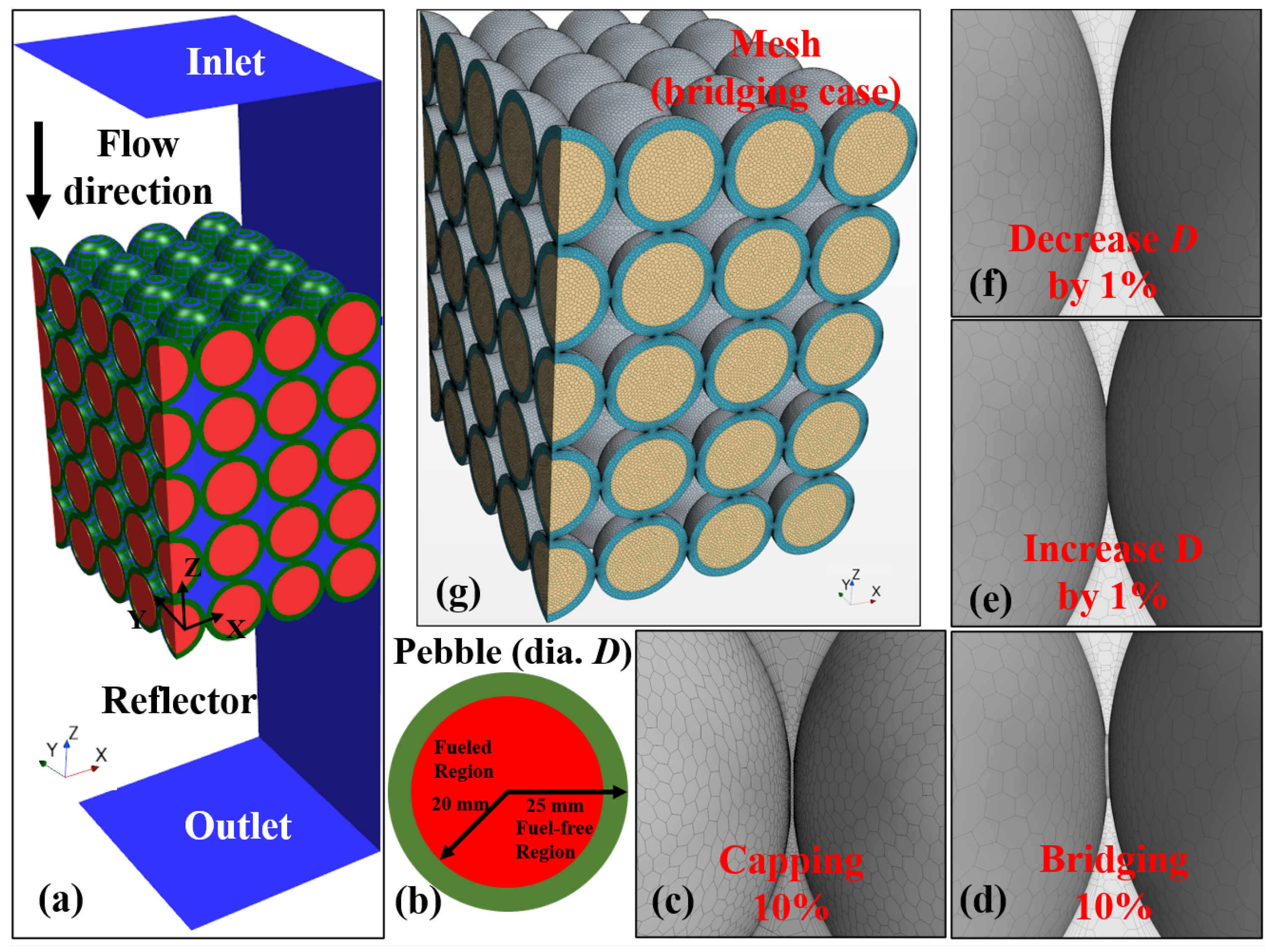
(a) Computational domain consisting of a structured bed of 100 explicitly modeled pebbles with (b) pebble dimensions. Strategies for point contacts with adjacent pebbles consist of (c) capping, (d) bridging, (e) increasing the diameter, and (f) decreasing the diameter. (g) A mesh of the bridging strategy.
- Strategy 1 (a-b-c): Decreasing the pebble diameter by , , and . This is a simple model-building approach of slightly decreasing the pebble diameter. Decreasing the pebble by was the most computationally expensive approach due to the very small gaps between the pebbles.
- Strategy 2 (a-b-c): Increasing the pebble diameter by , , and .
- Strategy 3 (a-b-c): Bridging—that is, chamfering contact pebbles with a given diameter (, , and in this study) and filling the volume with pebble material. This approach was considered the most similar to the true bed configuration when comparing its porosity to the true value, and thus it was selected as the baseline for comparison.
- Strategy 4 (a-b-c): Capping—that is, chamfering contact pebbles with a given diameter (, , and in this study).
Two reactor operating conditions were investigated for each contact strategy: (Case 1) full power and (Case 2) PLOFC. The Case 1 power density of is prototypical of full-power operation for tristructural isotropic (TRISO) fuel forms using high-assay low-enriched uranium and helium gas as the heat transport fluid [9]. The associated full-power values were specified as boundary conditions, including a 3 m/s−1 fluid inlet velocity, a 250 °C inlet temperature, and an outlet pressure of 6 . Case 2 roughly corresponds to the PLOFC with a reactor trip event, and this case was motivated by an objective to better understand the contact strategy under the separate effects of each heat transfer mode of conduction, convection, and radiation. For this case, the pebbles were assumed to have a temporally constant power density equal to of the full-power density, which corresponds to approximately 20 s after the reactor trip [10].
Instead of temporally resolving the PLOFC transient, the event was divided into three unique and steady subcases that correspond to the distinct scenarios of the event. Case 2a represented a phase of the PLOFC transient when the heat transport fluid reaches a near-zero velocity during the expected flow reversal phenomena after circulator pump coastdown and control rod scram [11]. Case 2a only considered conduction as a means of energy transport to study how different the temperature and heat flux fields would be between contact strategies that result in pebble overlaps (Strategies 2 and 3) or pebble gaps (Strategies 1 and 4). In Case 2a, the pebble surface temperatures reached sufficiently high temperatures that would make thermal radiation a non-negligible mode of energy transport. Therefore, Case 2b included radiative heat transfer. Case 2c represented a late phase of the PLOFC transient after the establishment of the buoyancy-driven natural circulation of the heat transfer fluid. This case captured the contact strategy behavior when conduction, convection, and radiation occur simultaneously.
In this work, the pore-scale hydraulic diameter () and pore Reynolds number () are defined as
where is the calculated porosity for each contact strategy, is the pebble diameter, and and are the density and dynamic viscosity of the heat transfer fluid (helium gas), respectively. is the average interstitial velocity between the pores related to the superficial velocity, U, through . The superficial velocity or the Darcian flow is defined as , where Q is the volumetric flow rate, and A is the cross-sectional area of an empty bed.
The heat transfer coefficient and the Nusselt number are defined as
where is the pebble surface heat flux, and and are the volume-averaged pebble surface and fluid temperature. The fluid thermal conductivity is denoted as .
For each contact strategy, the calculated porosity, , was compared to an analytically computed true porosity using perfectly spherical pebbles with point singularity contact. Table 1 summarizes the total pebble volume, calculated porosity, pore-scale hydraulic diameter, and the porosity error for each contact strategy relative to the true porosity. Some of the tested contact strategies yielded a significant porosity error relative to the true porosity. Decreasing or increasing the pebble diameter by yielded a porosity error of . The bridging method with the smallest bridge diameter, equal to of the pebble diameter, showed the smallest porosity error of . This strategy (Strategy 3a (bridge 10%)) was used as the baseline numerical result against which all the other strategies were compared. Strategy 2a, increasing the pebble diameter by 0.1%, yielded a small porosity error, but the simulations were not numerically stable unless a significantly finer mesh than required for the other strategies was used. Therefore, the results of this strategy were not discussed and denoted as not available where applicable.

Table 1.
Calculated porosity, pore-scale hydraulic diameter , and porosity error relative to the true porosity for four different pebble contact strategies of various sizes.
STAR-CCM+ v16.02.009, a commercial finite-volume CFD software package developed by Siemens (Munich, Germany), was selected for this study. A steady Reynolds-averaged Navier–Stokes (RANS)-based approach to turbulence modeling was chosen for this effort given the size of the domain of interest and the available computational resources. This approach was chosen to maximize the accuracy of the numerical solution for conjugate heat transfer while balancing the relative computational costs to the porous media, large-eddy simulation, and direct numerical simulation methods.
2. Materials and Methods
2.1. Numerical Domain and Material Properties
Figure 1 presents the computational domain used in this study. A total of 100 pebbles were explicitly modeled using a structured array. Each pebble consisted of a fuel sphere surrounded by a fuel-free spherical shell. The fuel region represented a homogenization of TRISO particles within a graphite matrix. This region was defined as the power-producing volume with spatially constant volumetric heat sources (Figure 1b). Before making geometric modifications, the fuel region diameter, , was 0.04 m, and the fuel-free region outer diameter, , was 0.05 m. The heat transfer fluid inlet was located at the top of the domain, and the fluid outlet was located at the bottom. Three vertical planar slices were created to the domain to establish surfaces for symmetric boundary conditions. The resulting bed contained 45 whole pebbles and 55 sliced pebbles. The fourth vertical surface of the domain represented a radial reflector wall that was in contact with the pebbles. This surface was specified with a no-slip hydraulic boundary, a convective heat transfer coefficient of 10 W/(mK), and a 250 °C ambient temperature to approximate the thermal pathway through a radial reflector and reactor vessel to a prototypical gas-cooled reactor cavity.
All boundary and interfacial conditions are specified in Table 2 for each region. The inlet turbulence parameters of turbulent kinetic energy, turbulent dissipation rate, turbulent viscosity, and turbulent thermal diffusivity were derived from the inlet specifications of 0.01 and 10 for turbulence intensity and turbulent viscosity ratio, respectively.
Table 2.
Boundary and interfacial conditions.
The material properties, except the fluid density, were specified at 6 MPa and 250 °C. These are independent of temperature and position within the computational domain and are presented in Table 3. The fluid density was determined using a compressible flow solver and the ideal gas approximation. Also, the thermal contact resistance between pebbles was ignored, and the pebble chamfer bridges were treated as if they were made of the same material as the pebble fuel-free region. It is apparent and expected that pebble temperatures are sensitive to how the near-wall region of the fluid domain is treated. Conjugate heat transfer problems require both the velocity and thermal boundary layers to be appropriately resolved. The ratio of these boundary layer thicknesses can be estimated by the molecular Prandtl number, represented as
where is the fluid-specific heat capacity, is the fluid-dynamic viscosity, and is the fluid thermal conductivity and yields a of 0.664. This implies that the velocity boundary layer thickness is slightly less than the thermal boundary layer thickness. From a domain discretization standpoint, the conclusion can be made that the grid resolution requirements to accurately capture the near-wall velocity and temperature gradients are relatively similar.
Table 3.
Specified temperature- and fluence-independent material properties.
2.2. Numerical Solvers
The heat-transfer and fluid-flow physics were coupled in a segregated manner of energy and flow transport. A detailed sensitivity study of turbulence models has been investigated but is not presented here in detail because discussions regarding RANS [13], unsteady Reynolds-averaged Navier–Stokes (URANS) [14], hybrid RANS/LES [15], and DNS [16] turbulence modeling comparisons already exist in the literature for body-centered cubic, face-centered cubic, structured, and unstructured. Most of the non-linear numerical methods generally predict similar mean velocity and temperature fields but differ significantly on the prediction of the root mean square (RMS) velocity and temperature fields with the bed. It has been suggested that the reason for poor RMS agreement is related to a significant amount of transitional flow affected by the pebble curvature.
However, validation data are lacking that are available to perform a thorough evaluation of turbulence modeling for the pebble-bed reactor application. Singular experimental configurations of heated beds that enable simultaneous measurement of temperature and time-resolved velocity fields are not easily accomplished. Prior isothermal efforts focused on particle image velocimetry (PIV) for time-resolved velocimetry [17,18] but lack temperature gradients.
In this study, RANS standard k-, realizable k-, and k- SST models were investigated. Relative differences in the predicted mean velocity fields between these three models could be decreased by
- Enabling the standard k- cubic constitutive relationship to improve anisotopic turbulence prediction of secondary flows and streamline curvature [19].
- Enabing the k- SST cubic constitutive relationship [20,21], which adds non-linear functional representations of the strain and vorticity tensors.
Across these closure models, the volume-averaged mean velocity field and bed pressure drop spanned ±4% and the volume-averaged mean pebble fuel temperature spanned ±2%. The steady RANS realizable k- turbulence model [22] with a second-order convection scheme, secondary gradients, and Wolfstein shear-driven two-layer all wall treatment [23] were selected. This decision was based on its wide applicability and the performance observed by Shams et al. [14] with acceptable agreement of mean fields with higher-order methods.
It is important to note that, regardless of the span of absolute values of velocity, pressure, and temperature fields, the conclusions regarding the geometric approach and selection of point-contact strategies remain unaffected.
The turbulent fluid motion and heat transfer are governed by mass continuity, solid energy conservation, fluid energy conservation, Navier–Stokes, and Poisson equations, provided as
where is the fluid velocity vector, is the solid density, is the solid specific heat capacity, T is the solid temperature, is the solid heat flux vector, is the solid convective velocity, is the solid volumetric heat source, is the fluid density, E is the fluid total energy, H is the fluid total enthalpy, is the fluid heat flux vector, isthe viscous stress tensor, is the fluid body force vector, is the fluid enthalpy of component i, is the diffusive flux of component i, is the fluid volumetric heat source, P is the fluid internal pressure, t is time, is the spatial coordinate vectors of component i, and is the fluid kinematic viscosity.
The steady RANS-based approach to turbulence modeling was chosen for this study due to its relatively low computational cost to porous media when compared to that of LES and DNS. The temporal averaging methodology, or Reynolds decomposition process [24], suggested by Osborne Reynolds was to separate fluid variables into their time-averaged mean and fluctuating components. Applying this process to Equations (6)–(10) yields
After the Reynolds decomposition of the Navier–Stokes equations, a closure problem is required to model the Reynolds stress tensor, . In this study, the applied closure method is the realizable model containing a new transport equation for the turbulent dissipation rate [22]. The transport equations for the kinetic energy k and the turbulent dissipation rate are
where is the mean fluid velocity vector and is the fluid turbulent kinematic viscosity. , , , and are model coefficients, and are production terms, is a damping function, is the large-eddy time scale, is the ambient source term time scale, and are the user-specified source terms, and is the ambient turbulence value in the source terms that counteracts turbulence decay.
For conjugate heat transfer of conduction and convection, the numerical method within STAR-CCM+ for adjacent fluid/solid cells create a fluid/solid contact interface and conserves the total heat flux. The heat flux is linearized with the following form:
where A, B, C, and D are net wall heat flux coefficients, is the bulk fluid temperature, and is the interfacial temperature. The heat transfer coefficient is defined locally based on the local flow conditions (fluid density, specific heat capacity, wall shear stress, and local Reynolds number), local fluid temperature, and local solid temperature. And this results in a local heat transfer coefficient for each cell face along the interface [23].
In Case 2, PLOFC, thermal radiative heat transfer was also modeled using the surface radiation exchange model (S2S) [23]. The heat transport fluid was assumed to be non-participating with no internal absorption, emission, or scatter (100% transparent to thermal radiation). The pebble wetted surfaces were assigned as the participating faces for thermal radiation, and these were used to calculate the appropriate view factors. No radiative heat transfer was modeled within the solid pebbles (100% opaque).
The radiation exchange between surfaces can be accounted for by tracking the amount of energy emitted from and absorbed from pairs of surface mesh faces as
where is the power emitted from face 1 and absorbed by face 2, is radiation intensity flux per unit area and per unit steradian, is the angle between faces, and L is the distance between faces.
Conservation of radiative energy is balanced only when using a closed set of surfaces. The total energy transfer can be calculated by summing over all faces that represent the closed set. For face i, this becomes
where and are the indexed face surface areas, is the indexed radiation flux, is the total number of faces, is the view factor from face j to i, is the diffuse component of radiation leaving face j, is the view factor from the environment to face i, is the transmissivity, and is the specular component of radiation. Other radiative assumptions included
- Each pebble surface mesh face was used in the view factor calculation;
- Gray radiation with no wavelength dependence;
- Diffuse radiation with no angular emission dependence;
- The effective radiation temperature of the environment was specified as 250 °C;
- A pebble surface emissivity of 0.8; and
- Satisfaction of Kirchhoff’s Law, such that emissivity + reflectivity + transmissivity = 1. This forces the surface reflectivity to 0.2 because the transmissivity is 0.
2.3. Mesh Sensitivity
Tetrahedral, hexahedral, and polyhedral mesh generation approaches were tested for each contact strategy. The bridging and diametral increase strategies resulted in a singular, complex body of all the fuel-free spherical shell regions. The parallel load distribution step required more computational time to decompose this body across the compute nodes. The capping and diametral decrease strategies resulted in many simple bodies. These geometries were significantly faster for interfacial definition (imprinting) and parallel discretization.
Fully conformal meshes were generated using polyhedral and prism layer meshing operations. The Surface Remesher performed surface vertex re-tessellation of the 3D CAD to optimize surface faces based on the target edge length and proximity refinements. In the Polyhedral Mesher process, a tetrahedral mesh is first generated for the input surface. Second, the polyhedral mesh is generated from the underlying tetrahedral mesh. The Prism Layer Mesher generated a subsurface to extrude a set of prismatic cells from the solid–fluid interfaces into the core mesh of the fluid region.
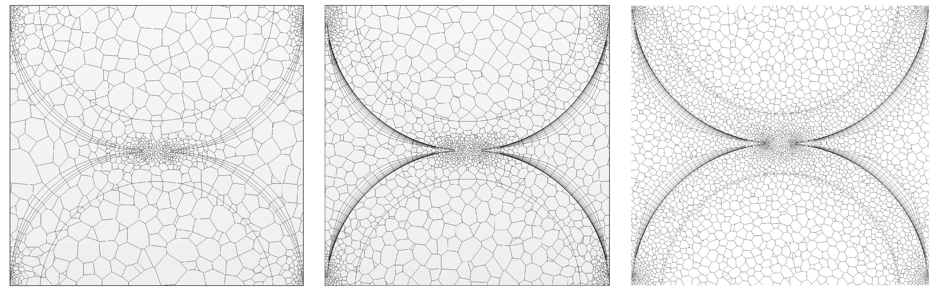
The sensitivity of the discretization on fluid flow and heat transfer behavior was quantified by performing mesh sensitivity studies for Cases 1–2. The Case 1 study is discussed in detail for each contact strategy. The diametral increase and bridging strategies had similar grid requirements. The diametral decrease and capping strategies required additional grid refinement to improve the prediction of the local velocity gradient in the small fluid pathways near the contact point. This refinement was also needed to achieve mesh independence for the pressure drop across the bed. For brevity, only the results from the bridging strategy are presented here. Coarse, medium, and fine meshes were generated using base cell sizes of 10 mm, 2 mm, and mm, respectively. The resulting numbers of cells for each mesh were , , and . Figure 2 presents cross-sections of the bed for each mesh resolution.
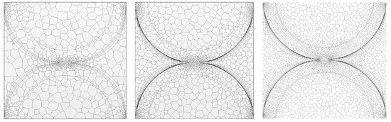
Figure 2.
Cross-sectional views of (left) coarse, (middle) medium, and (right) fine meshes used in the mesh sensitivity study for Strategy 3 (bridging).
To evaluate the numerical discretization error, estimate the rate of grid convergence, and determine an acceptable mesh density for this problem, the widely accepted Richardson extrapolation technique [25] was used. Quantities of interest (QOIs) were selected to quantify the grid convergence:
- Volume-averaged pebble fuel temperature, ;
- Maximum pebble fuel temperature, ;
- Volume-averaged fluid temperature, ;
- Volume-averaged fluid velocity magnitude, ;
- Maximum fluid velocity magnitude, ;
- Surface-averaged fluid temperature on plane Z2 (z = 0.1 m), ;
- Surface-averaged fluid velocity magnitude on plane Z2 (z = 0.1 m), ;
- The pressure drop across the entire bed, .
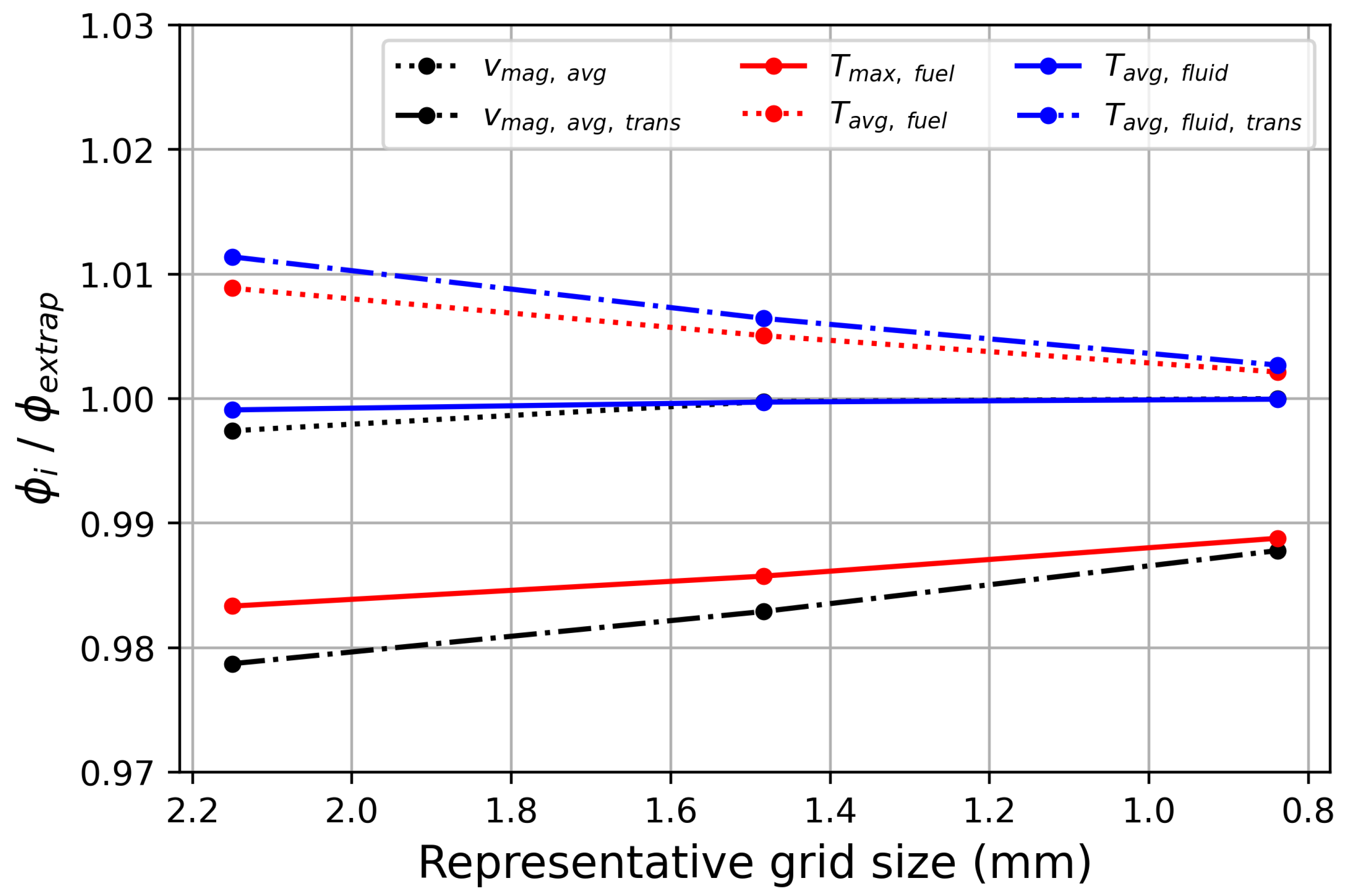
The convergence of each QOI, , is shown in Figure 3 as a function of a 3D unstructured grid representative cell size, h, and normalized by the extrapolated QOI with an infinite grid density, . For the coarse, medium, and fine meshes, was defined as 2.15, 1.50, and 0.84 mm, respectively, using the definition of

Figure 3.
Convergence of quantities of interest (QOIs) as the mesh was refined for Strategy 3 (bridging).
Macroscopic QOIs, such as the volume-averaged metrics, had similar behavior and rates of convergence across the various contact strategies. For the coarse mesh, all relevant QOIs were within 3% of an extrapolated solution with an infinite grid density, except for the velocity magnitude selected at an arbitrary point in the bed. This discretization error was reduced to nearly 1% for all QOIs for the fine mesh.
It is important to note that , a point-wise QOI, was selected at an arbitrary coordinate in the bed and was not held spatially constant. Also, the polyhedral mesh refinement did not preserve cell centroids and thus the interpolation scheme and shifting cell centers induce additional uncertainty onto this point-wise term. The Richardson extrapolation technique returned a higher-than-expected order of convergence for this QOI, which highlights the sensitivity of the method and emphasizes the care one must take in selecting QOIs. The bed pressure drop, , converged oscillatorily for Strategies 2 and 3. This may be due to the unsteady nature of the solution of flow around spherical bodies in combination of flow around cylindrical and near-cylindrical bodies.
Therefore, for and , the Richardson extrapolation was not applied. Instead, the average and maximum difference between the solutions were calculated and the difference multiplied by 3 was deemed as the grid convergence uncertainty. For , this resulted in an uncertainty of ±7%. For , this resulted in an uncertainty of ±3%.
Finally, the medium mesh was selected as the working grid size for further study because most QOIs were within 2% of the extrapolated solution while requiring only 18% of the fine mesh volumetric element count.
3. Results
3.1. Case 1: Full Power
In Case 1, each contact strategy was investigated regarding the full-power condition. Table 4 presents the QOIs computed for each contact strategy, including the following: the pressure drop across the entire bed, , the maximum velocity magnitude within the bed, , the volume-averaged velocity magnitude within the bed, , the maximum pebble temperature, , the volume-averaged pebble temperature, , and the volume-averaged fluid temperature within the bed, .
Table 4.
Relative differences in QOIs computed from various pebble contact strategies for Case 1 (%).
Strategy 3a (bridging 10%) was used as the baseline reference against which all the other contact strategies were compared because it had the smallest true porosity error of −0.01%. Figure 4 presents the pebble temperature, fluid temperature, and fluid velocity fields for the baseline Strategy 3a.
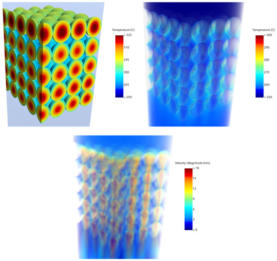
Figure 4.
Case 1, full power. Pebble temperature, fluid temperature, and fluid velocity fields for Strategy 3a (bridging 10%).
In general, the relative agreement of the other contact strategies decreased as the porosity error increased. The hydraulic QOIs were more sensitive than the thermal QOIs. The sensitivity of the contact strategy on the hydraulic QOIs was approximately 10 times greater than the observed differences when compared to the in the mesh convergence study. The sensitivity of the contact strategy on the thermal QOIs was approximately equal to the observed differences when compared to the in the mesh convergence study.
In Strategy 1, reducing the pebble volume, the Strategy 1a approach of a 0.1% diametral reduction performed the best: less than differences were observed for all the QOIs when compared to the baseline. On the other hand, Strategy 1c, with the error of porosity at , had the highest difference in QOIs; it significantly under-predicted the pressure drop and average velocity magnitude at and , respectively. For Strategy 2, this approach of increasing the pebble diameter was found to overestimate the pressure drop and average velocity magnitude. Only increasing the diameter by 0.1% yielded a small porosity error, but the simulations were not numerically stable unless a significantly finer mesh than required for the other strategies was used. A diametral increase yielded a porosity error of and large relative differences in pressure drop () and average velocity magnitude (). With respect to Strategy 3, changing the bridge diameter from to of the pebble diameter had a small impact. The largest differences were found to be less than . Strategy 4 underestimated the pressure drop and slightly underestimated the average fluid velocity, but it still yielded very similar pebble and fluid temperatures compared to the baseline.
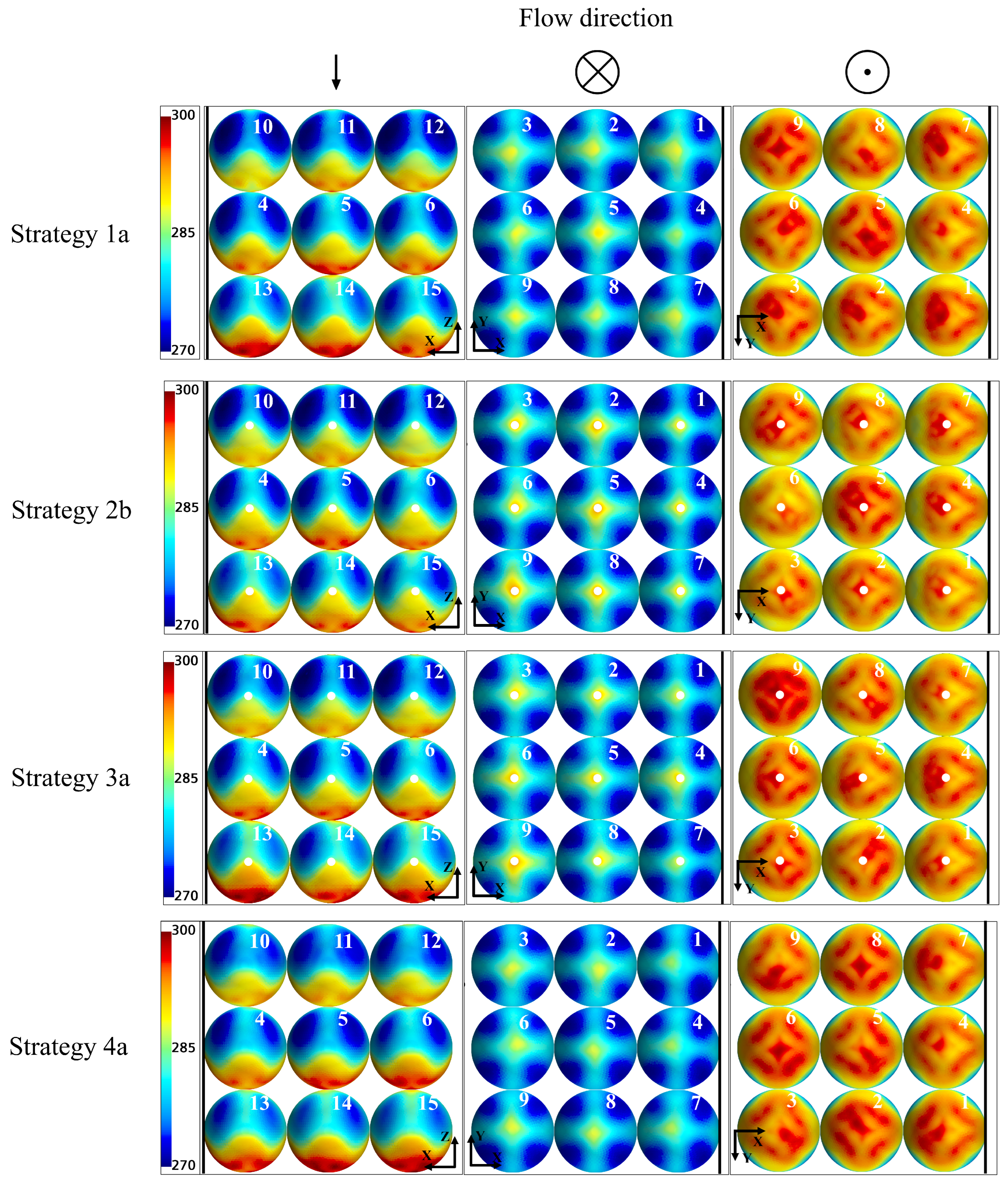
Figure 5 illustrates the surface temperature contours of the numbered pebbles along the views from a side view (-plane), a top view (-plane), and a bottom view (-plane) that were obtained using Strategies 1a, 2b, 3a, and 4a. Recall that Strategies 1 and 2 involve a simple modification of the pebble diameter, which is easy to implement for very large beds. On the other hand, Strategies 3 and 4 require considerable effort to produce the bridging between the contacting pebbles but were found to have lower porosity errors. Slight temperature differences are visible on the pebble downstream halves when viewed from the -plane bottom view.
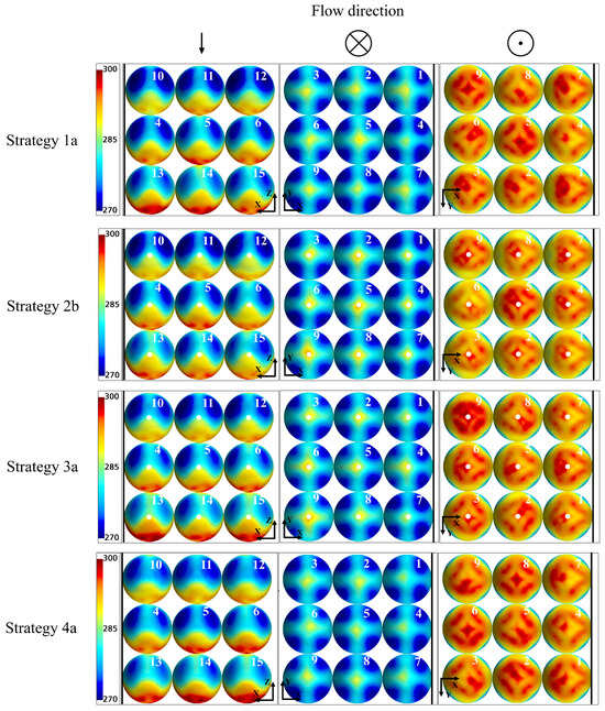
Figure 5.
Case 1, full power. Pebble surface temperatures (°C) for (row 1) Strategy 1a (diametral decrease of 0.1%) and (row 2) Strategy 2b (diametral increase of 0.5%), (row 3) Strategy 3a (bridge with dp), and (row 4) Strategy 4a (cap with 10% dp). From left to right: Pebble surface temperatures along the -plane side view, -plane top view, and -plane bottom view (see Figure 2).
Figure 6 depicts line integral convolution streamlines and velocity magnitudes along the - and -planes for Strategies 1a, 2b, 3a, and 4a. Among these contact strategies, the peaks of the velocity magnitude obtained from Strategies 1a and 3a appear the most similar for both the - and -planes. When comparing the velocity contours along the -plane (side view), the spatial positions of the velocity maxima were found to switch sides based on the contact strategy. For example, see pebble group 4-5-10-11. For the subchannels located in the vicinity of the reflector wall—that is, those that were created by pebbles 10-4-13 in the -plane and by pebbles 1-4-7 in -plane—all the tested pebble contact strategies revealed similar flow patterns. For instance, in each subchannel of pebbles 1-4-7, two pairs of counter-rotating vortices impinge on the pebble surfaces in each strategy.
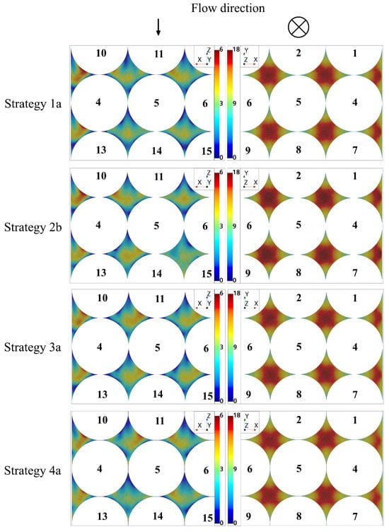
Figure 6.
Case 1, full power. Line integral convolution streamlines and velocity magnitudes for (row 1) Strategy 1a (diametral decrease of 0.1%) and (row 2) Strategy 2b (diametral increase of 0.5%), (row 3) Strategy 3a (bridge with 10% dp), and (row 4) Strategy 4a (cap with 10% dp) along the (left) -plane side view and (right) -plane top view.
3.2. Case 2: PLOFC
In Case 2, the four contact strategies were again investigated and roughly correspond to the PLOFC with a reactor trip event. This case was motivated by an objective to better understand the contact strategy under the separate effects of each heat transfer mode of conduction, convection, and radiation. For this case, the pebbles were assumed to have a temporally constant power density equal to 7% of the full-power density, which corresponds to approximately 20 s after the reactor trip [10].
Table 5 and Table 6 summarize the relative differences in the QOIs for each subcase. For Case 2a (conduction), the results are naturally divided into two groups based on whether or not the pebble bed was conductively connected (e.g., Strategies 2 and 3) or conductively isolated (e.g., Strategies 1 and 4). The conductively connected results had less than a 5% difference in the fuel and fluid temperatures, whereas the conductively isolated results differed significantly and diverged as the pebble volumes continued to decrease. The most different results were yielded by Strategies 1c and 4c, at approximately 25% and 22.9% differences, respectively, when predicting the maximum fuel temperature compared to the baseline results of Strategy 3a. As a consequence, the maximum fuel temperatures predicted by Strategies 1 and 4 were found to be considerably higher than those obtained from Strategies 2 and 3, where the pebble contacts are maintained. In addition, the fluid temperatures estimated using Strategies 1 and 4 were observed to be greater than those computed using Strategies 2 and 3; up to a 12.3% difference in was predicted using Strategy 1c.
Table 5.
Relative differences in QOIs computed from each pebble contact strategy for Cases 2a and 2b (%).
Table 6.
Relative differences in QOIs computed from various pebble contact strategies for Case 2c (%).
For Case 2b with conduction and radiation heat transfer modes, the temperature differences decreased significantly in both the solid and fluid regions. Strategy 1 slightly over-predicted the maximum fuel temperature within a 1.6% difference and fluid temperature with less than a 0.7% difference compared to the baseline results. The results of Strategy 2 were similar to the baseline, with differences of less than 0.7%. For Strategy 3, increasing the bridge size yielded greater differences in both the fuel and fluid temperatures compared to the baseline bridge 10% dp method. The temperatures computed using Strategy 4 varied from 0.4% to 0.8%.
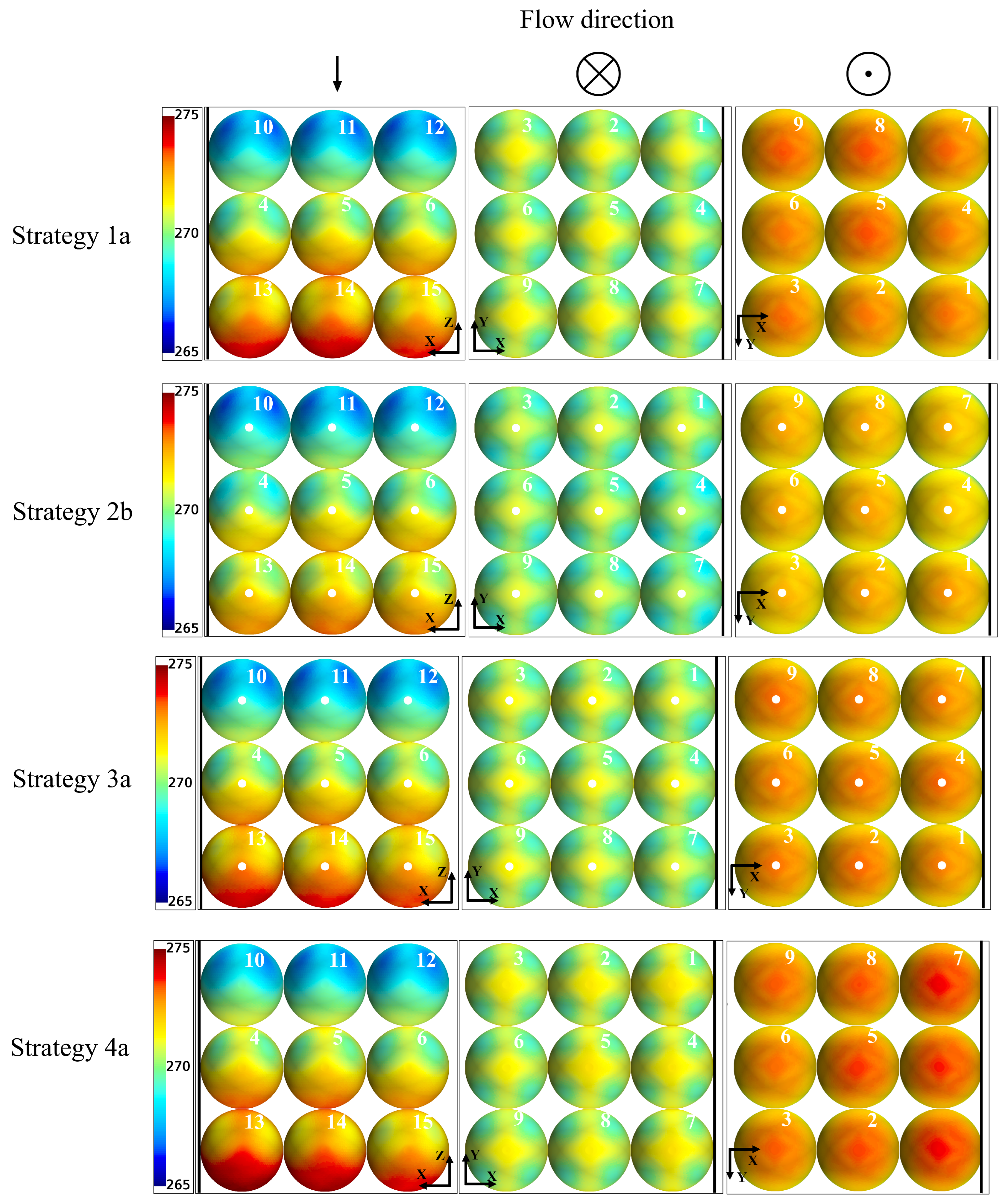
Figure 7 presents the Case 2c pebble surface temperatures along the views from the -plane (side view), -plane (top view), and -plane (bottom view) using Strategies 1a, 2b, 3a, and 4a. The pebble surface temperature contours from Strategy 2b were found to be lower than those from the baseline and other strategies. Table 6 highlights that the fluid velocity is the highest for Strategy 2, which explains the lower surface temperature. Nevertheless, the maximum and volume-averaged temperatures are nearly identical across the strategies.
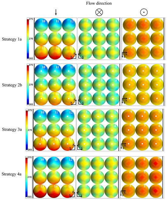
Figure 7.
Case 2c PLOFC pebble surface temperatures (°C) for (row 1) Strategy 1a (diametral decrease of ) and (row 2) Strategy 2b (diametral increase of 0.5%), (row 3) Strategy 3a (bridge with dp), and (row 4) Strategy 4a (cap with dp). From left to right: Pebble surface temperatures along the -plane side view, -plane top view, and -plane bottom view (see Figure 2).
Although the temperatures were not sensitive to the contact strategy, much larger variances were observed in the predictions of the maximum velocity—nearly 7.5% using Strategy 4c—and volume-averaged velocity, at 5.1% using Strategy 1c, within the bed. It can be concluded that any modification to the bed that increases or decreases the porosity, even slightly, results in larger differences in fluid velocity. This trend was also observed in the predictions of pressure drops from all the tested strategies. For instance, Strategy 1a (decrease 0.1%) with a 0.33% porosity error and Strategy 3a (decrease 1%) with a 3.26% porosity error yielded differences in pressure drop predictions of 1.2% and 19.1%, respectively, compared to the baseline. Similarly, varying the cap sizes from 10% (0.031% porosity error) to 20% (0.187% porosity error) caused the differences in the pressure drops to increase from 0.52% to 7.2%, respectively.
4. Discussion
This study numerically investigated the effects of various contact strategies on the flow and heat transfer behavior within a structured bed of 100 explicitly modeled pebbles. The pebbles were modeled as perfect spheres, and each had an inner spherical fuel region and an outer spherical shell fuel-free region. Four contact strategies and two thermal hydraulic conditions were considered. The strategies to avoid point-contact singularities included decreasing and increasing the pebble diameter, along with capping and bridging the pebble surfaces near the contact region. The two thermal hydraulic conditions were full-power operation (Case 1) and pressurized loss of forced cooling (Case 2).
The most desirable contact strategies are those that prioritize minimizing the porosity error as much as possible while providing a thermal connection to enable specifying an effective point-contact thermal resistance. Therefore, the recommended contact strategies and sizing selection are expected to hold for unstructured beds. Also, a study investigating externally heated unstructured beds reached similar conclusions as this effort with internally heated pebbles regarding the opportunity cost of each strategy and sizing recommendations [1].
Strategy 3a, bridging with a cylinder equal to 10% of the pebble diameter, was selected as the baseline strategy because it addressed the contact singularity while minimizing the geometric changes that affect the bed porosity.
For Case 1 (full power), the hydraulic behavior was sensitive to the various contact strategies, with a 30% difference in the predicted pressure drop (3% GCI) and a 4% difference for the volume-averaged velocity magnitude (0.1% GCI). The thermal behaviors within the pebbles and fluid were not sensitive to these changes as a difference of less than 0.5% (0.6% GCI) was observed across the strategies.
The strategy most similar to the baseline (Strategy 3a, bridge 10%) was Strategy 1a, with a pebble diametral reduction of 0.1%. However, the small fluid volumes created from the diametral reduction required an additional +12% of the volumetric elements to adequately resolve the RANS flow field.
A benefit of Strategy 3 is the simplification of specifying the interfacial thermal contact resistance between pebbles. This is because the bridges can be kept as separate regions during the model-building process. However, this bridge building is not trivial for large and unstructured beds. The contact patch definitions required for conformal interfaces become increasingly difficult for large-bed model building with bridging. These can be avoided with diametral reduction (Strategy 1) and chamfering (Strategy 4).
For Case 2 (PLOFC), large differences between the contact strategies were observed in the predicted pebble temperature when only considering thermal conduction. The difference in the maximum pebble temperatures for various strategies was 23% in Case 2a. When including radiation in Case 2b, the difference decreased to 2%. When adding 7% flow in Case 2c, the thermal differences decreased further to 0.3% for the various strategies. The hydraulic behavior’s sensitivity to the contact strategies in Case 2c was similar to the sensitivity observed in Case 1, where Strategy 1a was in close agreement with the baseline.
If the objective is to accurately predict the pressure drop and velocity distribution, Strategies 1a, 3, and 4a are recommended. Any larger diametral changes or large bridge sizes have too large of an impact on the bed porosity (>2% porosity error for global strategies). To accurately predict the temperature distribution within the fuel pebbles, any of the studied point-contact strategies are suitable when neglecting the thermal contact resistance. Strategy 3 simplifies the implementation of the interfacial thermal contact resistance between pebbles. Nevertheless, the geometry modifications of Strategy 1a can be achieved significantly faster for large and unstructured pebble beds.
Future efforts will focus on generating the experimental data of the temperature, pressure, and velocity fields for each contact strategy. For validation purposes, the data will then be compared with the numerical results of this paper.
Author Contributions
Conceptualization, N.G. and W.D.P.; methodology, N.G., T.N. and W.D.P.; software, N.G. and T.N.; formal analysis, N.G. and T.N.; investigation, N.G. and T.N.; resources, W.D.P.; writing—original draft preparation, N.G. and T.N.; writing—review and editing, N.G., T.N. and W.D.P.; visualization, N.G. and T.N.; supervision, W.D.P.; funding acquisition, W.D.P. All authors have read and agreed to the published version of the manuscript.
Funding
Funding for this work was provided by the US Department of Energy, Office of Nuclear Energy.
Institutional Review Board Statement
Not applicable.
Informed Consent Statement
Not applicable.
Data Availability Statement
The datasets presented in this article are not readily available because the data are part of an ongoing study. Requests to access the datasets should be directed to the corresponding author.
Acknowledgments
This manuscript has been authored by UT-Battelle LLC under contract no. DE-AC05-00OR22725 with the US Department of Energy (DOE). The US government retains and the publisher, by accepting the article for publication, acknowledges that the US government retains a nonexclusive, paid-up, irrevocable, worldwide license to publish or reproduce the published form of this manuscript or allow others to do so for US government purposes. DOE will provide public access to these results of federally sponsored research in accordance with the DOE Public Access Plan (http://energy.gov/downloads/doe-public-access-plan, accessed on 21 July 2024).
Conflicts of Interest
The authors declare no conflicts of interest. The funders had no role in the design of the study; in the collection, analyses, or interpretation of data; in the writing of the manuscript; or in the decision to publish the results.
Abbreviations
The following abbreviations are used in this manuscript:
| CFD | computational fluid dynamics. |
| DNS | direct numerical simulation. |
| FCC | face-centered cubic. |
| HALEU | high-assay low-enriched uranium. |
| LES | large-eddy simulation. |
| PIV | particle image velocimetry. |
| PLOFC | pressurized loss of forced cooling. |
| QOI | quantity of interest. |
| QOIs | quantities of interest. |
| RANS | Reynolds-averaged Navier–Stokes. |
| RMS | root mean square. |
| TRISO | tristructural isotropic. |
| URANS | Unsteady Reynolds-averaged Navier–Stokes. |
References
- Dixon, A.G.; Nijemeisland, M.; Stitt, E.H. Systematic mesh development for 3D CFD simulation of fixed beds: Contact points study. Comput. Chem. Eng. 2013, 48, 135–153. [Google Scholar] [CrossRef]
- Nijemeisland, M.; Dixon, A.G. CFD study of fluid flow and wall heat transfer in a fixed bed of spheres. AIChE J. 2004, 50, 906–921. [Google Scholar] [CrossRef]
- Shams, A.; Roelofs, F.; Komen, E.M.J.; Baglietto, E. Optimization of a Pebble Bed Configuration for Quasi-Direct Numerical Simulation. Nucl. Eng. Des. 2012, 242, 331–340. [Google Scholar] [CrossRef]
- Merzari, E.; Yuan, H.; Min, M.; Shaver, D.; Rahaman, R.; Shriwise, P.; Shriwise, P.; Talamo, A.; Lan, Y.; Gaston, D.; et al. Cardinal: A Lower Length-Scale Multiphysics Simulator for Pebble-Bed Reactors. Nucl. Technol. 2021, 27, 1118–1141. [Google Scholar] [CrossRef]
- Yildiz, M.A.; Botha, G.; Yuan, H.; Merzari, E.; Kurwitz, R.C.; Hassan, Y.A. Direct Numerical Simulation of the Flow through a Randomly Packed Pebble Bed. J. Fluids Eng. 2020, 142, 041405. [Google Scholar] [CrossRef]
- Dixon, A.G.; Walls, G.; Stanness, H.; Nijemeisland, M.; Stitt, E.H. Experimental validation of high Reynolds number CFD simulations of heat transfer in a pilot-scale fixed bed tube. Chem. Eng. J. 2012, 200, 344–356. [Google Scholar] [CrossRef]
- Guardo, A.; Coussirat, M.; Larrayoz, M.A.; Recasens, F.; Egusquiza, E. CFD flow and heat transfer in nonregular packings for fixed bed equipment design. Ind. Eng. Chem. Res. 2004, 43, 7049–7056. [Google Scholar] [CrossRef]
- Guardo, A.; Coussirat, M.; Recasens, F.; Larrayoz, M.; Escaler, X. CFD study on particle-to-fluid heat transfer in fixed bed reactors: Convective heat transfer at low and high pressure. Chem. Eng. Sci. 2006, 61, 4341–4353. [Google Scholar] [CrossRef]
- Agency, I.A.E. High Temperature Gas Cooled Reactor Fuels and Materials; International Atomic Energy Agency: Vienna, Austria, 2010. [Google Scholar]
- Boer, B.; Lathouwers, D.; Ding, M.; Kloosterman, J.L. Coupled Neutronics/Thermal Hydraulics Calculations for High Temperature Reactors with the DALTON-THERMIX Code System. In Proceedings of the of PHYSOR, Interlaken, Switzerland, 14–19 September 2008. [Google Scholar]
- Huning, A.J.; Chandrasekaran, S.; Garimella, S. A review of recent advances in HTGR CFD and thermal fluid analysis. Nucl. Eng. Des. 2021, 373, 111013. [Google Scholar] [CrossRef]
- Avramenko, A.; Dmitrenko, N.; Shevchuk, I.; Tyrinov, A.; Kovetskaya, M. Heat transfer and fluid flow of helium coolant in a model of the core zone of a pebble-bed nuclear reactor. Nucl. Eng. Des. 2021, 377, 111148. [Google Scholar] [CrossRef]
- Dixon, A.G.; Ertan Taskin, M.; Nijemeisland, M.; Stitt, E.H. Systematic mesh development for 3D CFD simulation of fixed beds: Single sphere study. Comput. Chem. Eng. 2011, 35, 1171–1185. [Google Scholar] [CrossRef]
- Shams, A.; Roelofs, F.; Komen, E.; Baglietto, E. Numerical simulation of nuclear pebble bed configurations. Nucl. Eng. Des. 2015, 290, 51–64. [Google Scholar] [CrossRef]
- Shams, A.; Roelofs, F.; Komen, E.; Baglietto, E. Numerical simulations of a pebble bed configuration using hybrid (RANS–LES) methods. Nucl. Eng. Des. 2013, 261, 201–211. [Google Scholar] [CrossRef]
- Shams, A.; Roelofs, F.; Komen, E.M.J.; Baglietto, E. Quasi-Direct Numerical Simulation of a Pebble Bed Configuration. Part I: Flow (Velocity) Field Analysis. Nucl. Eng. Des. 2013, 263, 473–489. [Google Scholar] [CrossRef]
- Hassan, Y.A.; Dominguez-Ontiveros, E. Flow visualization in a pebble bed reactor experiment using PIV and refractive index matching techniques. Nucl. Eng. Des. 2008, 238, 3080–3085. [Google Scholar] [CrossRef]
- Nguyen, T.; Muyshondt, R.; Hassan, Y.; Anand, N. Experimental investigation of cross flow mixing in a randomly packed bed and streamwise vortex characteristics using particle image velocimetry and proper orthogonal decomposition analysis. Phys. Fluids 2019, 31, 025101. [Google Scholar] [CrossRef]
- Lien, F.S. Low-Reynolds-number eddy-viscosity modelling based on non-linear stress-strain/vorticity relations. In Proceedings of the 3rd Symposium on Engineering Turbulence Modelling and Measurements, Heraklion-Crete, Greece, 27–29 May 1996; pp. 1–10. [Google Scholar]
- Wallin, S.; Johansson, A.V. An explicit algebraic Reynolds stress model for incompressible and compressible turbulent flows. J. Fluid Mech. 2000, 403, 89–132. [Google Scholar] [CrossRef]
- Hellsten, A. New advanced kw turbulence model for high-lift aerodynamics. AIAA J. 2005, 43, 1857–1869. [Google Scholar] [CrossRef]
- Shih, T.H.; Liou, W.W.; Shabbir, A.; Yang, Z.; Zhu, J. A new k-epsilon eddy viscosity model for high reynolds number turbulent flows. Comput. Fluids 1995, 24, 227–238. [Google Scholar] [CrossRef]
- Siemens. Simcenter STAR-CCM+ User Guide v. 16.02.009; Siemens: Munich, Germany, 2021. [Google Scholar]
- Reynolds, O. IV. On the dynamical theory of incompressible viscous fluids and the determination of the criterion. In Philosophical Transactions of the Royal Society of London.(a.); Royal Society Publishing: London, UK, 1895; pp. 123–164. [Google Scholar]
- Celik, I.B.; Ghia, U.; Roache, P.J.; Freitas, C.J. Procedure for Estimation and Reporting of Uncertainty Due to Discretization in CFD Applications. J. Fluids Eng. 2008, 130, 078001. [Google Scholar]


Disclaimer/Publisher’s Note: The statements, opinions and data contained in all publications are solely those of the individual author(s) and contributor(s) and not of MDPI and/or the editor(s). MDPI and/or the editor(s) disclaim responsibility for any injury to people or property resulting from any ideas, methods, instructions or products referred to in the content. |
© 2024 by the authors. Licensee MDPI, Basel, Switzerland. This article is an open access article distributed under the terms and conditions of the Creative Commons Attribution (CC BY) license (https://creativecommons.org/licenses/by/4.0/).